Weakest-Link Scaling and Extreme Events in Finite-Sized Systems

Abstract

Weakest-link scaling is used in the reliability analysis of complex systems. It is characterized by the extensivity of the hazard function instead of the entropy. The Weibull distribution is the archetypical example of weakest-link scaling, and it describes variables such as the fracture strength of brittle materials, maximal annual rainfall, wind speed and earthquake return times. We investigate two new distributions that exhibit weakest-link scaling, i.e., a Weibull generalization known as the κ-Weibull and a modified gamma probability function that we propose herein. We show that in contrast with the Weibull and the modified gamma, the hazard function of the κ-Weibull is non-extensive, which is a signature of inter-dependence between the links. We also investigate the impact of heterogeneous links, modeled by means of a stochastic Weibull scale parameter, on the observed probability distribution.

1. Introduction

In statistical mechanics, the velocities of non-interacting particles are viewed as random variables that follow the Maxwell–Boltzmann distribution. Quantities of interest are often macroscopic (system) properties, such as the energy or the entropy, that involve averages over many particles. Evaluating these properties involves calculating averages over suitable probability distributions. Randomness is also a factor in the analysis of macroscopic variables. Environmental time series, energy and mineral reserves and earthquakes are just a few examples of phenomena that exhibit stochastic fluctuations. In addition, the lifetimes (times to failure) of various natural and engineered materials and devices are also random variables. In contrast with statistical mechanics, there is a strong interest not only in average quantities, but also in the extreme values of such distributions [1]. The classical extreme value theory studies the probability distributions of extreme events [2,3]. The Fisher–Tippet–Gnedenko theorem shows that the distribution of suitably-scaled transformations of the maxima or minima of a collection of independent and identically distributed (i.i.d.) variables follows the generalized extreme value (GEV) distributions, which include the Gumbel, Weibull and Fréchet distributions. The type of GEV obtained depends on the tail behavior of the probability distribution for the i.i.d. random variables. Extensions that involve stochastic scalings have been recently proposed in [4].

We investigate systems that obey the weakest-link scaling (WLS) principle. In the WLS framework, the system response (e.g., material strength) is controlled by the weakest link (unit), which implies a marked deviation from statistical independence. The Weibull model [3] is the archetypical probability distribution for WLS systems and is widely used in reliability modeling [5]. It finds application as a model of the fracture strength of brittle and quasi-brittle technological materials [6,7] and geologic media [8], waiting times between earthquakes [9–15], wind speed [16] and annual hydrological maxima [17]. We study the impact of the randomness (heterogeneity) of the Weibull link parameters on the system survival function by introducing doubly-stochastic representations analogous to superstatistics [18]. We also investigate weakest-link scaling with non-exponential link survival functions. In this context, we introduce a modified gamma distribution, and we provide theoretical arguments for the κ-Weibull distribution, which exhibits power-law tails in finite-sized systems.

1.1. Mathematical Preliminaries

We will use the capital letter X to denote a random variable (e.g., tensile strength, wind speed, earthquake return time, maximum annual rainfall or river discharge) and the lowercase x to denote values of the random variable, where x ∈ [0, ∞). We will assume that the random variable represents the property of interest for a particular spatial or temporal window (support), the size of which we will denote by ℓ. The probability density function (pdf) will be denoted by f_ℓ(x). It is customary to use f_X(x) to denote the pdf of X when more than one random variable is involved. In this case, however, there is no risk of confusion, and thus, we replace X with the support scale, which is relevant in our analysis. The integral of the pdf, i.e., the cumulative distribution function (cdf), will be denoted by:

$$F_{\ell }(x)={\displaystyle {\int }_{-\infty }^x\mathrm{d}{x}^{\prime }{f}_{\ell }(x^{\prime }).}$$

Another useful probability function, which is mostly used in reliability analysis, is the survival function or complementary cumulative distribution function, defined by:

$$R_{\ell }(x)=1-F_{\ell }(x).$$

(1)

The survival function R_ℓ(x) gives the probability that the system has not “failed” when the variable X has reached the level x. The survival function is equal to one for x = x_min and tends to zero for x → ∞. A characteristic property of the survival function is that its integral equals the expectation of X, i.e.,

$$\mathbb{E}[X]={\displaystyle {\int }_0^{\infty }\mathrm{d}{x}^{\prime }{R}_{\ell }(x^{\prime }).}$$

(2)

The above is based on dR_ℓ(x)/dx = −f_ℓ(x), which follows from (1) and integration by parts.

• In the case of fracture strength, R_ℓ(x) is the probability that the system has not failed if the external load takes values that do not exceed x.
• In the case of earthquake return times, the survival function is the probability that there are no successive earthquakes separated by a time interval less than or equal to x.
• In the case of annual rainfall maxima, R_ℓ(x) gives the probability that the maximum rainfall over the support area for the duration of one year does not exceed the value x.

Finally, the hazard rate or hazard function h_ℓ(x) is the conditional probability that the system will fail at time x* > x within the infinitesimal time window x < x* ≤ x + δx, given that the system has not failed during the interval [0, x]. Let A denote the event that the system has not failed at x and B the event that the system fails at x < x* ≤ x + δx. Then, h_ℓ(x) = Prob(B|A) = Prob(B ∩ A)/Prob(A), which leads to the following:

$$h_{\ell }(x)=\frac{\mathrm{Prob}(x<x^{\ast }\le x+\delta x)}{R_{\ell }(x)\delta x}=\frac{f_{\ell }(x)}{R_{\ell }(x)}.$$

(3)

The asymptotic dependence of the hazard rate is a matter of interest. For example, in the case of earthquakes, it is often desired to estimate the probability of the time until the next big earthquake. If the particular hazard rate tends to infinity as x → ∞, the probability that an earthquake will occur increases with the time elapsed since the last earthquake [19]. In contrast, a decreasing or constant hazard rate indicates that the probability of a new occurrence is reduced or remains constant, respectively, as time elapses, and no event takes place.

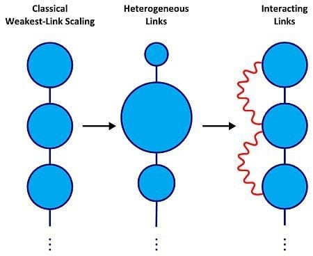
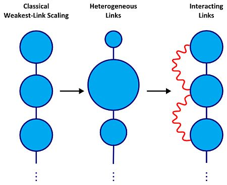
2. Weakest-Link Scaling Theory

The weakest-link scaling (WLS) theory has been developed to model the strength of disordered systems based on the strengths of “critical elements” or links [20]. In WLS, the entire system fails if the link with the lowest mechanical strength breaks, hence the term “weakest-link”. The foundations of weakest-link theory are found in the studies of Gumbel [2] and Weibull [3] on the statistics of extremes. The concept of links is straightforward in simple systems, e.g., one-dimensional chains. In higher dimensions, the links correspond to critical subsystems, the failure of which causes an avalanche, leading to the failure of the entire system.

Weakest-link scaling is used in statistical physics to investigate size effects in the strength of heterogeneous materials [6,21–23]. In reliability modeling, a weakest-link system is known as a series system [24]. The same scaling ideas, however, can be used in other systems, as well. For example, in the case of maximum annual rainfall, the scale links could correspond to single days and the system scale to an entire year. Then, if “one link fails,” i.e., if the rainfall on a specific day exceeds the specified threshold x, then the “entire system fails,” i.e., the maximum annual daily rainfall also exceeds the threshold.

Let us consider a system with support ℓ_N consisting of N links with support ℓ₀. The WLS premise is then expressed as follows:

$$R_{{\ell }_N}(x)={\displaystyle \prod _{i=1}^N{R}_{i;{\ell }_0}(x),}$$

(4)

where $R_{i;{\ell }_0}(x)$ refers to the survival function of the i-th link. If we assume that all of the links have a common survival function, then (4) can be expressed as:

$$R_{{\ell }_N}(x)={\left[R_{{\ell }_0}(x)\right]}^N.$$

(5)

The above leads to an additive relation for the logarithms of the survival function, i.e.,

$$\ln R_{{\ell }_N}(x)=N\ln R_{{\ell }_0}(x).$$

(6)

Now, if we take into account that:

$$\frac{\mathrm{d}\ln R_{{\ell }_N}(x)}{\mathrm{d}x}=\frac{1}{R_{{\ell }_N}(x)}\frac{\mathrm{d}{R}_{{\ell }_N}(x)}{\mathrm{d}x}=-\frac{f_{{\ell }_N}(x)}{R_{{\ell }_N}(x)}=-h_{{\ell }_N}(x),$$

(7)

it follows from (6) that the WLS hazard function satisfies the additive property:

$$h_{{\ell }_N}(x)=N{h}_{{\ell }_0}(x).$$

(8)

For a system of N independent and identically distributed random variables, it holds that:

$$f_{{\ell }_N}(x)={\displaystyle \prod _{i=1}^N{f}_{{\ell }_0}(x).}$$

Equation (5) implies that under WLS conditions, the link independence does not hold, since:

$$f_{{\ell }_N}(x)=-\frac{\mathrm{d}{R}_{{\ell }_N}(x)}{\mathrm{d}x}=N{\left[R_{{\ell }_0}(x)\right]}^{N-1}{f}_{{\ell }_0}(x),$$

(9)

which is markedly different from the link independence condition.

To compare general WLS distribution functions with the Weibull, we use the double logarithm of the reciprocal survival probability,

$$\mathrm{\Phi }\left(x;{\ell }_N\right):=\ln \left[\ln \left(1/R_{{\ell }_N}(x)\right)\right].$$

(10)

If $F_{{\ell }_N}(x)$ follows the Weibull dependence, then $\mathrm{\Phi }(x;{\ell }_N)=m\ln \frac{x}{x_s}$.

For a general WLS distribution, we obtain the following relation based on (5):

$$\mathrm{\Phi }\left(x;{\ell }_N\right)=\ln N+\ln \left[-\ln R{\ell }_0(x)\right].$$

(11)

The above scaling relation in combination with (10), replacing ℓ_N in the latter with ℓ₀, implies the following scaling property:

$$\mathrm{\Phi }(x;{\ell }_N)=\ln N+\mathrm{\Phi }\left(x;{\ell }_0\right).$$

(12)

2.1. Systems Composed of Interacting Links

Above, we assumed an identical survival function for all of the links, a condition that is plausible in a mean-field framework. Herein, we consider systems in which the link properties vary. This is an interesting possibility, which can lead to new probability models for reliability engineering. In general, if R_i;ℓ0(x) = Prob(Λ_i) is the probability that the i-th link survives, the system’s survival probability under WLS conditions is given by:

$$R_{{\ell }_N}(x)=\mathrm{Prob}\left({\mathrm{\Lambda }}_1\cap {\mathrm{\Lambda }}_2\dots \cap {\mathrm{\Lambda }}_N\right).$$

Using the law of joint probability it follows that:

$$R_{{\ell }_N}(x)=\mathrm{Prob}({\mathrm{\Lambda }}_1)\mathrm{Prob}({\mathrm{\Lambda }}_2|{\mathrm{\Lambda }}_1)\dots \mathrm{Prob}({\mathrm{\Lambda }}_{{\ell }_N}|{\mathrm{\Lambda }}_1,\dots ,{\mathrm{\Lambda }}_{N-}{}_1).$$

The conditional probability Prob(Λ₂|Λ₁) may in general depend on the state of Λ₁ and the degree of interaction between the two links. This agrees with the observation of complex interaction patterns in geological fault systems, if the links are identified with single faults or fault groups [25]. One possibility for expressing this dependence is by means of the following ansatz:

$$\mathrm{Prob}\left({\mathrm{\Lambda }}_2|{\mathrm{\Lambda }}_1\right)=R_{{\ell }_0}({\lambda }_{1}x),$$

where λ₁ > 0 is a scaling factor. Since $R_{{\ell }_0}(·)$ is a decreasing function, λ₁ > 1 implies that the conditional survival probability of Λ₂ is reduced compared to the probability $R_{{\ell }_0}(x)$.

More generally, for an N-link system, the survival function of the link Λ_i can be expressed as:

$$\mathrm{Prob}\left({\mathrm{\Lambda }}_{{\ell }_i}|{\mathrm{\Lambda }}_1,\dots ,{\mathrm{\Lambda }}_{i-}{}_1\right)=R_{{\ell }_0}\left({\lambda }_{i-}{}_{1}x\right),i=2,\dots N.$$

In light of the above, the system survival function is given by the following equation:

$$R_{{\ell }_N}(x,\overrightarrow{\lambda })=R_{{\ell }_0}(x){\displaystyle \prod _{i=2}^N{R}_{{\ell }_0}({\lambda }_{i-1}x)},$$

(13)

which is determined by the coefficient vector $\overrightarrow{\lambda }={\left({\lambda }_1,{\lambda }_2,\dots ,{\lambda }_{N-1}\right)}^T$. The above system survival function is given by a product rule in agreement with the survival function (4) of the homogeneous-link system. In addition, all terms of the product involve the same function $R_{{\ell }_0}(·)$, albeit the argument of the latter is modified by the respective coefficients λ_i, i = 1, …, N − 1. Hence, (13) maintains the product rule and the same functional form of the link survival function, which are central features of WLS, but it also captures interactions between the links via the coefficients $\overrightarrow{\lambda }$. We illustrate the behavior of the system survival function for a fictitious two-link system in Figure 1, where $R_{{\ell }_2}(x,\lambda )$ is compared with $R_{{\ell }_2}(x,1)={[R_{{\ell }_0}(x)]}^2$: the former is the survival function of the correlated system, whereas the latter is the standard WLS survival function. For the Weibull survival function, λ effectively renormalizes the scale parameter x_s to $x_s^{\prime }={[2/(1+{\lambda }^m)]}^{1/m}{x}_s$. Hence, the ansatz (13) essentially accounts for the correlations by renormalizing a parameter of the “free distribution”, which is an idea with deep roots in statistical physics. Figure 1 demonstrates that values λ > 1 (λ < 1) lead to lower (higher) survival probability for the same x than the uniform-link WLS function.

The proposed system survival function (13) is quite general, since it allows for different functional forms of the link survival function. In (13), it is possible to consider correlated random variables λ_i as coefficients. In this case, the random variable X becomes doubly stochastic and is described by superstatistics [18,26]. We expect that the variability of link parameters is a plausible scenario in heterogeneous physical or engineered systems. For example, a theoretical framework has been proposed that links the statistics of earthquake recurrence times to fracture strength in the Earth’s crust [15,27]. Since the crust is a heterogeneous material decorated with flaws (faults) of widely varying sizes and orientations, it is reasonable to expect that the fracture strength parameters exhibit local random fluctuations in addition to systematic changes with depth [25].

2.2. Hazard Function for Links with Variable Parameters

There is a distinct possibility that links have different statistical properties, even in the case of engineered materials. Thus, a link parameter θ can become a random variable with pdf g(θ). In light of the additivity property (4), the hazard rate of the system is given by the following sum:

$$h_{{\ell }_N}(x)={\displaystyle \sum _{i=1}^N{h}_{i;{\ell }_0}(x;\theta ).}$$

(14)

We can define the average hazard function over the links:

$${\overline{h}}_{{\ell }_0}(x)=\frac{1}{N}{\displaystyle \sum _{i=1}^N{h}_{i;{\ell }_0}(x;\theta ),}$$

so that $h_{{\ell }_N}(x)=N{\overline{h}}_{{\ell }_0}(x)$. If θ follows the pdf g(θ), and the support of θ is the finite interval [θ_min, θ_max], we can define an effective link hazard rate $h_{{\ell }_0}^{*}(x)$ by:

$$h_{{\ell }_0}^{*}(x)={\displaystyle {\int }_{{\theta }_{min}}^{{\theta }_{max}}d\theta h_{{\ell }_0}(x,\theta )g(\theta )}.$$

(15)

If $h_{{\ell }_0}(x,\theta )$ and g(θ) are continuous functions of θ, the requirements of the mean value theorem are fulfilled; thus, there exists a θ* ∈ [θ_min, θ_max], such that:

$$h_{{\ell }_0}^{*}(x)=h_{{\ell }_0}(x|{\theta }^{*}){\displaystyle {\int }_{{\theta }_{min}}^{{\theta }_{max}}d\theta g(\theta )=h_{{\ell }_0}(x|{\theta }^{*})}.$$

(16)

Equation (16) states that the effective link hazard rate maintains the original functional form and that the impact of random θ can be described by means of an “effective parameter” θ*, provided that the conditions of the mean value theorem are upheld.

If ergodic conditions are satisfied so that the events on the links sufficiently sample the space of probable states, one can assume that ${\overline{h}}_{{\ell }_0}(x)=h_{{\ell }_0}^{*}(x)$. The observed survival function then is $R_{{\ell }_0}(x)=R_{{\ell }_0}(x|{\theta }^{*})$, and:

$$\mathrm{\Phi }(x;{\ell }_0)=\ln [-\ln (R_{{\ell }_0}(x|{\theta }^{*}))],$$

(17)

which implies that:

$$\mathrm{\Phi }(x;{\ell }_0)=\mathrm{\Phi }(x;{\ell }_0|{\theta }^{*}).$$

(18)

2.3. Observed Distributions for Non-ergodic Conditions

In the case of natural phenomena, however, the available sample is often finite, and the ergodic condition may not be justifiable. For example, an earthquake catalog for a particular area covers only a small portion of the area’s geological history. This means that the full ensemble, involving both the distribution of the scale parameters and the distribution of x values for fixed parameter values, is not adequately sampled during the observation process. If g(θ) has a narrow mode (e.g., Weibull with m > 1), the estimated pdf ĝ(θ) will have a peak in the interval [θ_min, θ_max] near the mode of g(θ). For disperse parameter distributions (e.g., Weibull with m ≤ 1), ĝ(θ) may exhibit more complicated behavior due to insufficient sampling.

In order to illustrate the effect of the sample size and the link parameter’s variability on the observed link probability distribution, we conduct a numerical experiment. We simulate a random variable X that represents individual links, assuming that X follows the Weibull distribution $f_{{\ell }_0}(x;m,x_s)$ with a fixed shape parameter m and uniformly distributed scale parameter x_s. The distribution of x_s is g(x_s) = (x_s;max − x_s;min)⁻¹ if x_s ∈ [x_s;min, x_s;max] and g(x_s) = 0 otherwise. We generate a large set containing n_total = 10⁶ random numbers drawn from Weibull distributions with different values of x_s. The latter correspond to different links drawn from the uniform distribution g(x_s). We define the mixing ratio as the number of sampled links over the number of samples per link, i.e.,

$$\rho =\frac{N}{n_s},N=\#\text{number of links},n_s=\#\text{samples per link}$$

The ratio ρ determines the mixing of random values from distributions with different scale parameters. Small values of ρ denote that a small number of links are sampled compared to the samples taken from each link, whereas high values of ρ denote the opposite.

In order to investigate different mixing scenarios, we consider two values of ρ equal to 0.1 and 10⁻⁴. The lower limit x_s;min of the scale parameter distribution is set to one, whereas the width δ = x_s;max − x_s;min of the uniform distribution is set to δ = 1 and 100. From the initial set of n_total random numbers, we randomly select n = 10³ and 10⁵ samples, for each of the four scenarios obtained by the different combinations of ρ and δ. The different values of n allow investigating the sample size effect. For each sample, we calculate the maximum likelihood estimates of the optimal-fit Weibull parameters, which are listed in

Table 1. Estimates of Weibull distribution parameters for the simulated data of Figure 2.

			m = 0.7		m = 2.5
N	δ	ρ	${\widehat{x}}_s$	$\widehat{m}$	${\widehat{x}}_s$	$\widehat{m}$
103	1	10−4	1.39	0.688	1.42	2.14
		10−1	1.55	0.694	1.54	2.25
	100	10−4	45.6	0.592	51.8	1.23
		10−1	43.6	0.634	49.6	1.38
105	1	10−4	1.40	0.689	1.42	2.19
		10−1	1.50	0.691	1.52	2.23
	100	10−4	57.0	0.679	59.3	1.94
		10−1	42.9	0.611	48.4	1.30

. For m = 0.7, the sample-based estimates of the Weibull modulus are close to the true value, especially in the case of the narrower distribution of the scale parameter. For m = 2.5, the estimates of the Weibull modulus are close to the true value only for the narrow scale parameter distribution.

We also show the estimated $\widehat{\mathrm{\Phi }}(x;\ell )$ derived from the empirical (sample-based) cumulative distribution function in Figure 2. For reference purposes, if the data follow the Weibull distribution, $\widehat{\mathrm{\Phi }}(x;\ell )$ is a straight line with slope $\widehat{m}$ and intercept $\widehat{m}\ln {\widehat{x}}_s$. As shown in Figure 2(c), for m < 1 and large n, the Weibull distribution is obtained. For smaller n (Figure 2(a)), deviations from the Weibull emerge. For m > 1 and small n, the data cannot be described with a Weibull distribution (Figure 2(b)). For a larger sample size (Figure 2(d)), $\widehat{\mathrm{\Phi }}(x;\ell )$ demonstrates Weibull tails with different slopes. Overall, for m = 0.7 (in general, for m < 1), the distribution of sampled values maintains, albeit approximately, the Weibull characteristic shape and the original modulus. For m > 1, the Weibull scaling is maintained only for a narrow scale parameter distribution.

3. Exponential and Non-Exponential Link Survival Functions

Whereas the Weibull distribution has proven quite successful in the analysis of extreme value data, in certain cases, deviations from the Weibull scaling have been noticed in the tails of empirical distributions [27,28]. As shown above, such deviations could occur due to fluctuations of the link hazard rate parameters. Below, we investigate a different possibility, which is based on non-exponential link survival functions with deterministic parameters. Ideally, such functions should be obtained from microscopic theories that describe the dynamics of the relevant physical processes inside the links. Nevertheless, the definition of links and their respective probability functions is not always possible in terms of such detailed analysis [6,28]. Hence, for practical purposes, it is useful to consider phenomenological definitions of the survival function.

3.1. Weibull Link Ansatz

In his original paper, Weibull assumed that $R_{{\ell }_0}(x)={\mathrm{e}}^{-\varphi }{}^{(x)}$, where φ(x) ≥ 0 is a monotonically increasing function [3]. In particular, he proposed that ϕ(x) = (x/x_s)^m, where x_s is the scale parameter and m is the shape parameter or Weibull modulus. More generally, the exponential dependence $R_{{\ell }_n}(x)={\mathrm{e}}^{-\varphi }{}^{(x)}$, implies the self-similarity relation:

$$R_{{\ell }_N}(x)=R_{{\ell }_{N/2}}(x)R_{{\ell }_{N/2}}(x)=\dots ={\left[R_{{\ell }_0}(x)\right]}^{2^{\mathrm{m}}},N=2^m.$$

(19)

This self-similarity property implies that the survival function for any cluster comprising several links has the same functional form, except for a trivial size scaling, as the single-link survival function.

The Weibull distribution can also be derived without invoking the exponential dependence of the link survival function. This approach is based on the additivity of the logarithmic survival functions, i.e.,

$$\ln R_{{\ell }_N}(x)={\displaystyle \sum _{i=1}^N\ln R_{{\ell }_0}(x)}={\displaystyle \sum _{i=1}^N\ln \left[1-F_{{\ell }_0}(x)\right]}.$$

Since the system’s failure is caused by the weakest link, we can assume that for $N\gg 1$, this occurs at x, such that $F_{{\ell }_0}(x)\ll 1$. Thus, we can use the approximation:

$$\ln R_{{\ell }_N}(x)\approx -N{F}_{{\ell }_0}(x)\Rightarrow R_{{\ell }_N}(x)\approx {\mathrm{e}}^{-N}{}^{F_{{\ell }_0}(x)}.$$

Next, one assumes that $F_{{\ell }_0}(x)\approx {(x/x_s)}^m$, x < x_c, where x_c is a threshold above which the algebraic dependence of $F_{{\ell }_0}(x)$ ceases. This argument leads to the Weibull expression; however, it does not clarify the tail behavior of the distribution function for $x\gg x_c$.

Based on the self-similarity relation (19) and the pioneering works of Daniels and Smith [29,30] that use a Gaussian strength distribution for the links, Curtin showed that the strength distribution of heterogeneous materials tends asymptotically to the Weibull form and that the system’s strength parameters depend on both the system and the link sizes [21].

3.2. Non-Exponential Link Ansatz

An acceptable link survival function should satisfy the following properties: (i) it should take real values in the interval [0, 1]; (ii) it should be a monotonically decreasing function of x. Let us introduce the following simple functional form:

$$R_{{\ell }_0}(x)=\sqrt{1+{\varphi }^2(x)}-\varphi (x),$$

(20)

which gives admissible survival functions if ϕ(x) satisfies (i) ϕ(0) = 0, (ii) lim_x→∞ ϕ(x) → ∞ and (iii) ϕ(x) is a monotonically increasing function of x. Condition (iii) is necessary to ensure that $\mathrm{d}{R}_{{\ell }_0}(x)/\mathrm{d}x\le 0$, because the latter is given by:

$$\frac{\mathrm{d}{R}_{{\ell }_0}(x)}{\mathrm{d}x}=\frac{\mathrm{d}\varphi (x)}{\mathrm{d}x}\left[\frac{\varphi (x)}{\sqrt{1+{\varphi }^2(x)}}-1\right].$$

The second term in the product on the right-hand side of the above is negative, and thus, $\mathrm{d}{R}_{{\ell }_0}(x)/\mathrm{d}x\le 0$ only if dϕ(x)/dx ≥ 0.

In light of (7), one can then show that the hazard function is given by:

$$h(x)=\frac{\mathrm{d}\varphi (x)}{\mathrm{d}x}\frac{1}{\sqrt{1+{\varphi }^2(x)}}.$$

(21)

Hence, for x ≫ 1, i.e., ϕ(x) →∞, it holds that h(x) ≈ d ln ϕ(x)/dx.

The main appeal of (20) is its simplicity. On the other hand, the condition (19) requires solving the following set of nonlinear equations:

$$\sqrt{1+{\varphi }_{{\ell }_{N/2}}^2(x)}-{\varphi }_{{\ell }_{N/2}}(x)={\left[\sqrt{1+{\varphi }^2(x)}-\varphi (x)\right]}^{N/2},\text{for all}N=2^{2m},m=1,2,\dots ,$$

which is satisfied by:

$${\varphi }_{{\ell }_{N/2}}(x)=\frac{1-{\left[\sqrt{1+{\varphi }^2(x)}-\varphi (x)\right]}^N}{2{\left[\sqrt{1+{\varphi }^2(x)}-\varphi (x)\right]}^{N/2}}.$$

The above, however, does not lead to a self-similar expression for ${\varphi }_{{\ell }_{N/2}}(x)$.

In the following sections, we investigate certain probability distributions for systems with a finite number of links that are based on non-exponential link survival functions.

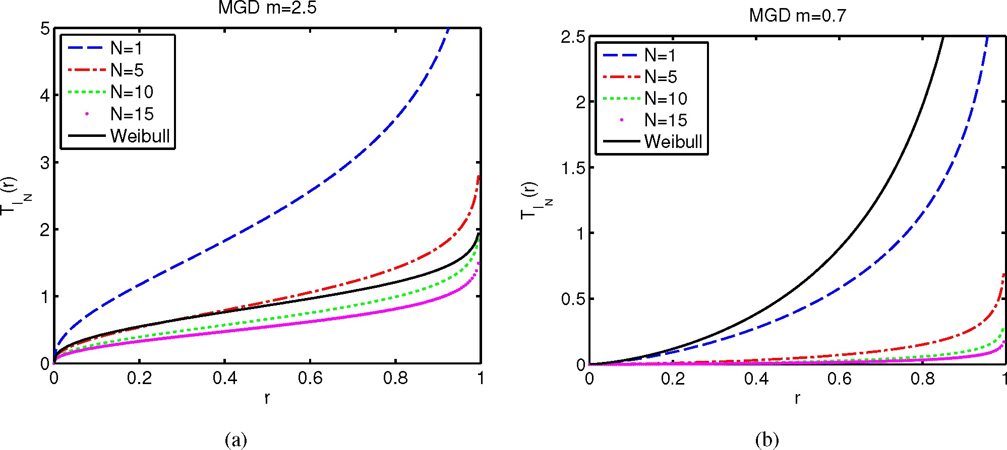
4. Finite-Size System with Gamma Link Distribution

4.1. The Gamma Distribution

First, we consider a slight modification of the exponential link survival function, which is based on the gamma distribution.

$$F_{{\ell }_0}(x)=F\gamma (x):=\frac{1}{\mathrm{\Gamma }(m)}\gamma (x/x_s,m),$$

(22)

where x_s and m are respectively the scale and shape parameters, γ(z, m) is the lower incomplete gamma function defined by means of the integral:

$$\gamma (z,m)={\displaystyle {\int }_0^z\mathrm{d}u{u}^{m-1}{e}^{-u}},$$

(23)

and Γ(m) is the gamma function that is obtained from γ(z, m) at the asymptotic limit, Γ(m) = lim_z→∞ γ(z, m). The pdf of the gamma distribution is given by:

$$f_{\gamma }(x)=\frac{x^{m-}{}^1{\mathrm{e}}^{-x/x_s}}{\mathrm{\Gamma }(m)x_s^m}.$$

(24)

The hazard rate of the gamma distribution is respectively given by:

$$h_{{\ell }_0}(x)=\frac{e^{-x/x_s}}{\gamma (x/x_s,m)x_s}{\left(\frac{x}{x_s}\right)}^{m-1}.$$

(25)

4.2. The Modified Gamma Distribution

We use the WLS scaling relation (5) and a gamma link probability function to define the modified gamma distribution, which applies to the entire system as follows:

$$F_{{\ell }_N}(x)=1-{[1-F_{\gamma }(x)]}^N=1-{[R_{{\ell }_0}(x)]}^N.$$

(26)

The quantile function (inverse survival function) of the modified gamma distribution is:

$$T_{{\ell }_N}(r)=x_s{\gamma }^{-1}[\mathrm{\Gamma }(m)(1-r^{1/N}),m],$$

(27)

where γ⁻¹(·) is the inverse of the lower incomplete gamma function. The quantile function of the modified gamma distribution is plotted in Figure 3. The median of the modified gamma distribution is $x_{\mathrm{med}}=T_{{\ell }_N}(1/2,m)$, i.e.,

$$x_{\mathrm{med}}=x_s{\gamma }^{-1}\left[\mathrm{\Gamma }(m)\left(1-\frac{1}{\sqrt[N]{2}}\right),m\right].$$

(28)

Based on (5) and assuming uniform link parameters, Equation (9) leads to the following modified gamma pdf for the N-link system:

$$f_{{\ell }_N}(x)=N\frac{e^{-x/x_s}}{\mathrm{\Gamma }(m)x_s}{\left(\frac{x}{x_s}\right)}^{m-1}{\left[1-\frac{\gamma (x/x_s,m)}{\mathrm{\Gamma }(m)}\right]}^{N-1}.$$

(29)

Equation (29) can also be expressed as:

$$f_{{\ell }_N}(x)=f_{\gamma }(x)g_{{\ell }_N}(x),$$

where f_γ(x) is given by (24) and $g_{{\ell }_N}(x)$ is a modulation function given by:

$$g_{{\ell }_N}(x)=N{[1-F_{\gamma }(x)]}^{N-1}=N{[R_{{\ell }_0}(x)]}^{N-1}.$$

(30)

The hazard rate of the modified gamma distribution is given according to (8) by:

$$h_{{\ell }_N}(x)=\frac{f_{{\ell }_N}(x)}{R_{{\ell }_N}(x)}=N{h}_{{\ell }_0}(x),$$

(31)

4.3. Motivation and Properties

The gamma distribution is used in reliability engineering to model extreme events, such as the lifetime of devices, the intensity of rainfall and earthquake return times [1]. The gamma distribution is also known in statistical physics as the stretched exponential distribution for m < 1, whereas it defaults to the exponential distribution for m = 1.

The modified gamma survival function is constructed assuming an WLS system that comprises N links that have an identical link failure probability that follows the gamma cdf. The modulation function $g_{{\ell }_N}(x)$ given by (30) takes values between N (at x = 0) and zero (at x → ∞). For m > 1 and increasing N, $g_{{\ell }_N}(x)$ shifts the mode of the pdf to lower values and reduces the width of the peak, as shown in Figure 4(a). Increasing N also suppresses the right tail of the pdf. The gamma distribution is obtained for N = 1, as it is easily verified from (29). For m < 1, as N increases, the $g_{{\ell }_N}(x)$ increases the values of $f_{{\ell }_N}(x)$ as x → 0 and reduces the right tail, as shown in Figure 4(b). For m < 1, $f_{{\ell }_N}(x)\to \infty$ as x → 0.

The gamma hazard rate is plotted in Figure 5; it is an increasing function for x < x_s, whereas at $x\gg 1$, it is dominated by the exponential dependence, which leads to an asymptotically constant hazard function. In contrast, the Weibull distribution for m > 1 has a hazard rate that increases with x [13,19].

In Figure 6 we plot the cdf and Φ(x; ℓ_N) of the modified gamma distribution for m = 0.7, m = 2.5 and for different values of N. We compare these functions to the respective functions for the Weibull distribution. For m > 1, the Φ(x; ℓ_N) curves are straight lines on the Weibull plot for ln(x/x_s) ≤ a_c, where a_c ≈ −1, but become concave as ln(x/x_s) increases further. This means that the right tail of the modified gamma distribution is heavier than the respective Weibull tail. In contrast, for m < 1, the Φ(x; ℓ_N) curve becomes convex upwards for ln(x/x_s) > a_c, and the right tail of the modified gamma distribution is lighter than the respective Weibull tail. The Φ(x; ℓ_N) curves of the modified gamma distribution for different N with fixed m collapse onto a single curve by parallel shifting, in agreement with the scaling relation (12).

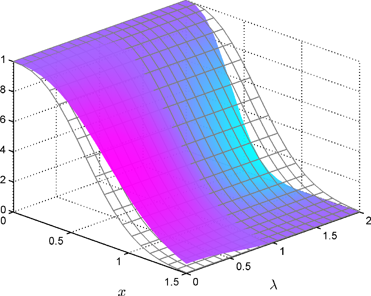
5. Finite-Sized System with κ-Weibull Distribution

5.1. The κ-exponential and κ-logarithm Functions

The definition of the κ-exponential function for κ ≥ 0 is given by [31–35]:

$${\exp }_{\kappa }(z)={\left(\sqrt{1+z^2{\kappa }^2}+z\kappa \right)}^{1/\kappa }.$$

(32)

The κ-exponential tends asymptotically to the standard exponential at the limits z → 0 or κ → 0, i.e.,

$${\exp }_{\kappa }(z)\underset{z\to 0}{\sim }\exp (z),$$

(33a)

$${\exp }_{\kappa }(z)\underset{\kappa \to 0}{\sim }\exp (z).$$

(33b)

The inverse function of the κ-exponential is the κ-logarithm, which is defined by:

$${\ln }_{\kappa }(z)=\frac{z^{\kappa }-z^{-\kappa }}{2\kappa }.$$

(34)

5.2. The κ-Weibull Function

If κ = 1/N, where N is the number of links in a system, we can define a system survival function based on:

$$R_{{\ell }_N}(x)={\exp }_{\kappa }\left[-{\left(\frac{x}{x_s}\right)}^m\right].$$

(35)

The κ-Weibull admits explicit expressions for the cdf, the survival function and the pdf, which are given respectively by the following expressions:

$$F_{\kappa }(x)=1-{\exp }_{\kappa }(-{[x/x_s]}^m),$$

(36)

$$R_{\kappa }(x)={\exp }_{\kappa }(-{[x/x_s]}^m),$$

(37)

$$f_{\kappa }(x)=\frac{m}{x_s}{\left(\frac{x}{x_s}\right)}^{m-1}\frac{{\exp }_{\kappa }(-{[x/xs]}^m)}{\sqrt{1+{\kappa }^2{(x/x_s)}^{2m}}}.$$

(38)

The κ-Weibull hazard function is obtained from (31) using (37) and (38) as follows:

$$h_{\kappa }(x)=\frac{m}{x_s}\frac{{(x/x_s)}^{m-1}}{\sqrt{1+{\kappa }^2{(x/x_s)}^{2m}}}.$$

(39)

The κ-Weibull quantile function is defined by means of the survival function as follows:

$$T_{\kappa }(R_{\kappa })=\frac{1}{x_s}{\left[{\ln }_{\kappa }\left(\frac{1}{R_{\kappa }}\right)\right]}^{1/m}.$$

(40)

5.3. Motivation and Properties

The κ-Weibull is motivated by the non-exponential link ansatz discussed in Section 3.2. In particular, we assume that ϕ(x) is the following monotonically increasing function with link-size dependence:

$$\varphi (x)=\frac{1}{N}{(x/x_s)}^m.$$

Then, the link survival function is given according to (20) by the function:

$$R_{{\ell }_0}(x)=\sqrt{1+\frac{1}{N^2}{\left(\frac{x}{x_s}\right)}^{2m}}-\frac{1}{N}{\left(\frac{x}{x_s}\right)}^m.$$

The κ-Weibull system survival function (35) is then obtained from the above link survival function and the WLS principle (5).

Based on the properties of the κ-exponential, the survival function (35) corresponds to an extension of the Weibull survival function. The term κ-Weibull is due to the presence of the κ-exponential. This distribution has been used in economics to model the distribution of income [32,34] and in statistical physics as a model of earthquake recurrence times [27]. Other potential applications include the fracture strength of quasi-brittle materials, which exhibit deviations from Weibull scaling [7,28], and reliability models that involve the Pareto distribution.

The κ-exponential function can describe heavy-tailed processes, because for κ > 0, it decays asymptotically as a power-law function, i.e.,

$${\exp }_{\kappa }(z)\underset{z\to \pm \infty }{\sim }{|2\kappa z|}^{\pm 1/\kappa }.$$

(41)

The κ-Weibull pdf also exhibits a power-law tail, which is inherited by the κ-exponential and is relevant in applications where such heavy tails are observed. In addition, if we define the κ-Weibull plot by means of the function Φ′_κ(x) = ln ln_κ(1/R_κ(x)), it follows that Φ′_κ(x) = m ln (x/x_s). Hence, Φ′_κ(x) is independent of κ and regains the logarithmic scaling of the double logarithm of the inverse survival function. This means that the κ-Weibull plot, in which Φ′_κ(x) is plotted instead of Φ_κ(x), can be used to visually detect the κ-Weibull scaling.

Plots of the κ-Weibull pdf for x_s = 1 and two values of m (m < 1 and m > 1) are shown in Figure 7. The plots also include the Weibull pdf (κ = 0) for comparison. For both m, lower N lead to a heavier right tail. For m = 2.5 the mode of the pdf moves to the right as N increases (for m = 0.7 the mode is at zero independently of N, since the distribution is zero-modal for m ≤ 1) [34]. To the right of the mode, higher N correspond, at first, to higher pdf values. This is reversed at a crossover point beyond which the lower-N pdfs exhibit slower power-law decay, i.e., lim_x→∞ f_κ(x) ∝ x^−α, where α = 1 + m/κ [34]. The crossover point occurs at ≈ 1.5x_s for m = 2.5, whereas for m = 0.7 at ≈ 5 x_s.

6. Conclusions

We investigated the statistical implications of the principle of weakest-link scaling. This type of scaling is used to model the probability distributions of extreme events, including the failure strength of various heterogeneous materials, wind speed, earthquake recurrence times and hydrological maxima. We have focused on various statistical mechanisms leading to deviations from the Weibull distribution, which is commonly used in weakest-link scaling systems. Our motivation stems from empirical distributions that deviate from the Weibull in physical systems expected to follow weakest-link scaling, e.g., [7,15,27,28,36]. Our results include a modified gamma distribution, the κ-Weibull distribution and weakest-link scaling distributions with non-homogeneous links that have random (possibly correlated) parameters. The distributions proposed above modify the tail behavior in comparison with the classical Weibull dependence. We thus believe that they are of interest to both statistical physicists and reliability or systems engineers.

The modified gamma distribution, which we introduce herein, is derived by applying weakest-link scaling to systems with a finite number of links. The modified gamma distribution has a heavier tail than the respective Weibull for m > 1 and a lighter tail for m < 1. The κ-Weibull distribution is also shown to follow from weakest-link scaling. A notable property of the κ-Weibull distribution is its ability to exhibit a power-law tail, whereas the modified gamma distribution is dominated by exponential decay at large values. The power-law dependence of the κ-Weibull is derived from the interaction between the system and the links, expressed in terms of a finite-valued scaling factor N in the link survival function. For N → ∞, the κ-Weibull tends to the Weibull model, and the power-law decay at x ≫ 1 is replaced by the exponential Weibull dependence. We have argued in [27] that the κ-Weibull distribution can be observed in the case of earthquake recurrence times if the monitored area comprises a finite number of faults. We have also linked the number of effective units in this system to the inverse of κ. This type of behavior can also be observed if the system under study does not include all of the units (e.g., faults) of an interdependent system. In this case, events that are outside the boundaries of the observed system are not taken into account, thus leading to longer recurrence times, which generate the power-law tail. The heavy tail of the κ-Weibull may also find applications in biology, e.g., in modeling the inter-spike interval distributions of cortical neurons, which is known to follow a power law [37].

We have also proposed a different approach for inserting correlations in weakest-link scaling systems by means of a variable scaling factor in the link survival function. If this factor is random (but possibly correlated between links), the observed random variable X is described by an appropriate superstatistics formulation. In the case of Weibull link scaling, we have shown that if the scale parameter is uniformly distributed and uncorrelated across links, the observable probability distribution is controlled by three factors: the width of the scale parameter distribution, the Weibull modulus and the mixing ratio, which determines the balance between the number of links and the values contributed by each link to the observed sample. In the limit of a very large sample, it is also shown that the system’s survival function regains the Weibull form, albeit with a renormalized scale, provided that the distribution of the scale parameter has a compact support. In further research, we will investigate the impact of correlations between link distribution parameters on the observed system survival function, as well as applications of this formalism to environmental extreme events that exhibit weakest-link scaling.

Another extreme value distribution that fits within the weak-scaling formalism is the Gumbel distribution [38]. The Gumbel distribution is of the general form F (x) = exp(− exp(−x)) and belongs to the family of generalized extreme value distributions. The Gumbel is characterized by a different mathematical expression and size scaling than the Weibull distribution. There is both theoretical and experimental evidence (e.g., in the fracture of brittle ceramics) that in certain cases, the Gumbel is a more suitable asymptotic form than the Weibull [22,38]. One may therefore wonder if the same arguments that led to the κ-Weibull distribution also apply to the Gumbel distribution. At this point, however, we lack insight into how this construction should be implemented. Hence, we will leave this as an open subject for future research.

References

1. Sornette, D. Critical Phenomena in Natural Sciences; Springer: Berlin, Germany, 2004. [Google Scholar]
2. Gumbel, E.J. Les valeurs extrêmes des distributions statistiques. Annales de l’Institut Henri Poincaré 1935, 5, 115–158. [Google Scholar]
3. Weibull, W. A statistical distribution function of wide applicability. J. Appl. Mech. 1951, 18, 293–297. [Google Scholar]
4. Eliazar, I.; Klafter, J. Randomized central limit theorems: A unified theory. Phys. Rev. E 2010, 82, 021122. [Google Scholar]
5. Barlow, R.E.; Proschan, F. Mathmatical Theory of Reliability; SIAM: Philadelphia, PA, USA, 1996. [Google Scholar]
6. Hristopulos, D.T.; Uesaka, T. Structural disorder effects on the tensile strength distribution of heterogeneous brittle materials with emphasis on fiber networks. Phys. Rev. B 2004, 70, 064108. [Google Scholar]
7. Pang, S.D.; Bažant, Z.; Le, J.L. Statistics of strength of ceramics: Finite weakest-link model and necessity of zero threshold. Int. J. Fract. 2008, 154, 131–145. [Google Scholar]
8. Amaral, P.M.; Fernandes, J.C.; Rosa, L.G. Weibull statistical analysis of granite bending strength. Rock Mech. Rock Eng. 2008, 41, 917–928. [Google Scholar]
9. Hagiwara, Y. Probability of earthquake occurrence as obtained from a Weibull distribution analysis of crustal strain. Tectonophysics 1974, 23, 313–318. [Google Scholar]
10. Rikitake, T. Recurrence of great earthquakes at subduction zones. Tectonophysics 1976, 35, 335–362. [Google Scholar]
11. Rikitake, T. Assessment of earthquake hazard in the Tokyo area, Japan. Tectonophysics 1991, 199, 121–131. [Google Scholar]
12. Holliday, J.R.; Rundle, J.B.; Turcotte, D.L.; Klein, W.; Tiampo, K.F.; Donnellan, A. Space-Time Clustering and Correlations of Major Earthquakes. Phys. Rev. Lett. 2006, 97, 238501. [Google Scholar]
13. Abaimov, S.G.; Turcotte, D.L.; Rundle, J.B. Recurrence-time and frequency-slip statistics of slip events on the creeping section of the San Andreas fault in central California. Geophys. J. Int. 2007, 170, 1289–1299. [Google Scholar]
14. Abaimov, S.G.; Turcotte, D.; Shcherbakov, R.; Rundle, J.B.; Yakovlev, G.; Goltz, C.; Newman, W.I. Earthquakes: Recurrence and Interoccurrence Times. Pure Appl. Geophys. 2008, 165, 777–795. [Google Scholar]
15. Hristopulos, D.T.; Mouslopoulou, V. Strength statistics and the distribution of earthquake interevent times. Physica A 2013, 392, 485–496. [Google Scholar]
16. Conradsen, K.; Nielsen, L.; Prahm, L. Review of Weibull statistics for estimation of wind speed distributions. J. Clim. Appl. Meteorol. 1984, 23, 1173–1183. [Google Scholar]
17. Van den Brink, H.; Können, G. The statistical distribution of meteorological outliers. Geophys. Res. Lett. 2008, 35. [Google Scholar] [CrossRef]
18. Beck, C.; Cohen, E. Superstatistics. Physica A 2003, 322, 267–275. [Google Scholar]
19. Sornette, D.; Knopoff, L. The paradox of the expected time until the next earthquake. Bull. Seismol. Soc. Am. 1997, 87, 789–798. [Google Scholar]
20. Chakrabarti, B.K.; Benguigui, L.G. Statistical Physics of Fracture and Breakdown in Disordered Systems; Clarendon Press: Oxford, UK, 1997. [Google Scholar]
21. Curtin, W.A. Size Scaling of Strength in Heterogeneous Materials. Phys. Rev. Lett. 1998, 80, 1445–1448. [Google Scholar]
22. Alava, M.J.; Phani, K.V.V.N.; Zapperi, S. Statistical models of fracture. Adv. Phys. 2006, 55, 349–476. [Google Scholar]
23. Alava, M.J.; Phani, K.V.V.N.; Zapperi, S. Size effects in statistical fracture. J. Phys. D 2009, 42, 214012. [Google Scholar]
24. Ditlevsen, O.D.; Madsen, H.O. Structural Reliability Methods; Wiley: Chichester, UK and New York, NY, USA, 1996. [Google Scholar]
25. Mouslopoulou, V.; Hristopulos, D.T. Patterns of tectonic fault interactions captured through geostatistical analysis of microearthquakes. J. Geophys. Res. Solid Earth. 2011, 116. [Google Scholar] [CrossRef]
26. Cohen, E. Superstatistics. Physica D 2004, 193, 35–52. [Google Scholar]
27. Hristopulos, D.T.; Petrakis, M.; Kaniadakis, G. Finite-size Effects on Return Interval Distributions for Weakest-link-scaling Systems. Phys. Rev. E 2014, 89, 052142. [Google Scholar]
28. Bažant, Z.P.; Le, J.L.; Bažant, M.Z. Scaling of strength and lifetime probability distributions of quasi-brittle structures based on atomistic fracture mechanics. Proc. Natl. Acad. Sci. USA. 2009, 1061, 11484–11489. [Google Scholar]
29. Daniels, H.E. The statistical theory of the strength of bundles of threads. Proc. R. Soc. A 1945, 183, 405–435. [Google Scholar]
30. Smith, R.L.; Phoenix, S.L. Asymptotic distributions for the failure of fibrous materials under series-parallel structure and equal load sharing. J. Appl. Mech. 1981, 48, 75–82. [Google Scholar]
31. Kaniadakis, G. Statistical mechanics in the context of special relativity II. Phys. Rev. E 2005, 72, 036108. [Google Scholar]
32. Clementi, F.; Di Matteo, T.; Gallegati, M.; Kaniadakis, G. The κ-generalized distribution: A new descriptive model for the size distribution of incomes. Physica 2008, 387, 3201–3208. [Google Scholar]
33. Kaniadakis, G. Maximum Entropy Principle and power-law tailed distributions. Eur. Phys. J. B 2009, 70, 3–13. [Google Scholar]
34. Clementi, F.; Gallegati, M.; Kaniadakis, G. A κ-generalized statistical mechanics approach to income analysis, 2009; arXiv:0902.0075.
35. Kaniadakis, G. Theoretical Foundations and Mathematical Formalism of the Power-Law Tailed Statistical Distributions. Entropy 2013, 15, 3983–4010. [Google Scholar]
36. Bažant, Z.P.; Pang, S.D. Activation energy based extreme value statistics and size effect in brittle and quasi-brittle fracture. J. Mech. Phys. Solids. 2007, 55, 91–131. [Google Scholar]
37. Tsubo, Y.; Isomura, Y.; Fukai, T. Power-Law Inter-Spike Interval Distributions Infer a Conditional Maximization of Entropy in Cortical Neurons. PLoS Comput. Biol. 2012, 8, e1002461. [Google Scholar]
38. Manzato, C.; Shekhawat, A.; Nukala, P.K.V.V.; Alava, M.J.; Sethna, J.P.; Zapperi, S. Fracture Strength of Disordered Media: Universality, Interactions, and Tail Asymptotics. Phys. Rev. Lett. 2012, 108, 065504. [Google Scholar]
Figure 1. Survival function R 2 ( x , λ ) for a system comprising two links that follow the Weibull survival function R 0 ( x ) with xs = 1 and m = 2.5. Continuous surface: R 2 ( x , λ ) for different values of λ. Mesh: R 2 ( x , 1 ).
Entropy 17 01103f1
Figure 2. Sample estimates Φ ^ ( x ; ) of data sets with sizes n = 103 (top) and n = 105 (bottom). The samples are randomly drawn from a total of ntotal = 106 simulated values generated from Weibull distributions with fixed m = 0.7 (left column) and m = 2.5 (right column). The xs are uniformly distributed in the interval [1, 1 + δ] with δ = 1, 100. The mixing ratio that determines the number of xs values (links) over the number of random values per link is ρ = 0.1, 10−4.
Entropy 17 01103f2
Figure 3. Quantile function for the modified gamma distribution (27) with m = 2.5 (a) and m = 0.7 (b) for different link sizes N (shown with different line types).
Entropy 17 01103f3
Figure 4. Modified gamma distribution pdf f N ( x ) with m = 2.5 (a) and m = 0.7 (b) for different link sizes N (shown with different line types).
Entropy 17 01103f4
Figure 5. Hazard rate h 0 ( x ) of the gamma probability distribution for m = 2.5 (a) and m = 0.7 (b).
Entropy 17 01103f5
Figure 6. Cumulative distribution function F N ( x ) (left) and associated Φ(x; N) (right) for the modified gamma distribution with m = 2.5 (top) and m = 0.7 (bottom) and different values of N (shown by different line types), as well as the respective Weibull functions with the corresponding Weibull modulus.
Entropy 17 01103f6
Figure 7. Semi-logarithmic plots of κ-Weibull pdfs for xs = 1, different values of N (shown by different line types), and Weibull modulus equal to (a) m = 2.5 (b) m = 0.7.
Entropy 17 01103f7