Kappa and q Indices: Dependence on the Degrees of Freedom

Abstract

The kappa distributions, or their equivalent, the q-exponential distributions, are the natural generalization of the classical Boltzmann-Maxwell distributions, applied to the study of the particle populations in collisionless space plasmas. A huge step in the development of the theory of kappa distributions and their applications in space plasma physics has been achieved with the discovery that the observed kappa distributions are connected with the solid statistical background of non-extensive statistical mechanics. Now that the statistical framework has been identified, it is straightforward to improve our understanding of the nature of the kappa index (or the entropic q-index) that governs these distributions. One critical topic is the dependence of the kappa index on the degrees of freedom. In this paper, we first show how this specific dependence is naturally emerged, using the formalism of the N-particle kappa distribution of velocities. Then, the result is extended in the presence of potential energies. It is shown that the kappa index is simply related to the kinetic and potential degrees of freedom. In addition, it is shown that various problems of non-extensive statistical mechanics, such as (i) the correlation dependence on the total number of particles; and (ii) the normalization divergence for finite kappa indices, are resolved considering the kappa index dependence on the degrees of freedom.

1. Introduction

Thermal equilibrium is a special stationary state. It is the state where any flow of heat (e.g., thermal conduction, thermal radiation) is in balance. Systems at thermal equilibrium have one very special statistical feature: not only are their particle velocities described by stationary distribution functions, but also, any of these functions is some Maxwellian distribution.

Numerous independent developments in space plasma physics have revealed the peculiar statistical behavior of this category of systems: particle populations in space plasmas reside in stationary states out of thermal equilibrium. The classical Maxwell distributions are extremely rare in space plasmas. On the contrary, the vast majority of space plasmas reside out of thermal equilibrium, and are described by the kappa distributions (e.g., see [1–4] and references therein).

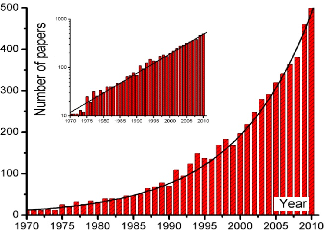
The kappa distributions were empirical statistical models of the velocities of particle populations in space plasmas. A breakthrough in the field of space physics came with the connection of the observed kappa distributions with the solid theoretical framework of “Non-Extensive Statistical Mechanics” [1], in contrast to the Maxwell distributions, which are connected with the classical Boltzmann-Gibbs Statistical Mechanics. Since then, the kappa distributions have become increasingly widespread across space physics with the number of relevant publications following, remarkably, an exponential growth rate (Figure 1).

Space plasmas are essentially collisionless particle systems out of thermal equilibrium, which are typically described by kappa distributions (single types or combinations thereof). Single types of these distributions are usually sufficient to model the space plasma populations (e.g., see [5–10]); however, more complicated models of kappa distribution superpositions have been employed to describe rare features (e.g., anisotropy) [11,12]. A kappa distribution is primarily formulated to describe a Hamiltonian [13], i.e., the sum of the particle’s kinetic and potential energies. However, the potential energy of a particle is small compared to its kinetic energy and can often be ignored; then, the system’s statistical description is reduced to the kappa distribution of the particle velocities.

Numerous analyses have established the theory of kappa distributions and provided a plethora of different applications in space plasmas. In particular, kappa distributions described numerous space plasma populations in: (i) the inner heliosphere, including, solar wind (e.g., [2,11,14–21]), solar corona (e.g., [22–25]), solar energetic particles (e.g., [26,27]), corotating interaction regions (e.g., [28]), solar flares (e.g., [6,15]); (ii) the planetary magnetospheres, including, the general magnetosphere (e.g., [29]), magnetosheath (e.g., [30–32]), magnetotail (e.g., [33]), ring current (e.g., [34]), plasma sheet (e.g., [35–37]), magnetospheric substorms (e.g., [38]), Jovian/Saturnian/Uranian/Neptunian magnetospheres [39–41]), magnetospheres of planetary moons (e.g., Io, Enceladus) (e.g., [42,43]); (iii) the outer heliosphere and inner heliosheath (e.g., [3–10,44–50]); (iv) beyond the heliosphere, including HII regions (e.g., [51]), planetary nebula (e.g., [51,52]), supernova magnetospheres (e.g., [53]); and other general plasma related fields, such as linear and nonlinear plasma waves (e.g., [21,54]), solitary waves (e.g., [55]), and dusty plasmas (e.g., [56]). (See also [1–4] and references therein.)

The purpose of this paper is to show and study the dependence on the degrees of freedom, of the non-equilibrium measure that governs kappa distributions, the kappa index, which is also related to the entropic q-index of non-extensive statistical mechanics. Section 2 briefly presents the connection of kappa distributions with non-extensive statistical mechanics. Section 3 focuses on the dependence of the standard kappa index on the degrees of freedom. A new kappa index is developed that is invariant under variation of the degrees of freedom. This is shown using the N-particle kappa distribution of velocities, without a potential energy. Section 4 shows the formulations of kappa distributions with or without potential energy using the developed invariant kappa index. Section 5 shows the invariant kappa index is developed in the general case, using the N-particle kappa distribution of positions and velocities, in the presence of potential energy. In Section 6, we discuss the inconsistencies caused by the dependence of the kappa index on the degrees of freedom, and how these are resolved by the invariant kappa index. Finally, Section 7 summarizes the conclusions.

2. Connection of Kappa Distributions with Non-Extensive Statistical Mechanics

The Maxwell distribution is the canonical distribution in the classical framework of Boltzmann-Gibbs (BG) statistical mechanics that applies only at thermal equilibrium. Maximizing the BG entropy under the constraints of the canonical ensemble, the Boltzmann’s exponential distribution of energy is derived. This exponential distribution of energy gives the Maxwellian distribution of velocities in the absence of any potential energy, where the total energy is reduced to the kinetic energy.

Similarly, the kappa distribution is the canonical distribution in the generalized framework of non-extensive statistical mechanics that applies both in and out of thermal equilibrium. Maximizing the Tsallis entropy, under the constraints of the canonical ensemble (that includes the mean kinetic energy using the “escort” probability distribution), a q-deformed exponential distribution of energy is derived. This becomes the q-Maxwellian distribution of velocities after the substitution of the kinetic energy, and as it has been shown, it is equivalent to the kappa distribution, under the transformation between the entropic index q (used in non-extensive statistical mechanics) and the kappa index κ (used in space and plasma physics):

$$\mathrm{\kappa }=1/(q-1)\iff q=1+1/\mathrm{\kappa }$$

(1)

The connection with non-extensive statistical mechanics is based on three fundamental physical notions and formulations: (i) Tsallis entropy [57–59]; (ii) escort probability distribution [58–60]; and (iii) physical temperature [1–5,59,61–63].

The entropy is a functional of $p(\overrightarrow{u})$, which is the “ordinary” probability distribution in the velocity space:

$$S[p(\overrightarrow{u})]=\frac{1}{q-1}\cdot \left\{1-{\displaystyle {\int }_{-\infty }^{+\infty }{\left[p(\overrightarrow{u})\cdot {\sigma }_u{}^f\right]}^{q}d\mathrm{\Omega }}\right\}$$

(2)

where σ_u is the smallest speed-scale parameter characteristic of the system, so that the number of microstates in the f-dimensional phase space is $d\mathrm{\Omega }\equiv {\sigma }_u{}^{-f}d{u}_{1}d{u}_2\dots d{u}_f$ [3,6].

The entropy is maximized under the constraint of normalization:

$$1={\displaystyle {\int }_{-\infty }^{+\infty }\left[p(\overrightarrow{u})\cdot {\sigma }_u{}^f\right]d\mathrm{\Omega }}$$

(3)

and the constraint of the mean kinetic energy $<\mathrm{\epsilon }>$:

$$0={\displaystyle {\int }_{-\infty }^{+\infty }{\left[p(\overrightarrow{u})\cdot {\sigma }_u{}^f\right]}^q\cdot [\mathrm{\epsilon }(\overrightarrow{u})-<\mathrm{\epsilon }>]d\mathrm{\Omega }}$$

(4)

The derived ordinary probability distribution of energy (for a given q-index) is:

$$p(\mathrm{\epsilon })~{\left[1+(q-1)\cdot \frac{\mathrm{\epsilon }(\overrightarrow{u})-\langle \mathrm{\epsilon }\rangle }{k_{B}T}\right]}_{}^{\frac{1}{1-q}}$$

(5)

The corresponding “escort” distribution that constitutes the canonical distribution (in terms of energy) is $P(\mathrm{\epsilon })~p{(\mathrm{\epsilon })}^q$, i.e.:

$$P(\mathrm{\epsilon })~{\left[1+(q-1)\cdot \frac{\mathrm{\epsilon }(\overrightarrow{u})-\langle \mathrm{\epsilon }\rangle }{k_{B}T}\right]}_{}^{\frac{q}{1-q}}$$

(6)

where $\mathrm{\epsilon }(\overrightarrow{u})=(1/2)m{(\overrightarrow{u}-<\overrightarrow{u}>)}^2$ is the particle kinetic energy, and the mean kinetic energy defines the temperature [1–5,59,61–63] according to:

$$\langle \mathrm{\epsilon }\rangle =\frac{1}{2}m\cdot \langle {(\overrightarrow{u}-<\overrightarrow{u}>)}^2\rangle =\frac{d}{2}{k}_{\mathrm{B}}T\text{or}\langle {(\overrightarrow{u}-<\overrightarrow{u}>)}^2\rangle =\frac{d}{2}\cdot {\theta }^2$$

(7)

The average particle velocity represents the bulk speed of the flow of particles, ${\overrightarrow{u}}_b\equiv <\overrightarrow{u}>$. The quantity $\theta \equiv \sqrt{2k_{\mathrm{B}}T/m}$ is the thermal speed of particle of mass m, that is, the particle temperature T expressed in speed units; both the particle $\overrightarrow{u}$ and bulk ${\overrightarrow{u}}_b$ velocities are in an inertial reference frame.

Furthermore, using the notion of kappa index, $\mathrm{\kappa }=1/(q-1)$ [1], the q-Maxwell distribution is transformed to its equivalent, the so-called kappa distribution:

$$P(\mathrm{\epsilon })~{\left[1+\frac{1}{\mathrm{\kappa }}\cdot \frac{\mathrm{\epsilon }-\langle \mathrm{\epsilon }\rangle }{k_{B}T}\right]}_{}^{-\mathrm{\kappa }-1}~{\left[1+\frac{1}{\mathrm{\kappa }-\frac{f}{2}}\cdot \frac{\mathrm{\epsilon }}{k_{B}T}\right]}_{}^{-\mathrm{\kappa }-1}$$

(8)

In terms of the velocity, the escort distribution $P(\overrightarrow{u})$ generalizes the classical Maxwell distribution, and is called q-Maxwellian distribution:

$$P(\overrightarrow{u})~{\left[1+\frac{q-1}{1-\frac{f}{2}(q-1)}\cdot \frac{{(\overrightarrow{u}-{\overrightarrow{u}}_b)}^2}{{\theta }^2}\right]}_{}^{\frac{q}{1-q}}~{\left[1+\frac{1}{\mathrm{\kappa }-\frac{f}{2}}\cdot \frac{{(\overrightarrow{u}-{\overrightarrow{u}}_b)}^2}{{\theta }^2}\right]}_{}^{-\mathrm{\kappa }-1}$$

(9)

Note that the physical temperature, T or $\theta \equiv \sqrt{2k_{\mathrm{B}}T/m}$, represents the actual temperature of the system. Its thermodynamic definition is given by $T\equiv {(\partial S/\partial U)}^{-1}\cdot [1-\frac{1}{\mathrm{\kappa }}\cdot S/k_{{\rm B}}]$ (U is the internal energy–that equals to the kinetic energy in the absence of a potential energy) [61] showed that only this type of relation is consistent with the Zero-th law of Thermodynamics. Livadiotis and McComas [1,20] showed the equality between the kinetic and thermodynamic temperature definitions, and thus produced a well-defined temperature for systems out of thermal equilibrium that are describable by kappa distributions.

3. The Invariant Kappa Index

3.1. The N-particle Kappa Distributions

The N-particle phase-space kappa distribution is given by:

$$P({\overrightarrow{r}}_1,{\overrightarrow{r}}_2,\dots ,{\overrightarrow{r}}_N;{\overrightarrow{u}}_1,{\overrightarrow{u}}_2,\dots ,{\overrightarrow{u}}_N)~{\left[1+\frac{1}{\mathrm{\kappa }}\cdot \frac{H({\overrightarrow{r}}_1,{\overrightarrow{r}}_2,\dots ,{\overrightarrow{r}}_N;{\overrightarrow{u}}_1,{\overrightarrow{u}}_2,\dots ,{\overrightarrow{u}}_N)-\langle H\rangle }{k_{B}T}\right]}^{-\mathrm{\kappa }-1}$$

(10)

where $H({\overrightarrow{r}}_1,{\overrightarrow{r}}_2,\dots ,{\overrightarrow{r}}_N;{\overrightarrow{u}}_1,{\overrightarrow{u}}_2,\dots ,{\overrightarrow{u}}_N)$ is the N-particle Hamiltonian, and $\langle H\rangle$ is the ensemble average of the Hamiltonian over the phase space. If there is no potential energy, the Hamiltonian is formed only by the kinetic energy:

$$P({\overrightarrow{u}}_1,{\overrightarrow{u}}_2,\dots ,{\overrightarrow{u}}_N)~{\left[1+\frac{1}{\mathrm{\kappa }}\cdot \frac{H({\overrightarrow{u}}_1,{\overrightarrow{u}}_2,\dots ,{\overrightarrow{u}}_N)-\langle H\rangle }{k_{B}T}\right]}^{-\mathrm{\kappa }-1}$$

(11)

where $\langle H\rangle ={\displaystyle \sum _{i=1}^N\langle {({\overrightarrow{u}}_i-{\overrightarrow{u}}_{\mathrm{b}})}^2\rangle }=\frac{1}{2}dN$, namely:

$$P({\overrightarrow{u}}_1,{\overrightarrow{u}}_2,\dots ,{\overrightarrow{u}}_N)~{\left\{1+\frac{1}{\mathrm{\kappa }}\cdot \frac{1}{{\theta }^2}\left[{\displaystyle \sum _{i=1}^N{({\overrightarrow{u}}_i-{\overrightarrow{u}}_{\mathrm{b}})}^2}-\frac{1}{2}dN\right]\right\}}^{-\mathrm{\kappa }-1}$$

(12)

Therefore, the N-particle kappa distribution of velocities is written as [49]:

$$P({\overrightarrow{u}}_1,{\overrightarrow{u}}_2,\dots ,{\overrightarrow{u}}_N)~{\left[1+\frac{1}{\mathrm{\kappa }-\frac{1}{2}dN}\cdot \frac{1}{{\theta }^2}{\displaystyle \sum _{i=1}^N{({\overrightarrow{u}}_i-{\overrightarrow{u}}_{\mathrm{b}})}^2}\right]}^{-\mathrm{\kappa }-1}$$

(13)

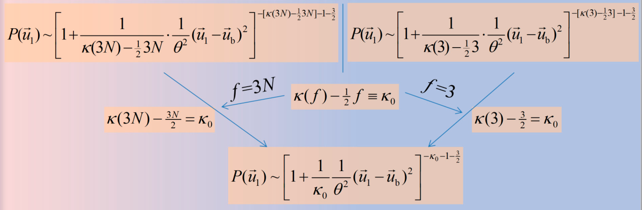
3.2. The Paradox of the 1-Particle Kappa Distribution

Let us consider the N-particle kappa distribution of velocities. If this is integrated over the d-dimensional velocity space of the N^th particle, the result is the (N − 1)-particle kappa distribution of velocities. If this is then integrated over the (N − 1)^th particle velocity, the (N − 2)-particle kappa distribution will be derived, and by continuing the integration over all (N − 1) particle velocities, we end up to the 1-particle distribution. Namely:

$$\begin{array}{l}P({\overrightarrow{u}}_1,{\overrightarrow{u}}_2,\dots ,{\overrightarrow{u}}_{N-2},{\overrightarrow{u}}_{N-1},{\overrightarrow{u}}_N)~{\left[1+\frac{1}{\mathrm{\kappa }-\frac{1}{2}dN}\cdot \frac{1}{{\theta }^2}{\displaystyle \sum _{i=1}^N{({\overrightarrow{u}}_i-{\overrightarrow{u}}_{\mathrm{b}})}^2}\right]}^{-\mathrm{\kappa }-1}\\ \Downarrow \text{integration over}{\overrightarrow{u}}_N\\ P({\overrightarrow{u}}_1,{\overrightarrow{u}}_2,\dots ,{\overrightarrow{u}}_{N-2},{\overrightarrow{u}}_{N-1})~{\left[1+\frac{1}{\mathrm{\kappa }-\frac{1}{2}dN}\cdot \frac{1}{{\theta }^2}{\displaystyle \sum _{i=1}^{N-1}{({\overrightarrow{u}}_i-{\overrightarrow{u}}_{\mathrm{b}})}^2}\right]}^{-\mathrm{\kappa }-1+\frac{1}{2}d}\\ \Downarrow \text{integration over}{\overrightarrow{u}}_{N-1}\\ P({\overrightarrow{u}}_1,{\overrightarrow{u}}_2,\dots ,{\overrightarrow{u}}_{N-2})~{\left[1+\frac{1}{\mathrm{\kappa }-\frac{1}{2}dN}\cdot \frac{1}{{\theta }^2}{\displaystyle \sum _{i=1}^{N-2}{({\overrightarrow{u}}_i-{\overrightarrow{u}}_{\mathrm{b}})}^2}\right]}^{-\mathrm{\kappa }-1+\frac{1}{2}2d}\\ \Downarrow \text{integration over}{\overrightarrow{u}}_{N-2}\\ ⋮\\ \Downarrow \text{integration over}{\overrightarrow{u}}_2\\ P({\overrightarrow{u}}_1)~{\left[1+\frac{1}{\mathrm{\kappa }-\frac{1}{2}dN}\cdot \frac{{({\overrightarrow{u}}_1-{\overrightarrow{u}}_{\mathrm{b}})}^2}{{\theta }^2}\right]}^{-\mathrm{\kappa }-1+\frac{1}{2}d(N-1)}\end{array}$$

Nevertheless, the 1-particle kappa distribution has a different formulation, that is:

$$P({\overrightarrow{u}}_1)~{\left[1+\frac{1}{\mathrm{\kappa }-\frac{1}{2}d}\cdot \frac{1}{{\theta }^2}{({\overrightarrow{u}}_1-{\overrightarrow{u}}_{\mathrm{b}})}^2\right]}^{-\mathrm{\kappa }-1}$$

(14)

and thus, we wonder how these two different formulations can become one:

$$\begin{array}{c}P({\overrightarrow{u}}_1)~{\left[1+\frac{1}{\mathrm{\kappa }-\frac{1}{2}dN}\cdot \frac{1}{{\theta }^2}{({\overrightarrow{u}}_1-{\overrightarrow{u}}_{\mathrm{b}})}^2\right]}^{-\mathrm{\kappa }-1+\frac{1}{2}d(N-1)}\begin{array}{c}?\\ \iff \end{array}\\ P({\overrightarrow{u}}_1)~{\left[1+\frac{1}{\mathrm{\kappa }-\frac{1}{2}d}\cdot \frac{1}{{\theta }^2}{({\overrightarrow{u}}_1-{\overrightarrow{u}}_{\mathrm{b}})}^2\right]}^{-\mathrm{\kappa }-1}\end{array}$$

The problem is solved if we realize that the kappa index is not an invariant quantity, but instead, it depends on the degrees of freedom, κ=κ(f), so that:

$$\begin{array}{c}P({\overrightarrow{u}}_1)~{\left[1+\frac{1}{\mathrm{\kappa }(dN)-\frac{1}{2}dN}\cdot \frac{1}{{\theta }^2}{({\overrightarrow{u}}_1-{\overrightarrow{u}}_{\mathrm{b}})}^2\right]}^{-[\mathrm{\kappa }(dN)-\frac{1}{2}dN]-1-\frac{1}{2}d}\begin{array}{c}?\\ \iff \\ \end{array}\\ P({\overrightarrow{u}}_1)~{\left[1+\frac{1}{\mathrm{\kappa }(d)-\frac{1}{2}d}\cdot \frac{1}{{\theta }^2}{({\overrightarrow{u}}_1-{\overrightarrow{u}}_{\mathrm{b}})}^2\right]}^{-[\mathrm{\kappa }(d)-\frac{1}{2}d]-1-\frac{1}{2}d}\end{array}$$

Hence, it is clear then that there is the following dependence of the kappa index:

$$\mathrm{\kappa }(f)-\frac{1}{2}f=\mathrm{\kappa }(dN)-\frac{1}{2}dN=\mathrm{\kappa }(d)-\frac{1}{2}d\equiv {\mathrm{\kappa }}_0$$

(15)

The kinetic degrees of freedom for the one-particle’s phase space are given by $d\equiv 2<{\mathrm{\epsilon }}_{{\rm K}}>/(k_{\mathrm{B}}T)$, where ${\mathrm{\epsilon }}_{{\rm K}}$ is the particle kinetic energy. As mentioned, κ₀ indicates the kappa index that is invariant of the kinetic degrees of freedom of the system [49]. In contrast to κ₀, the well-known kappa index κ depends on the particle kinetic degrees of freedom d and the number of correlated particles N. Therefore, the quantity κ₀ is a modified kappa index that is not dependent on the dimensionality. Its range of values is (0,∞), with κ₀→∞ corresponding to thermal equilibrium and κ₀→∞ to the furthest state from thermal equilibrium, also called anti-equilibrium.

Using this invariant kappa index, the 1-particle distribution is written with a unified way:

$$P({\overrightarrow{u}}_1)~{\left[1+\frac{1}{{\mathrm{\kappa }}_0}\cdot \frac{1}{{\theta }^2}{({\overrightarrow{u}}_1-{\overrightarrow{u}}_{\mathrm{b}})}^2\right]}^{-{\mathrm{\kappa }}_0-1-\frac{1}{2}d}$$

(16)

while the N-particle distribution becomes:

$$P({\overrightarrow{u}}_1,{\overrightarrow{u}}_2,\dots ,{\overrightarrow{u}}_N)~{\left[1+\frac{1}{{\mathrm{\kappa }}_0}\cdot \frac{1}{{\theta }^2}{\displaystyle \sum _{i=1}^N{({\overrightarrow{u}}_i-{\overrightarrow{u}}_{\mathrm{b}})}^2}\right]}^{-{\mathrm{\kappa }}_0-1-\frac{1}{2}dN}$$

(17)

Finally, Figure 2 summarizes the described paradox and its solution:

4. Formulation of the Kappa Distributions

4.1. Absence of Potential Energy

In the absence of a potential energy, the particle energy is given simply by their kinetic energy. This is the most frequent case in space plasmas analyses. The kappa distribution of velocities is:

$$P(\overrightarrow{u};{\overrightarrow{u}}_b;{\mathrm{\kappa }}_0,T)={(\pi {\mathrm{\kappa }}_0{\theta }^2)}^{-\frac{1}{2}d}\cdot \frac{\mathrm{\Gamma }({\mathrm{\kappa }}_0+1+\frac{1}{2}d)}{\mathrm{\Gamma }({\mathrm{\kappa }}_0+1)}\cdot {\left[1+\frac{1}{{\mathrm{\kappa }}_0}\cdot \frac{{(\overrightarrow{u}-{\overrightarrow{u}}_b)}^2}{{\theta }^2}\right]}^{-{\mathrm{\kappa }}_0-1-\frac{1}{2}d}$$

(18)

The kappa distribution of the kinetic energy, ${\mathrm{\epsilon }}_{\mathrm{K}}=\frac{1}{2}m{(\overrightarrow{u}-{\overrightarrow{u}}_b)}^2$, is given by:

$$P({\mathrm{\epsilon }}_{\mathrm{K}};{\mathrm{\kappa }}_0,T)d{\mathrm{\epsilon }}_{\mathrm{K}}=\frac{{({\mathrm{\kappa }}_0{k}_{\mathrm{B}}T)}^{-\frac{1}{2}d}}{\mathrm{B}(\frac{1}{2}d,{\mathrm{\kappa }}_0+1)}\cdot {\left(1+\frac{1}{{\mathrm{\kappa }}_0}\cdot \frac{{\mathrm{\epsilon }}_{\mathrm{K}}}{k_{\mathrm{B}}T}\right)}^{-{\mathrm{\kappa }}_0-1-\frac{1}{2}d}{\mathrm{\epsilon }}_{\mathrm{K}}{}^{\frac{1}{2}d-1}d{\mathrm{\epsilon }}_{\mathrm{K}}$$

(19)

where ${\rm B}(x,y)\equiv \mathrm{\Gamma }(x)\mathrm{\Gamma }(y)/\mathrm{\Gamma }(x+y)$ is the Beta function. The kinetic energy is expressed in the co-moving system of the flow with bulk velocity ${\overrightarrow{u}}_b$.

4.2. Presence of a Potential Energy

After the connection of empirical kappa distributions with the solid background of non-extensive statistical mechanics [1], it is straightforward now to generalize the distribution from the description of velocities to the description of the Hamiltonian [13]. More specifically, we are able to handle the existence of a non-negligible potential energy using the mathematical formulations and the physical theory of kappa distributions:

$$P(\overrightarrow{r},\overrightarrow{u};\mathrm{\kappa },T)~{\left[1+\frac{1}{\mathrm{\kappa }}\cdot \frac{H(\overrightarrow{r},\overrightarrow{u})-\langle H\rangle }{k_{B}T}\right]}^{-\mathrm{\kappa }-1}$$

(20)

where <H>is the ensemble phase-space average of the Hamiltonian function $H(\overrightarrow{r},\overrightarrow{u})$.

The Hamiltonian function is given by $H(\overrightarrow{r},\overrightarrow{u})={\mathrm{\epsilon }}_{\mathrm{K}}(\overrightarrow{u})+m\mathrm{\Phi }(\overrightarrow{r})$, where ${\mathrm{\epsilon }}_{\mathrm{K}}(\overrightarrow{u})=\frac{1}{2}m{(\overrightarrow{u}-{\overrightarrow{u}}_b)}^2$ is the (velocity dependent) kinetic energy and $m\mathrm{\Phi }(\overrightarrow{r})$ is the (position-dependent) potential energy. Thus, Equation (3) gives:

$$\begin{array}{l}P(\overrightarrow{r},\overrightarrow{u})~{\left\{1+\frac{1}{\mathrm{\kappa }}\cdot \frac{{\mathrm{\epsilon }}_{\mathrm{K}}(\overrightarrow{u})-\langle {\mathrm{\epsilon }}_{\mathrm{K}}(\overrightarrow{u})\rangle +m[\mathrm{\Phi }(\overrightarrow{r})-\langle \mathrm{\Phi }\rangle ]}{k_{\mathrm{B}}T}\right\}}^{-\mathrm{\kappa }-1}\\ ~{\left\{1+\frac{1}{\mathrm{\kappa }-\frac{\langle {\mathrm{\epsilon }}_{\mathrm{K}}(\overrightarrow{u})\rangle }{k_{B}T}}\cdot \frac{{\mathrm{\epsilon }}_{\mathrm{K}}(\overrightarrow{u})+m[\mathrm{\Phi }(\overrightarrow{r})-\langle \mathrm{\Phi }\rangle ]}{k_{\mathrm{B}}T}\right\}}^{-\mathrm{\kappa }-1}={\left\{1+\frac{1}{\mathrm{\kappa }-\frac{1}{2}d}\cdot \frac{{\mathrm{\epsilon }}_{\mathrm{K}}(\overrightarrow{u})+m[\mathrm{\Phi }(\overrightarrow{r})-\langle \mathrm{\Phi }\rangle ]}{k_{\mathrm{B}}T}\right\}}^{-\mathrm{\kappa }-1}.\end{array}$$

Finally, in terms of the invariant kappa index κ₀, the phase-space distribution becomes:

$$P(\overrightarrow{r},\overrightarrow{u};{\overrightarrow{u}}_b;{\mathrm{\kappa }}_0,T)~{\left\{1+\frac{1}{{\mathrm{\kappa }}_0}\cdot \frac{\frac{1}{2}m{(\overrightarrow{u}-{\overrightarrow{u}}_b)}^2+m[\mathrm{\Phi }(\overrightarrow{r})-\langle \mathrm{\Phi }\rangle ]}{k_{B}T}\right\}}^{-{\mathrm{\kappa }}_0-1-\frac{1}{2}d}$$

(21)

What is really important is to derive the marginal probability distributions, which are given by:

$$(\mathrm{i})P(\overrightarrow{r})={\displaystyle {\int }_{-\infty }^{\infty }P(\overrightarrow{r},\overrightarrow{u})d\overrightarrow{u}},(\mathrm{ii})P(\overrightarrow{u})={\displaystyle {\int }_{-\infty }^{\infty }P(\overrightarrow{r},\overrightarrow{u})d\overrightarrow{r}}\text{or}P({\mathrm{\epsilon }}_{\mathrm{K}})={\displaystyle {\int }_{-\infty }^{\infty }P(\overrightarrow{r},{\mathrm{\epsilon }}_{\mathrm{K}})d\overrightarrow{r}}$$

(22)

( $d\overrightarrow{u}$ symbolizes the infinitensimal volume in velocity space). The above derived in (22) are the (i) (marginal) positional kappa distribution, and the (ii) (marginal) kappa distribution of velocity or kinetic energy, respectively.

4.3. Example of Kappa Distributions with Nonzero Potential Energy

As an example of a potential energy, we examine the 1-dimensional linear gravitational potential, $m\mathrm{\Phi }(z)=mgz$, which is dependent on the altitude z. As it was shown in [13], the complete phase-space kappa distribution is given by:

$$P(z,{\mathrm{\epsilon }}_{\mathrm{K}};{\mathrm{\kappa }}_0,T,z_0)d{\mathrm{\epsilon }}_{\mathrm{K}}dz=\frac{\mathrm{\Gamma }({\mathrm{\kappa }}_0+1+\frac{1}{2}d)}{{({\mathrm{\kappa }}_0-1)}^{\frac{1}{2}d+1}\mathrm{\Gamma }(\frac{1}{2}d)\mathrm{\Gamma }({\mathrm{\kappa }}_0)}\cdot {(k_{B}T)}^{-\frac{1}{2}d}{z}_0{}^{-1}\cdot {\left[1+\frac{1}{{\mathrm{\kappa }}_0-1}\cdot \left(\frac{{\mathrm{\epsilon }}_{{\rm K}}}{k_{\mathrm{B}}T}+\frac{z}{z_0}\right)\right]}^{-{\mathrm{\kappa }}_0-1-\frac{1}{2}d}{\mathrm{\epsilon }}_{\mathrm{K}}{}^{\frac{1}{2}d-1}d{\mathrm{\epsilon }}_{\mathrm{K}}dz,$$

(23)

while the positional kappa distribution leads to a generalization of the:

$$P(z;{\mathrm{\kappa }}_0,z_0)dz=\frac{{\mathrm{\kappa }}_0}{{\mathrm{\kappa }}_0-1}\cdot z_0{}^{-1}\cdot {\left(1+\frac{1}{{\mathrm{\kappa }}_0-1}\cdot \frac{z}{z_0}\right)}^{-{\mathrm{\kappa }}_0-1}dz,\text{where}{z}_0=\frac{k_{\mathrm{B}}T}{mg}$$

(24)

The marginal kappa distribution of velocities (kinetic energy) is derived from the integration of Equation (14) over positions:

$$\begin{array}{l}P({\mathrm{\epsilon }}_{\mathrm{K}};{\mathrm{\kappa }}_0,T)={\displaystyle {\int }_0^{\infty }P({\mathrm{\epsilon }}_{\mathrm{K}},z;{\mathrm{\kappa }}_0,T,z_0)dz}=\\ \frac{\mathrm{\Gamma }({\mathrm{\kappa }}_0+1+\frac{1}{2}d)}{{({\mathrm{\kappa }}_0-1)}^{\frac{1}{2}d+1}\mathrm{\Gamma }(\frac{1}{2}d)\mathrm{\Gamma }({\mathrm{\kappa }}_0)}\cdot {(k_{B}T)}^{-\frac{1}{2}d}{z}_0{}^{-1}\cdot {\mathrm{\epsilon }}_{\mathrm{K}}{}^{\frac{1}{2}d-1}\cdot {\displaystyle {\int }_0^{\infty }{\left[1+\frac{1}{{\mathrm{\kappa }}_0-1}\cdot \left(\frac{{\mathrm{\epsilon }}_{{\rm K}}}{k_{\mathrm{B}}T}+\frac{z}{z_0}\right)\right]}^{-{\mathrm{\kappa }}_0-1-\frac{1}{2}d}dz}\end{array}$$

(25)

or:

$$P({\mathrm{\epsilon }}_{\mathrm{K}};{\mathrm{\kappa }}_0,T)=\frac{{[({\mathrm{\kappa }}_0-1)k_{B}T]}^{-\frac{1}{2}d}}{{\rm B}[\frac{1}{2}d,({\mathrm{\kappa }}_0-1)+1]}\cdot {\left[1+\frac{1}{{\mathrm{\kappa }}_0-1}\cdot \frac{{\mathrm{\epsilon }}_{{\rm K}}}{k_{\mathrm{B}}T}\right]}^{-({\mathrm{\kappa }}_0-1)-1-\frac{1}{2}d}{\mathrm{\epsilon }}_{\mathrm{K}}{}^{\frac{1}{2}d-1}$$

(26)

We notice that by applying the transformation ${\mathrm{\kappa }}_0-1\to {\tilde{\mathrm{\kappa }}}_0$:

$$P({\mathrm{\epsilon }}_{\mathrm{K}};{\tilde{\mathrm{\kappa }}}_0,T)=\frac{{({\tilde{\mathrm{\kappa }}}_0{k}_{B}T)}^{-\frac{1}{2}d}}{{\rm B}(\frac{1}{2}d,{\tilde{\mathrm{\kappa }}}_0+1)}\cdot {\left[1+\frac{1}{{\tilde{\mathrm{\kappa }}}_0}\cdot \frac{{\mathrm{\epsilon }}_{{\rm K}}}{k_{\mathrm{B}}T}\right]}^{-{\tilde{\mathrm{\kappa }}}_0-1-\frac{1}{2}d}{\mathrm{\epsilon }}_{\mathrm{K}}{}^{\frac{1}{2}d-1}$$

(27)

which coincides exactly with Equation (10) (more examples on non-zero potential energies can be found in [13]; also, see [63]).

5. The Effect of the Potential Energy on the Kappa and q Indices

We have already seen that the presence of the 1-dimensional linear gravitational potential, $m\mathrm{\Phi }(z)=mgz$, led to the marginal kappa distribution of kinetic energy (26):

$$P({\mathrm{\epsilon }}_{\mathrm{K}};{\mathrm{\kappa }}_0,T)=\frac{{[({\mathrm{\kappa }}_0-1)k_{B}T]}^{-\frac{1}{2}d}}{{\rm B}[\frac{1}{2}d,({\mathrm{\kappa }}_0-1)+1]}\cdot {\left[1+\frac{1}{{\mathrm{\kappa }}_0-1}\cdot \frac{{\mathrm{\epsilon }}_{{\rm K}}}{k_{\mathrm{B}}T}\right]}^{-({\mathrm{\kappa }}_0-1)-1-\frac{1}{2}d}{\mathrm{\epsilon }}_{\mathrm{K}}{}^{\frac{1}{2}d-1}$$

(28)

which is identical to the standard kappa distribution with kappa index ${\mathrm{\kappa }}_0-1\to {\tilde{\mathrm{\kappa }}}_0$:

$$P({\mathrm{\epsilon }}_{\mathrm{K}};{\tilde{\mathrm{\kappa }}}_0,T)={\tilde{\mathrm{\kappa }}}_0{}^{-\frac{1}{2}d-1}\frac{\mathrm{\Gamma }({\tilde{\mathrm{\kappa }}}_0+1+\frac{1}{2}d)}{\mathrm{\Gamma }(\frac{1}{2}d)\mathrm{\Gamma }({\tilde{\mathrm{\kappa }}}_0+1)}\cdot {(k_{B}T)}^{-\frac{1}{2}d}{z}_0{}^{-1}\cdot {\left[1+\frac{1}{{\tilde{\mathrm{\kappa }}}_0}\cdot \frac{{\mathrm{\epsilon }}_{{\rm K}}}{k_{\mathrm{B}}T}\right]}^{-{\tilde{\mathrm{\kappa }}}_0-1-\frac{1}{2}d}{\mathrm{\epsilon }}_{\mathrm{K}}{}^{\frac{1}{2}d-1}$$

(29)

It appears that the presence of this potential energy leads to an additional number of effective degrees of freedom, so that:

$$\mathrm{\kappa }={\mathrm{\kappa }}_0+\frac{1}{2}d+1$$

(30)

Therefore, the phase-space kappa distribution (23) is written as:

$$P(z,{\mathrm{\epsilon }}_{\mathrm{K}};{\mathrm{\kappa }}_0,T,z_0)d{\mathrm{\epsilon }}_{\mathrm{K}}dz=\frac{\mathrm{\Gamma }({\mathrm{\kappa }}_0+2+\frac{1}{2}d)}{{\mathrm{\kappa }}_0{}^{\frac{1}{2}d+1}\mathrm{\Gamma }(\frac{1}{2}d)\mathrm{\Gamma }({\mathrm{\kappa }}_0+1)}\cdot {(k_{B}T)}^{-\frac{1}{2}d}{z}_0{}^{-1}\cdot {\left[1+\frac{1}{{\mathrm{\kappa }}_0}\cdot \left(\frac{{\mathrm{\epsilon }}_{{\rm K}}}{k_{\mathrm{B}}T}+\frac{z}{z_0}\right)\right]}^{-{\mathrm{\kappa }}_0-2-\frac{1}{2}d}{\mathrm{\epsilon }}_{\mathrm{K}}{}^{\frac{1}{2}d-1}d{\mathrm{\epsilon }}_{\mathrm{K}}dz,$$

(31)

while the positional (24) and velocity (kinetic energy) (26) kappa distributions, are written as:

$$P(z;{\mathrm{\kappa }}_0,z_0)dz=\frac{{\mathrm{\kappa }}_0+1}{{\mathrm{\kappa }}_0}\cdot z_0{}^{-1}\cdot {\left(1+\frac{1}{{\mathrm{\kappa }}_0}\cdot \frac{z}{z_0}\right)}^{-{\mathrm{\kappa }}_0-2}dz,\text{where}{z}_0=\frac{k_{\mathrm{B}}T}{mg}$$

(32)

$$P({\mathrm{\epsilon }}_{\mathrm{K}};{\mathrm{\kappa }}_0,T)={\mathrm{\kappa }}_0{}^{-\frac{1}{2}d-1}\frac{\mathrm{\Gamma }({\mathrm{\kappa }}_0+1+\frac{1}{2}d)}{\mathrm{\Gamma }(\frac{1}{2}d)\mathrm{\Gamma }({\mathrm{\kappa }}_0+1)}\cdot {(k_{B}T)}^{-\frac{1}{2}d}{z}_0{}^{-1}\cdot {\left[1+\frac{1}{{\mathrm{\kappa }}_0}\cdot \frac{{\mathrm{\epsilon }}_{{\rm K}}}{k_{\mathrm{B}}T}\right]}^{-{\mathrm{\kappa }}_0-1-\frac{1}{2}d}{\mathrm{\epsilon }}_{\mathrm{K}}{}^{\frac{1}{2}d-1}$$

(33)

Let us now generalize this result. Instead of the 1-dimensional case of z ( $m\mathrm{\Phi }(z)~z$), we assume a potential that depends on r, that is embedded in a d_r-dimensional positional space. Therefore, we examine the potential $m\mathrm{\Phi }(r)=c\cdot r^b$, $r\in {\Re }^{d_r}$. In order to avoid any confusion, we symbolize the dimensionality of the velocity vector with d_u, i.e., $\Vert \overrightarrow{u}\Vert \equiv u\in {\Re }^{d_u}$. Then, the phase-space kappa distribution is given by:

$$\begin{array}{c}P(r,{\mathrm{\epsilon }}_{\mathrm{K}};{\mathrm{\kappa }}_0,T)d{\mathrm{\epsilon }}_{\mathrm{K}}dr=\\ \frac{b\cdot {({\mathrm{\kappa }}_0-\frac{1}{b}{d}_{\mathrm{r}})}^{-(\frac{1}{2}{d}_{\mathrm{u}}+\frac{1}{b}{d}_{\mathrm{r}})}\mathrm{\Gamma }({\mathrm{\kappa }}_0+1+\frac{1}{2}{d}_{\mathrm{u}})}{\mathrm{\Gamma }(\frac{1}{b}{d}_{\mathrm{r}})\mathrm{\Gamma }(\frac{1}{2}{d}_{\mathrm{u}})\mathrm{\Gamma }({\mathrm{\kappa }}_0-\frac{1}{b}{d}_{\mathrm{r}}+1)}\cdot {(k_{B}T)}^{-(\frac{1}{2}{d}_{\mathrm{u}}+\frac{1}{b}{d}_{\mathrm{r}})}{c}^{\frac{1}{b}{d}_{\mathrm{r}}}\cdot {\left(1+\frac{1}{{\mathrm{\kappa }}_0-\frac{1}{b}{d}_{\mathrm{r}}}\cdot \frac{{\mathrm{\epsilon }}_{{\rm K}}+c{r}^b}{k_{\mathrm{B}}T}\right)}^{-{\mathrm{\kappa }}_0-1-\frac{1}{2}{d}_{\mathrm{u}}}{\mathrm{\epsilon }}_{\mathrm{K}}{}^{\frac{1}{2}{d}_{\mathrm{u}}-1}{r}^{d_{\mathrm{r}}-1}d{\mathrm{\epsilon }}_{\mathrm{K}}dr\end{array}$$

(34)

The marginal kappa distributions of positions (radius) and velocities (kinetic energy) are respectively given by:

$$P(r;{\mathrm{\kappa }}_0,T)dr=\frac{b\cdot {({\mathrm{\kappa }}_0-\frac{1}{b}{d}_{\mathrm{r}})}^{-\frac{1}{b}{d}_{\mathrm{r}}}}{{\rm B}(\frac{1}{b}{d}_{\mathrm{r}},{\mathrm{\kappa }}_0-\frac{1}{b}{d}_{\mathrm{r}}+1)}\cdot {(k_{B}T/c)}^{-\frac{1}{b}{d}_{\mathrm{r}}}\cdot {\left(1+\frac{1}{{\mathrm{\kappa }}_0-\frac{1}{b}{d}_{\mathrm{r}}}\cdot \frac{c{r}^b}{k_{\mathrm{B}}T}\right)}^{-{\mathrm{\kappa }}_0-1}{r}^{d_{\mathrm{r}}-1}dr$$

(35)

and:

$$\begin{array}{c}P({\mathrm{\epsilon }}_{\mathrm{K}};{\mathrm{\kappa }}_0,T)d{\mathrm{\epsilon }}_{\mathrm{K}}=\frac{{({\mathrm{\kappa }}_0-\frac{1}{b}{d}_{\mathrm{r}})}^{-\frac{1}{2}{d}_{\mathrm{u}}}}{{\rm B}(\frac{1}{2}{d}_{\mathrm{u}},{\mathrm{\kappa }}_0-\frac{1}{b}{d}_{\mathrm{r}}+1)}\cdot {(k_{B}T)}^{-\frac{1}{2}{d}_{\mathrm{u}}}\cdot {\left(1+\frac{1}{{\mathrm{\kappa }}_0-\frac{1}{b}{d}_{\mathrm{r}}}\cdot \frac{{\mathrm{\epsilon }}_{{\rm K}}}{k_{\mathrm{B}}T}\right)}^{-({\mathrm{\kappa }}_0-\frac{1}{b}{d}_{\mathrm{r}})-1-\frac{1}{2}{d}_{\mathrm{u}}}{\mathrm{\epsilon }}_{\mathrm{K}}{}^{\frac{1}{2}{d}_{\mathrm{u}}-1}d{\mathrm{\epsilon }}_{\mathrm{K}}\\ {\mathrm{\kappa }}_0>\frac{1}{b}{d}_{\mathrm{r}}\end{array}$$

(36)

The distribution of velocities (36) converges for ${\mathrm{\kappa }}_0>0$, while the distribution of positions (35) converges for ${\mathrm{\kappa }}_0>\frac{1}{b}{d}_{\mathrm{r}}$. Substituting ${\mathrm{\kappa }}_0-\frac{1}{b}{d}_{\mathrm{r}}\to {\mathrm{\kappa }}_0$, we have:

$$P({\mathrm{\epsilon }}_{\mathrm{K}};{\mathrm{\kappa }}_0,T)d{\mathrm{\epsilon }}_{\mathrm{K}}=\frac{{\mathrm{\kappa }}_0{}^{-\frac{1}{2}{d}_{\mathrm{u}}}}{{\rm B}(\frac{1}{2}{d}_{\mathrm{u}},{\mathrm{\kappa }}_0+1)}\cdot {(k_{B}T)}^{-\frac{1}{2}{d}_{\mathrm{u}}}\cdot {\left(1+\frac{1}{{\mathrm{\kappa }}_0}\cdot \frac{{\mathrm{\epsilon }}_{{\rm K}}}{k_{\mathrm{B}}T}\right)}^{-{\mathrm{\kappa }}_0-1-\frac{1}{2}{d}_{\mathrm{u}}}{\mathrm{\epsilon }}_{\mathrm{K}}{}^{\frac{1}{2}{d}_{\mathrm{u}}-1}d{\mathrm{\epsilon }}_{\mathrm{K}}{\mathrm{\kappa }}_0>0,$$

(37)

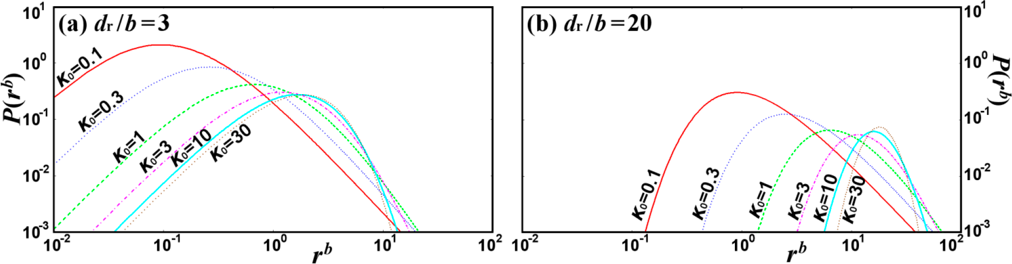
that is identical to the standard kappa distribution of kinetic energy (19). The positional distribution is:

$$P(r;{\mathrm{\kappa }}_0,T)dr=\frac{b\cdot {\mathrm{\kappa }}_0{}^{-\frac{1}{b}{d}_{\mathrm{r}}}}{{\rm B}(\frac{1}{b}{d}_{\mathrm{r}},{\mathrm{\kappa }}_0+1)}\cdot {(k_{B}T/c)}^{-\frac{1}{b}{d}_{\mathrm{r}}}\cdot {\left(1+\frac{1}{{\mathrm{\kappa }}_0}\cdot \frac{c{r}^b}{k_{\mathrm{B}}T}\right)}^{-{\mathrm{\kappa }}_0-1-\frac{1}{b}{d}_{\mathrm{r}}}{r}^{d_{\mathrm{r}}-1}dr$$

(38)

In Figure 3 we plot the function:

$$P(r^b;{\mathrm{\kappa }}_0)dr=\frac{{\mathrm{\kappa }}_0{}^{-\frac{1}{b}{d}_{\mathrm{r}}}}{{\rm B}(\frac{1}{b}{d}_{\mathrm{r}},{\mathrm{\kappa }}_0+1)}\cdot {\left(1+\frac{1}{{\mathrm{\kappa }}_0}\cdot r^b\right)}^{-{\mathrm{\kappa }}_0-1-\frac{1}{b}{d}_{\mathrm{r}}}{(r^b)}^{d_{\mathrm{r}}/b-1}d(r^b)$$

(39)

where the radial distance is in units of ${(k_{B}T/c)}^{1/b}$.

The respective phase-space distribution is:

$$\begin{array}{c}P(r,{\mathrm{\epsilon }}_{\mathrm{K}};{\mathrm{\kappa }}_0,T)d{\mathrm{\epsilon }}_{\mathrm{K}}dr=\\ \frac{b\cdot {\mathrm{\kappa }}_0{}^{-(\frac{1}{2}{d}_{\mathrm{u}}+\frac{1}{b}{d}_{\mathrm{r}})}\mathrm{\Gamma }({\mathrm{\kappa }}_0+1+\frac{1}{2}{d}_{\mathrm{u}}+\frac{1}{b}{d}_{\mathrm{r}})}{\mathrm{\Gamma }(\frac{1}{b}{d}_{\mathrm{r}})\mathrm{\Gamma }(\frac{1}{2}{d}_{\mathrm{u}})\mathrm{\Gamma }({\mathrm{\kappa }}_0+1)}\cdot {(k_{B}T)}^{-(\frac{1}{2}{d}_{\mathrm{u}}+\frac{1}{b}{d}_{\mathrm{r}})}{c}^{\frac{1}{b}{d}_{\mathrm{r}}}\cdot {\left(1+\frac{1}{{\mathrm{\kappa }}_0}\cdot \frac{{\mathrm{\epsilon }}_{{\rm K}}+c{r}^b}{k_{\mathrm{B}}T}\right)}^{-{\mathrm{\kappa }}_0-1-\frac{1}{2}{d}_{\mathrm{u}}-\frac{1}{b}{d}_{\mathrm{r}}}{\mathrm{\epsilon }}_{\mathrm{K}}{}^{\frac{1}{2}{d}_{\mathrm{u}}-1}{r}^{d_{\mathrm{r}}-1}d{\mathrm{\epsilon }}_{\mathrm{K}}dr\end{array}$$

(40)

Therefore, the kappa index depends not only on the dimensionality of the velocity space, but also, on the dimensionality of the positional space. The dependence is similar for both spaces, namely:

$$\mathrm{\kappa }=\text{constant}+\frac{1}{2}{d}_{\mathrm{u}}+\frac{1}{b}{d}_{\mathrm{r}}=\text{constant}+\frac{\langle {\mathrm{\epsilon }}_{{\rm K}}\rangle }{k_{\mathrm{B}}T}+\frac{\langle m\mathrm{\Phi }\rangle }{k_{\mathrm{B}}T}=\text{constant}+\frac{\langle H\rangle }{k_{\mathrm{B}}T}$$

(41)

The constant defines the invariant kappa index, κ₀, which is independent of the positional and kinetic degrees of freedom, with a range of values ${\mathrm{\kappa }}_0\in (0,\infty )$. This is similar to the definition of κ₀ in Equation (6), but now we have included also the effect of the potential energy. Hence, we have:

$$\mathrm{\kappa }={\mathrm{\kappa }}_0+(\frac{1}{2}{d}_{\mathrm{u}}+\frac{1}{b}{d}_{\mathrm{r}})N$$

(42)

6. Discussion: Problems of Non-Extensive Statistical Mechanics and their Resolution through the Kappa Index Dependence on the Degrees of Freedom

6.1. Correlation: Independent of the Total Number of Particles

The origin of the vastly different statistical behavior between classical particle systems and space plasmas is the manifestation of local correlations between the plasma particles. The stronger the correlation the furthest the plasma resides from thermal equilibrium [49]. While correlations shift plasmas away from thermal equilibrium, collisions destroy correlations, recovering plasmas back at thermal equilibrium [64]. Certainly, there may be various and different mechanisms of creating kappa distributions in space and other plasmas, e.g., the presence of weak turbulence [21] and pick-up ions [20,65]. Nevertheless, the reason why kappa distributions exist and sustain themselves in space plasmas is the presence of correlations in collisionless environment. The variance-covariance between the energies of any two particles are given by:

$$\langle {\overrightarrow{u}}_{(n)}{}^2\cdot {\overrightarrow{u}}_{(m)}{}^2\rangle ={\theta }^4\cdot \frac{{\mathrm{\kappa }}_0}{{\mathrm{\kappa }}_0-1}\times \{\begin{array}{l}{\left(\frac{d}{2}\right)}^2\text{if}n\ne m,\\ \left(\frac{d}{2}\right)\cdot \left(\frac{d}{2}+1\right)\text{if}n=m,\end{array}$$

(43)

or:

$$\langle {\mathrm{\epsilon }}_{{\rm K}}{}_{(n)}\cdot {\mathrm{\epsilon }}_{{\rm K}}{}_{(m)}\rangle ={(k_{{\rm B}}T)}^2\cdot \frac{{\mathrm{\kappa }}_0}{{\mathrm{\kappa }}_0-1}\times \{\begin{array}{l}{\left(\frac{d}{2}\right)}^2\text{if}n\ne m,\\ \left(\frac{d}{2}\right)\cdot \left(\frac{d}{2}+1\right)\text{if}n=m.\end{array}$$

(44)

Therefore, the correlation of the energies of two particles is found [49] to be:

$$\rho ({\mathrm{\kappa }}_0;d)=\frac{\langle {\mathrm{\epsilon }}_{(n)}\cdot {\mathrm{\epsilon }}_{(m)}\rangle -\langle {\mathrm{\epsilon }}_{(n)}\rangle \cdot \langle {\mathrm{\epsilon }}_{(m)}\rangle }{\sqrt{\langle {\mathrm{\epsilon }}_{(n)}{}^2\rangle -{\langle {\mathrm{\epsilon }}_{(n)}\rangle }^2}\cdot \sqrt{\langle {\mathrm{\epsilon }}_{(m)}{}^2\rangle -{\langle {\mathrm{\epsilon }}_{(m)}\rangle }^2}}=\frac{\frac{1}{2}d}{{\mathrm{\kappa }}_0+\frac{1}{2}d}$$

(45)

For particles with different degrees of freedom, the respective relations are:

$$\langle {\overrightarrow{u}}_{(n)}{}^2\cdot {\overrightarrow{u}}_{(m)}{}^2\rangle ={\theta }^4\cdot \frac{{\mathrm{\kappa }}_0}{{\mathrm{\kappa }}_0-1}\times \{\begin{array}{l}\left(\frac{d_{(n)}}{2}\right)\cdot \left(\frac{d_{(m)}}{2}\right)\text{if}n\ne m,\\ \left(\frac{d_{(n)}}{2}\right)\cdot \left(\frac{d_{(n)}}{2}+1\right)\text{if}n=m,\end{array}$$

(46)

or in terms of energy:

$$\langle {\mathrm{\epsilon }}_{(n)}\cdot {\mathrm{\epsilon }}_{(m)}\rangle ={(k_{{\rm B}}T)}^2\cdot \frac{{\mathrm{\kappa }}_0}{{\mathrm{\kappa }}_0-1}\times \{\begin{array}{l}\left(\frac{d_{(n)}}{2}\right)\cdot \left(\frac{d_{(m)}}{2}\right)\text{if}n\ne m,\\ \left(\frac{d_{(n)}}{2}\right)\cdot \left(\frac{d_{(n)}}{2}+1\right)\text{if}n=m.\end{array}$$

(47)

Then, the correlation between these different particles is given by

$$\rho ({\mathrm{\kappa }}_0;d_{(n)},d_{(m)})=\sqrt{\frac{\frac{1}{2}{d}_{(n)}}{{\mathrm{\kappa }}_0+\frac{1}{2}{d}_{(n)}}}\cdot \sqrt{\frac{\frac{1}{2}{d}_{(m)}}{{\mathrm{\kappa }}_0+\frac{1}{2}{d}_{(m)}}}=\sqrt{\rho ({\mathrm{\kappa }}_0;d_{(n)})\cdot \rho ({\mathrm{\kappa }}_0;d_{(m)})}$$

(48)

In terms of the variant kappa index, which depends on the degrees of freedom, $\mathrm{\kappa }={\mathrm{\kappa }}_0+\frac{1}{2}dN$, the correlation is written as:

$$\rho (\mathrm{\kappa };d)=\frac{\frac{1}{2}d}{\mathrm{\kappa }-\frac{1}{2}d(N-1)}$$

(49)

or in terms of the q-index:

$$\rho (q;d)=\frac{(q-1)d}{2+(1-q)d(N-1)}$$

(50)

This was the result found first by [66]. One of the strange consequences of this result is that the correlation between two particles decreases with the number of (correlated) particles; in fact, when N→∞, the correlation vanishes, ρ→∞. But the correlation between two particles should not be dependent on the number of other particles. The worst paradox is that, we find again that the value of the kappa index must be large. Namely, for $0\le \rho (\mathrm{\kappa };d)\le 1$ we obtain $\frac{1}{2}dN\le \mathrm{\kappa }$. On the other hand, for $-1\le \rho (\mathrm{\kappa };d)\le 0$, we have $\mathrm{\kappa }\le \frac{1}{2}d(N-2)$, i.e., the kappa index cannot be infinity, which is necessary property of non-extensive statistical mechanics to include systems that recover at equilibrium and BG statistical mechanics.

Note that using the invariant kappa index and its interpretation as inverse to correlation, we can classify the types of systems in an arrangement called, the κ-spectrum (Figure 4).

6.2. The Problem of Divergence

One of the major issues in the formalism of non-extensive statistical mechanics is the multiple integrations of the canonical distribution (in terms of the kinetic energy or the velocities). As was shown in Section 3, each of the integrations contributes to the exponent by adding $\frac{1}{2}d$. Hence, (N − 1) multiple integrations of the velocity of the (N − 1) particles, increase the exponent by $\frac{1}{2}d\cdot (N-1)$; then, the whole exponent becomes $-(\mathrm{\kappa }-\frac{1}{2}d\cdot N)-1-\frac{1}{2}d$, and the whole 1-particle distribution is:

$$P({\overrightarrow{u}}_1)~{\left[1+\frac{1}{\mathrm{\kappa }-\frac{1}{2}dN}\cdot \frac{1}{{\theta }^2}{({\overrightarrow{u}}_1-{\overrightarrow{u}}_{\mathrm{b}})}^2\right]}^{-(\mathrm{\kappa }-\frac{1}{2}dN)-1-\frac{1}{2}d}$$

(51)

The integral of the mean kinetic energy (2nd statistical moment of velocity at the co-moving frame) must converge (so that the temperature to be defined). For this, the asymptotic behavior at infinity of $u_1{}^{2}P({\overrightarrow{u}}_1)u_1{}^{d-1}$ must be falling faster than a power law of $u_1{}^{-1}$. We have:

$$u_1{}^{2}P({\overrightarrow{u}}_1)u_1{}^{d-1}~u_1{}^2{\left[1+\frac{1}{\mathrm{\kappa }-\frac{1}{2}dN}\cdot \frac{1}{{\theta }^2}{({\overrightarrow{u}}_1-{\overrightarrow{u}}_{\mathrm{b}})}^2\right]}^{-(\mathrm{\kappa }-\frac{1}{2}dN)-1-\frac{1}{2}d}{u}_1{}^{d-1}\stackrel{u_1\to \infty }{\to }{u}_1{}^2{u}_1{}^{-2(\mathrm{\kappa }-\frac{1}{2}dN)-2-d}{u}_1{}^{d-1}~u_1{}^{-2(\mathrm{\kappa }-\frac{1}{2}dN)-1}$$

or $-2(\mathrm{\kappa }-\frac{1}{2}dN)-1<-1$, from which we obtain the range of the allowable values of the kappa or q- indices, that is:

$$\mathrm{\kappa }>\frac{1}{2}dN\text{or}q<1+1/(\frac{1}{2}dN)$$

(52)

while for indices out of this range, $\mathrm{\kappa }\le \frac{1}{2}dN$ or $q\ge 1+1/(\frac{1}{2}dN)$, the integrals diverge and the distributions cannot be normalized.

Given the large number of particles, practically N→∞, we obviously find that κ→∞ or q→1, which corresponds to the limit of non-extensive statistical mechanics to the classical BG statistical mechanics. Therefore, in contrast to our experience from space and other laboratory plasma observation, here we find that non-extensive statistical mechanics is not applicable (!) in the continuous phase spaces with Hamiltonian $H(\overrightarrow{u})={\mathrm{\epsilon }}_{\mathrm{K}}(\overrightarrow{u})=\frac{1}{2}m{(\overrightarrow{u}-{\overrightarrow{u}}_b)}^2$ or $H(\overrightarrow{r},\overrightarrow{u})={\mathrm{\epsilon }}_{\mathrm{K}}(\overrightarrow{u})+m\mathrm{\Phi }(\overrightarrow{r})$.

This paradox is easily resolved when we take into account the dependence of the kappa index on the degrees of freedom. In this case, we have $\mathrm{\kappa }={\mathrm{\kappa }}_0+\frac{1}{2}dN$, hence, the restriction (52) now becomes κ₀>0. (It is interesting to note that the paradox can be resolved only if the kappa index has this specific relation to the degrees of freedom. Also, the number N now corresponds to the correlated number of particles instead of the total number of particles in the system.)

The N-particle kappa distribution of velocities is now written as:

$$P({\overrightarrow{u}}_1,{\overrightarrow{u}}_2,\dots ,{\overrightarrow{u}}_N;{\overrightarrow{u}}_b;{\mathrm{\kappa }}_0,T)={(\pi {\mathrm{\kappa }}_0{\theta }^2)}^{-\frac{1}{2}dN}\cdot \frac{\mathrm{\Gamma }({\mathrm{\kappa }}_0+1+\frac{1}{2}dN)}{\mathrm{\Gamma }({\mathrm{\kappa }}_0+1)}\cdot {\left[1+\frac{1}{{\mathrm{\kappa }}_0}\cdot \frac{1}{{\theta }^2}{\displaystyle \sum _{i=1}^N{({\overrightarrow{u}}_i-{\overrightarrow{u}}_{\mathrm{b}})}^2}\right]}^{-{\mathrm{\kappa }}_0-1-\frac{1}{2}dN}$$

(53)

The N-particle kappa distribution of the kinetic energies, ${\mathrm{\epsilon }}_{\mathrm{K}}{}_i=\frac{1}{2}m{({\overrightarrow{u}}_i-{\overrightarrow{u}}_b)}^2$, is given by:

$$P({\mathrm{\epsilon }}_{\mathrm{K}}{}_1,{\mathrm{\epsilon }}_{\mathrm{K}}{}_2,\dots ,{\mathrm{\epsilon }}_{\mathrm{K}}{}_N;{\mathrm{\kappa }}_0,T)=\frac{{({\mathrm{\kappa }}_0{k}_{\mathrm{B}}T)}^{-\frac{1}{2}dN}\mathrm{\Gamma }({\mathrm{\kappa }}_0+1+\frac{1}{2}dN)}{\mathrm{\Gamma }{(\frac{1}{2}d)}^N\mathrm{\Gamma }({\mathrm{\kappa }}_0+1)}\cdot {\left(1+\frac{1}{{\mathrm{\kappa }}_0}\cdot \frac{1}{k_{\mathrm{B}}T}{\displaystyle \sum _{i=1}^N{\mathrm{\epsilon }}_{\mathrm{K}}{}_i}\right)}^{-{\mathrm{\kappa }}_0-1-\frac{1}{2}dN}{\displaystyle \prod _{i=1}^N{\mathrm{\epsilon }}_{\mathrm{K}}{{}_i}^{\frac{1}{2}d-1}}$$

(54)

but it is more convenient to express the distribution in terms of the total energy ${\mathrm{\epsilon }}_{\mathrm{t}}={\displaystyle {\sum }_{i=1}^N{\mathrm{\epsilon }}_{\mathrm{K}}{}_i}$:

$$P({\mathrm{\epsilon }}_{\mathrm{t}};{\mathrm{\kappa }}_0,T)=\frac{{({\mathrm{\kappa }}_0{k}_{\mathrm{B}}T)}^{-\frac{1}{2}dN}}{\mathrm{B}(\frac{1}{2}dN,{\mathrm{\kappa }}_0+1)}\cdot {\left(1+\frac{1}{{\mathrm{\kappa }}_0}\cdot \frac{{\mathrm{\epsilon }}_{\mathrm{t}}}{k_{\mathrm{B}}T}\right)}^{-{\mathrm{\kappa }}_0-1-\frac{1}{2}dN}{\mathrm{\epsilon }}_{\mathrm{t}}{}^{\frac{1}{2}dN-1}$$

(55)

or the sampling average energy $\overline{\mathrm{\epsilon }}={\mathrm{\epsilon }}_{\mathrm{t}}/N=(1/N)\cdot {\displaystyle {\sum }_{i=1}^N{\mathrm{\epsilon }}_{\mathrm{K}}{}_i}$:

$$P(\overline{\mathrm{\epsilon }};{\mathrm{\kappa }}_0,T)=\frac{{({\mathrm{\kappa }}_0{k}_{\mathrm{B}}T/N)}^{-\frac{1}{2}dN}}{\mathrm{B}(\frac{1}{2}dN,{\mathrm{\kappa }}_0+1)}\cdot {\left(1+\frac{1}{{\mathrm{\kappa }}_0}\cdot \frac{N\overline{\mathrm{\epsilon }}}{k_{\mathrm{B}}T}\right)}^{-{\mathrm{\kappa }}_0-1-\frac{1}{2}dN}{\overline{\mathrm{\epsilon }}}^{\frac{1}{2}dN-1}$$

(56)

which at the limit of $N\to \infty$ becomes:

$$P(\overline{\mathrm{\epsilon }};{\mathrm{\kappa }}_0,T)=\frac{{(\frac{1}{2}d{\mathrm{\kappa }}_0{k}_{\mathrm{B}}T)}^{{\mathrm{\kappa }}_0+1}}{\mathrm{\Gamma }({\mathrm{\kappa }}_0+1)}\cdot \exp \left(-\frac{\frac{1}{2}d{\mathrm{\kappa }}_0{k}_{\mathrm{B}}T}{\overline{\mathrm{\epsilon }}}\right){\overline{\mathrm{\epsilon }}}^{-{\mathrm{\kappa }}_0-2}$$

(57)

or:

$$P(\beta ;{\mathrm{\kappa }}_0)=\frac{{({\mathrm{\kappa }}_0+1)}^{{\mathrm{\kappa }}_0+1}}{\mathrm{\Gamma }({\mathrm{\kappa }}_0+1)}\cdot {\beta }^{({\mathrm{\kappa }}_0+1)-1}\cdot e^{-({\mathrm{\kappa }}_0+1)\beta },\beta \equiv \frac{{\mathrm{\kappa }}_0}{{\mathrm{\kappa }}_0+1}\cdot \frac{\langle \mathrm{\epsilon }\rangle }{\overline{\mathrm{\epsilon }}}$$

(58)

(with $\langle \mathrm{\epsilon }\rangle =\frac{1}{2}d{k}_{\mathrm{B}}T$). Equation (58) reads the well-known distribution of reduced chi-square ${\chi }_{red}^2={\chi }_{}^2/d_0$ for degrees of freedom d₀:

$$P({\chi }_{red}^2;d_0)d{\chi }_{red}^2=\frac{{(\frac{1}{2}{d}_0)}^{\frac{1}{2}{d}_0}}{\mathrm{\Gamma }(\frac{1}{2}{d}_0)}\cdot {({\chi }_{red}^2)}^{\frac{1}{2}{d}_0-1}\cdot e^{-\frac{1}{2}{d}_0({\chi }_{red}^2)}d{\chi }_{red}^2$$

(59)

where we identify the invariant kappa index as:

$${\mathrm{\kappa }}_0=\frac{1}{2}(d_0-2)$$

(60)

Let’s show another example of the hypothetical divergence of non-extensive statistical mechanics, and how the above consideration resolves the problem [69] had studied the problem of divergence in the system of N linear harmonic oscillators. The potential energy of this system is expressed in squared terms of the position, $m\mathrm{\Phi }=c\cdot r^2$, similar to the kinetic energy that is squared terms of the velocity, ${\mathrm{\epsilon }}_{\mathrm{K}}=\frac{1}{2}m\cdot u^2$ (for simplicity and without any loss of the generality, we assume ${\overrightarrow{u}}_b\equiv <\overrightarrow{u}>=0$). Therefore, the total energy is $U={\mathrm{\epsilon }}_{\mathrm{K}}+m\mathrm{\Phi }=\frac{1}{2}m\cdot u^2+c\cdot r^2$, which can be considered a single square term with dimensionality $d_{\mathrm{u}}+d_{\mathrm{r}}$. Hence, the distribution of the total energy behaves similar to Equation (52):

$$P(U;{\mathrm{\kappa }}_0,T)=\frac{{({\mathrm{\kappa }}_0{k}_{\mathrm{B}}T)}^{-\frac{1}{2}dN}}{\mathrm{B}(\frac{1}{2}dN,{\mathrm{\kappa }}_0+1)}\cdot {\left(1+\frac{1}{{\mathrm{\kappa }}_0}\cdot \frac{U}{k_{\mathrm{B}}T}\right)}^{-{\mathrm{\kappa }}_0-1-\frac{1}{2}dN}{U}^{\frac{1}{2}dN-1},\text{with}d=d_{\mathrm{u}}+d_{\mathrm{r}}$$

(61)

For the temperature to exist, the mean energy must converge and thus, we obtain the usual result κ₀>0 However, if the dependence of the kappa index on the degrees of freedom is ignored, the same problem of divergence occurs:

$$P(U;{\mathrm{\kappa }}_0,T)~{\left(1+\frac{1}{{\mathrm{\kappa }}_0}\cdot \frac{U}{k_{\mathrm{B}}T}\right)}^{-\mathrm{\kappa }-1}{U}^{\frac{1}{2}dN}~U^{\frac{1}{2}dN-\mathrm{\kappa }-1}$$

(62)

from where we deduce that the divergence can be avoided only if $\frac{1}{2}dN<\mathrm{\kappa }$, i.e., if d_u=d_r=3, then d=6 and 6N<κ, a result that cannot be used in the framework of non-extensive statistical mechanics, since N can be a large number of collected oscillators, and thus, the kappa index is practically infinity, leading to the BG statistics. The problem of divergence in the system of linear harmonic oscillators has been detected by [69]; here we show how it is resolved given the dependence of κ- and q- indices on the degrees of freedom:

$$\mathrm{\kappa }={\mathrm{\kappa }}_0+(\frac{1}{2}{d}_{\mathrm{u}}+\frac{1}{b}{d}_{\mathrm{r}})N,q=1+{[{\mathrm{\kappa }}_0+(\frac{1}{2}{d}_{\mathrm{u}}+\frac{1}{b}{d}_{\mathrm{r}})N]}^{-1}$$

(63)

7. Conclusions

The paper showed the dependence of the kappa index (or the entropic q-index) on the degrees of freedom, that is, the number of correlated particles, and the per particle kinetic/potential degrees of freedom. First we show this dependence in the case of particle populations described by kappa distributions in the absence of a potential energy. Then, the result is extended in the presence of a potential energy.

It has been shown that the kappa index, κ, has a very simple relation with the degrees of freedom, that is, $\mathrm{\kappa }={\mathrm{\kappa }}_0+(\frac{1}{2}{d}_{\mathrm{u}}+\frac{1}{b}{d}_{\mathrm{r}})N$, where $d_{\mathrm{u}}$ are the kinetic and $d_{\mathrm{r}}$ the potential degrees of freedom (for a potential with polynomial order b around its minimum). The constant ${\mathrm{\kappa }}_0$ denotes the invariant kappa index, which is independent of the degrees of freedom. The respective dependence of the q-index is derived from the connection relation $q=1+1/\mathrm{\kappa }$.

It is shown that various problems of non-extensive statistical mechanics, such as (i) the correlation dependence on the total number of particles; and (ii) the normalization divergence for finite kappa indices, are resolved considering the kappa index dependence on the degrees of freedom.

References

- Livadiotis, G.; McComas, D.J. Beyond kappa distributions: Exploiting Tsallis statistical mechanics in space plasmas. J. Geophys. Res. 2009, 114, A11105. [Google Scholar]
- Livadiotis, G.; McComas, D.J. Understanding Kappa Distributions: A Toolbox for Space Science and Astrophysics. Space Sci. Rev. 2013, 175, 183–214. [Google Scholar]
- Livadiotis, G. “Lagrangian temperature”: Derivation and physical meaning for systems described by kappa distributions. Entropy 2014, 16, 4290–4308. [Google Scholar]
- Livadiotis, G. Statistical background and properties of kappa distributions in space plasmas. J. Geophys. Res. 2015, 120. [Google Scholar] [CrossRef]
- Livadiotis, G.; McComas, D.J. Non-equilibrium thermodynamic processes: Space plasmas and the inner heliosheath. Astrophys. J 2012, 749. [Google Scholar] [CrossRef]
- Livadiotis, G.; McComas, D.J. Evidence of large scale phase-space quantization in plasmas. Entropy 2013, 15, 1116–1132. [Google Scholar]
- Livadiotis, G.; McComas, D.J. Fitting method based on correlation maximization: Applications in space physics. J. Geophys. Res. 2013, 118, 2863–2875. [Google Scholar]
- Livadiotis, G.; McComas, D.J.; Dayeh, M.A.; Funsten, H.O.; Schwadron, N.A. First sky map of the inner heliosheath temperatures using IBEX spectra. Astrophys. J 2011, 734. [Google Scholar] [CrossRef]
- Livadiotis, G.; McComas, D.J.; Randol, B.; Mӧbius, E.; Dayeh, M.A.; Frisch, P.C.; Funsten, H.O.; Schwadron, N.A.; Zank, G.P. Pick-up ion distributions and their influence on energetic neutral atom spectral curvature. Astrophys. J 2012, 751. [Google Scholar] [CrossRef]
- Livadiotis, G.; McComas, D.J.; Schwadron, N.A.; Funsten, H.O.; Fuselier, S.A. Pressure of the proton plasma in the inner heliosheath. Astrophys. J 2013, 762. [Google Scholar] [CrossRef]
- Štverák, S.; Maksimovic, M.; Trávníček, P.M.; Marsch, E.; Fazakerley, A.N.; Scime, E.E. Radial evolution of nonthermal electron populations in the low-latitude solar wind: Helios, Cluster, and Ulysses Observations. J. Geophys. Res. 2009, 114, A05104. [Google Scholar]
- Pierrard, V.; Lazar, M. Kappa distributions: Theory and applications in space plasmas. Sol. Phys. 2010, 267, 153–174. [Google Scholar]
- Livadiotis, G. Kappa distribution in the presence of a potential energy. J. Geophys. Res. 2015, 120, 880–903. [Google Scholar]
- Collier, M.R.; Hamilton, D.C.; Gloeckler, G.; Bochsler, P.; Sheldon, R.B. Neon-20, oxygen-16, and helium-4 densities, temperatures, and suprathermal tails in the solar wind determined with WIND/MASS. Geophys. Res. Lett. 1996, 23, 1191–1194. [Google Scholar]
- Mann, G.; Classen, H.T.; Keppler, E.; Roelof, E.C. On electron acceleration at CIR related shock waves. Astron. Astrophys. 2002, 391, 749–756. [Google Scholar]
- Leubner, M.P. Fundamental issues on kappa-distributions in space plasmas and interplanetary proton distributions. Phys. Plasmas. 2004, 11, 1308–1316. [Google Scholar]
- Maksimovic, M.; Zouganelis, I.; Chaufray, J.-Y.; Issautier, K.; Scime, E.E.; Littleton, J.E.; Marsch, E.; McComas, D.J.; Salem, C.; Lin, R.P.; et al. Radial evolution of the electron distribution functions in the fast solar wind between 0.3 and 1.5 AU. J. Geophys. Res. 2005, 110, A09104. [Google Scholar]
- Marsch, E. Kinetic physics of the solar corona and solar wind. Living Rev. Sol. Phys. 2006, 3, 1–100. [Google Scholar]
- Zouganelis, I. Measuring suprathermal electron parameters in space plasmas: Implementation of the quasi-thermal noise spectroscopy with kappa distributions using in situ Ulysses/URAP radio measurements in the solar wind. J. Geophys. Res. 2008, 113, A08111. [Google Scholar]
- Livadiotis, G.; McComas, D.J. Exploring transitions of space plasmas out of equilibrium. Astrophys. J 2010, 714, 971–987. [Google Scholar]
- Yoon, P.H. Electron kappa distribution and quasi-thermal noise. J. Geophys. Res. 2014, 119, 7074–7087. [Google Scholar]
- Owocki, S.P.; Scudder, J.D. The effect of a non-Maxwellian electron distribution on oxygen and iron ionization balances in the solar corona. Astrophys. J 1983, 270, 758–768. [Google Scholar]
- Vocks, C.; Mann, G.; Rausche, G. Formation of suprathermal electron distributions in the quiet solar corona. Astron. Astrophys. 2008, 480, 527–536. [Google Scholar]
- Lee, E.; Williams, D.R.; Lapenta, G. Spectroscopic Indication of Suprathermal Ions in the Solar Corona; Cornell University: Ithaca, NY, USA, 2013. [Google Scholar]
- Cranmer, S.R. Suprathermal electrons in the solar corona: Can nonlocal transport explain heliospheric charge states? Astrophys. J. Lett. 2014, 791. [Google Scholar] [CrossRef]
- Xiao, F.; Zhou, Q.; Li, C.; Cai, A. Modeling solar energetic particle by a relativistic kappa-type distribution. Plasma Phys. Control. Fusion. 2008, 50, 062001. [Google Scholar]
- Laming, J.M.; Moses, J.D.; Ko, Y.-K.; Ng, C.K.; Rakowski, C.E.; Tylka, A.J. On the remote detection of suprathermal ions in the solar corona and their role as seeds for solar energetic particle production. Astrophys. J 2013, 770. [Google Scholar] [CrossRef]
- Chotoo, K.; Schwadron, N.A.; Mason, G.M.; Zurbuchen, T.H.; Gloeckler, G.; Posner, A.; Fisk, L.A.; Galvin, A.B.; Hamilton, D.C.; Collier, M.R. The suprathermal seed population for corotating interaction region ions at 1 AU deduced from composition and spectra of H+, He++, and He+ observed by wind. J. Geophys. Res. 2000, 105, 23107–23122. [Google Scholar]
- Vasyliũnas, V.M. A survey of low-energy electrons in the evening sector of the magnetosphere with OGO 1 and OGO 3. J. Geophys. Res. 1968, 73, 2839–2884. [Google Scholar]
- Olbert, S. Summary of experimental results from M.I.T. detector on IMP-1. Phys. Magnetosph. 1968, 10, 641–659. [Google Scholar]
- Formisano, V.; Moreno, G.; Palmlotto, F.; Hedgecock, P.C. Solar wind interaction with the Earth’s magnetic field: 1. Magnetosheath. J. Geophys. Res. 1973, 78, 3714–3730. [Google Scholar]
- Ogasawara, K.; Angelopoulos, V.; Dayeh, M.A.; Fuselier, S.A.; Livadiotis, G.; McComas, D.J.; McFadden, J.P. Characterizing the dayside magnetosheath using energetic neutral atoms: IBEX and THEMIS observations. J. Geophys. Res. 2013, 118, 3126–3137. [Google Scholar]
- Grabbe, C. Generation of Broadband Electrostatic Waves in Earth’s Magnetotail. Phys. Rev. Lett. 2000, 84, 3614–3617. [Google Scholar]
- Pisarenko, N.F.; Budnika, E. Yu.; Ermolaev, Yu. I.; Kirpichev, I.P.; Lutsenko, V.N.; Morozova, E.I.; Antonova, E.E. The ion differential spectra in outer boundary of the ring current: November 17, 1995 case study. J. Atmos. Sol. Terrestrial. Phys. 2002, 64, 573–583. [Google Scholar]
- Christon, S.P. A comparison of the Mercury and Earth magnetospheres: Electron measurements and substorm time scales. Icarus 1987, 71, 448–471. [Google Scholar]
- Wang, C.-P.; Lyons, L.R.; Chen, M.W.; Wolf, R.A.; Toffoletto, F.R. Modeling the inner plasma sheet protons and magnetic field under enhanced convection. J. Geophys. Res. 2003, 108, 1074. [Google Scholar]
- Kletzing, C.A.; Scudder, J.D.; Dors, E.E.; Curto, C. Auroral source region: Plasma properties of the high-latitude plasma sheet. J. Geophys. Res. 2003, 108, 1360. [Google Scholar]
- Hapgood, M.; Perry, C.; Davies, J.; Denton, M. The role of suprathermal particle measurements in Cross-Scale studies of collisionless plasma processes. Planet. Space Sci 2011, 59, 618–629. [Google Scholar]
- Schippers, P.; Blanc, M.; Andre, N.; Dandouras, I.; Lewis, G.R.; Gilbert, L.K.; Persoon, A.M.; Krupp, N.; Gurnett, D.A.; Coates, A.J.; et al. Multi-instrument analysis of electron populations in Saturn’s magnetosphere. J. Geophys. Res. 2008, 113, A07208. [Google Scholar]
- Dialynas, K.; Krimigis, S.M.; Mitchell, D.G.; Hamilton, D.C.; Krupp, N.; Brandt, P.C. Energetic ion spectral characteristics in the Saturnian magnetosphere using Cassini/MIMI measurements. J. Geophys. Res. 2009, 114, A01212. [Google Scholar]
- Mauk, B.H.; Krimigis, S.M.; Keath, E.P.; Cheng, A.F.; Armstrong, T.P.; Lanzerotti, L.J.; Gloeckler, G.; Hamilton, D.C. The hot plasma and radiation environment of the Uranian magnetosphere. J. Geophys. Res. 1987, 92, 15283–15308. [Google Scholar]
- Moncuquet, M.; Bagenal, F.; Meyer-Vernet, N. Latitudinal structure of outer Io plasma torus. J. Geophys. Res. 2002, 107. [Google Scholar] [CrossRef]
- Jurac, S.; McGrath, M.A.; Johnson, R.E.; Richardson, J.D.; Vasyliũnas, V.M.; Eviatar, A. Saturn: Search for a missing water source. Geophys. Res. Lett. 2002, 29. [Google Scholar] [CrossRef]
- Decker, R.B.; Krimigis, S.M. Voyager observations of low energy ions during solar cycle 23. Adv. Space Res 2003, 32, 597–602. [Google Scholar]
- Decker, R.B.; Krimigis, S.M.; Roelof, E.C.; Hill, M.E.; Armstrong, T.P.; Gloeckler, G.; Hamilton, D.C.; Lanzerotti, L.J. Voyager 1 in the foreshock, termination shock, and heliosheath. Science 2005, 309, 2020–2024. [Google Scholar]
- Heerikhuisen, J.; Pogorelov, N.V.; Florinski, V.; Zank, G.P.; Le Roux, J.A. The effects of a k-distribution in the heliosheath on the global heliosphere and ENA flux at 1 AU. Astrophys. J 2008, 682, 679–689. [Google Scholar]
- Prested, C.; Schwadron, N.; Passuite, J.; Randol, B.; Stuart, B.; Crew, G.; Heerikhuisen, J.; Pogorelov, N.; Zank, G.; Opher, M.; et al. Implications of solar wind suprathermal tails for IBEX ENA images of the heliosheath. J. Geophys. Res. 2008, 113, A06102. [Google Scholar]
- Zank, G.P.; Heerikhuisen, J.; Pogorelov, N.V.; Burrows, R.; McComas, D.J. Microstructure of the heliospheric termination shock: Implications for energetic neutral atom observations. Astrophys. J 2010, 708, 1092–1106. [Google Scholar]
- Livadiotis, G.; McComas, D.J. Invariant kappa distribution in space plasmas out of equilibrium. Astrophys. J 2011, 741. [Google Scholar] [CrossRef]
- Livadiotis, G.; McComas, D.J. Near-equilibrium heliosphere—Far-equilibrium heliosheath. AIP Conf. Proc. 2013, 1539, 344–347. [Google Scholar]
- Nicholls, D.C.; Dopita, M.A.; Sutherland, R.S. Resolving the electron temperature discrepancies in h ii regions and planetary nebulae: κ-distributed electrons. Astrophys. J 2012, 752. [Google Scholar] [CrossRef]
- Zhang, Y.; Liu, X.-W.; Zhang, B. H-I free-bound emission of planetary nebulae with large abundance discrepancies: Two-component models versus κ-distributed electrons. Astrophys. J 2014, 780. [Google Scholar] [CrossRef]
- Raymond, J.C.; Winkler, P.F.; Blair, W.P.; Lee, J.-J.; Park, S. Non-Maxwellian Hα profiles in Tycho’s supernova remnant. Astrophys. J 2010, 712. [Google Scholar] [CrossRef]
- Viñas, A.F.; Moya, P.S.; Navarro, R.; Araneda, J.A. The role of higher-order modes on the electromagnetic whistler-cyclotron wave fluctuations of thermal and non-thermal plasmas. Phys Plasmas 2014, 21, 012902. [Google Scholar]
- Kourakis, I.; Sultana, S.; Hellberg, M.A. Dynamical characteristics of solitary waves, shocks and envelope modes in kappa-distributed non-thermal plasmas: An overview. Plasma Phys. Control. Fusion. 2012, 54, 124001. [Google Scholar]
- Tribeche, M.; Mayout, S.; Amour, R. Effect of ion suprathermality on arbitrary amplitude dust acoustic waves in a charge varying dusty plasma. Phys. Plasmas. 2009, 16, 043706. [Google Scholar]
- Tsallis, C. Possible generalization of Boltzmann-Gibbs statistics. J. Stat. Phys. 1988, 52, 479–487. [Google Scholar]
- Tsallis, C.; Mendes, R.S.; Plastino, A.R. The role of constraints within generalized nonextensive statistics. Phys. A 1998, 261, 534–554. [Google Scholar]
- Tsallis, C. Introduction to Nonextensive Statistical Mechanics; Springer: New York, NY, USA, 2009. [Google Scholar]
- Kalogeropoulos, N. Escort Distributions and Tsallis Entropy; Cornell University: Ithaca, NY, USA, 2012. [Google Scholar]
- Abe, S. General pseudoadditivity of composable entropy prescribed by the existence of equilibrium. Phys. Rev. E 2001, 63, 061105. [Google Scholar]
- Livadiotis, G. Approach on Tsallis statistical interpretation of hydrogen-atom by adopting the generalized radial distribution function. J. Math. Chem. 2009, 45, 930–939. [Google Scholar]
- Livadiotis, G.; McComas, D.J. Electrostatic shielding in plasmas and the physical meaning of the Debye length. J. Plasma Phys 2014, 80, 341–378. [Google Scholar]
- Livadiotis, G. Application of the theory of Large-Scale Quantization to the inner heliosheath. J. Phys. Conf. Ser. 2015, 577, 0120182015. [Google Scholar]
- Livadiotis, G.; McComas, D.J. The influence of pick-up ions on space plasma distributions. Astrophys. J 2011, 738. [Google Scholar] [CrossRef]
- Abe, S. Correlation induced by Tsallis’ nonextensivity. Phys. A 1999, 269, 403–409. [Google Scholar]
- Livadiotis, G.; McComas, D.J. Non-equilibrium Stationary States in the Heliosphere: The Influence of Pick-up ions. AIP Conf. Proc. 2010, 1302, 70–78. [Google Scholar]
- Livadiotis, G.; McComas, D.J. Measure of the departure of the q-metastable stationary states from equilibrium. Phys. Scr. 2010, 82, 035003. [Google Scholar]
- Plastino, A.; Rocca, M.C. Possible divergences in Tsallis’ thermostatistics. Eur. Phys. Lett. 2013, 104, 60003. [Google Scholar]
Figure 1.
Number of papers catalogued by Google Scholar in the period 1970–2010 and related to kappa distributions/non-extensive statistical mechanics. The fit curve shows their exponential growth.
Figure 2.
The dependence of the kappa index on the degrees of freedom f.
Figure 3.
Positional distribution for various values of the kappa index κ0 and dimensionality dr/b.
Figure 4.
The κ-spectrum of stationary states. The stationary states of systems described by kappa distributions can be arranged according to the value of the invariant kappa index that is related to the correlation. The quantity κ0 is invariant of the degrees of freedom of the system. In contrast to κ0, the standard κ or q indices depend on the particle kinetic or potential degrees of freedom, according to
, where
. The whole spectrum of stationary states is described for
, where the boundary states of equilibrium (κ0→0) and anti-equilibrium (κ0→∞) correspond to distributions with universal behavior (e.g., the exponential distribution at equilibrium, and the power-law flux of exponent −1.5 at the anti-equilibrium) [20,50,67]. The invariant kappa index κ0, the correlation coefficient
, and other quantities, can be used as a measure of the “thermodynamic distance” of stationary states from thermal equilibrium non-equilibrium [68], and for the characterization of the κ-spectrum.
© 2015 by the authors; licensee MDPI, Basel, Switzerland This article is an open access article distributed under the terms and conditions of the Creative Commons Attribution license (http://creativecommons.org/licenses/by/4.0/).
Share and Cite
MDPI and ACS Style
Livadiotis, G. Kappa and q Indices: Dependence on the Degrees of Freedom. Entropy 2015, 17, 2062-2081. https://doi.org/10.3390/e17042062
AMA Style
Livadiotis G. Kappa and q Indices: Dependence on the Degrees of Freedom. Entropy. 2015; 17(4):2062-2081. https://doi.org/10.3390/e17042062
Chicago/Turabian StyleLivadiotis, George. 2015. "Kappa and q Indices: Dependence on the Degrees of Freedom" Entropy 17, no. 4: 2062-2081. https://doi.org/10.3390/e17042062