Integrating Entropy and Copula Theories for Hydrologic Modeling and Analysis

Abstract

Entropy is a measure of uncertainty and has been commonly used for various applications, including probability inferences in hydrology. Copula has been widely used for constructing joint distributions to model the dependence structure of multivariate hydrological random variables. Integration of entropy and copula theories provides new insights in hydrologic modeling and analysis, for which the development and application are still in infancy. Two broad branches of integration of the two concepts, entropy copula and copula entropy, are introduced in this study. On the one hand, the entropy theory can be used to derive new families of copulas based on information content matching. On the other hand, the copula entropy provides attractive alternatives in the nonlinear dependence measurement even in higher dimensions. We introduce in this study the integration of entropy and copula theories in the dependence modeling and analysis to illustrate the potential applications in hydrology and water resources.

1. Introduction

In hydrologic studies, there are a variety of cases in which the modeling of multivariate hydrologic variables is of particular interest. Examples include, but are not limited to, frequency analysis of drought duration and severity [1,2], rainfall intensity and duration [3] or flood peak and volume [4,5]. Modeling and assessment of the dependence among different variables would be of critical importance for water resources planning and management.

In the past few decades, various techniques have been developed and applied for the modeling and analysis of multivariate hydrological variables, among which two branches of theories, entropy and copula, have attracted much attention [6,7]. Entropy is a measure of uncertainty of random variables and has been used for a variety of applications in hydrology [6,8–10]. Copulas provide a flexible way to construct joint distributions of random variables, independent of their marginal probability distributions, and have spurred a flurry of applications in hydrology in recent years [7,11–15]. The entropy and copula theories have mostly been developed in relative isolation in the past decades. Recently, efforts have been devoted to the articulation or integration of the two concepts [16–18], and applications in hydrology have been emerging [6,10,19–22].

There are two directions for the integration of entropy and copula theories. The first direction is to derive the joint distribution function based on the principle of maximum entropy or minimum cross entropy (termed as entropy copula) [10,19,22]. A straightforward integration of entropy and copula is to construct the joint distribution using copulas with marginal distributions derived from the entropy theory [19,23,24]. The advantage of using entropy-based marginal distributions is that it is flexible in modeling the marginal distributions by preserving different properties of the observations, such as moments or L-moments, which encompass commonly used distributions, such as normal and gamma distributions as special cases [25–27]. The remarkable advance of the entropy copula is the development of the copula families with the principle of maximum entropy. By specifying marginal constraints to model properties of marginal probability distributions and joint constraints to model the dependence structure, the copula families can be constructed based on the entropy theory for both the continuous form [17,22,28,29] and the discrete form [30–32]. For example, [22] proposed to employ the maximum entropy copula for multisite streamflow simulation and showed the temporal and spatial dependence of monthly streamflow could be perserved well. Moreover, the minimum relative (or cross) entropy copula with respect to a prior copula has also been developed based on the entropy theory [18,32,33], for which the current development is mostly focused on the uniform copula (as the prior copula) that reduces to the maximum entropy copula in this case.

The second direction of integrating the entropy and copula theories is to estimate the mutual information (or total correlation) with the copula function (termed as copula entropy) for dependence measurements, which decomposes the global information content of the multivariate distribution into the marginal component and dependence component [16]. Dependence modeling and measurement are important topics in hydrological application and various dependence measures have been used such as Pearson correlation coefficient, Spearman and Kendall rank correlations [22,34], which are mostly applicable in the dependence measurement of two random variables. The information based dependence measure, the mutual information (MI), provides a new point of view of dependence by measuring the distance between two distributions. Ref. [35] provided a new way of understanding the MI using the copula function and developed a nonparametric method to estimate the MI, which is simple and less computationally burdensome. In addition, the total correlation (C), or the multivariate mutual information, can be employed to model the multivariate dependence by assessing the total amount of information shared by all variables at the same time [36], for which the copula function can also be used to aid the computation of the total correlation for the dependence measure of multivariate random variables [6]. The copula entropy provides an attractive alternative in the nonlinear dependence measurement of multivariate random variables even in high dimensions.

In this study, we seek to survey the basic ideas for integrating the entropy and copula theories in hydrologic modeling and analysis. First, we will introduce the background of entropy and copula theories for the subsequent derivation of the entropy copula and copula entropy. After the introduction of two ways of integrations of the entropy copula and copula entropy in Sections 3 and 4, we show two applications in Section 5, followed by the discussion in Section 6 and conclusion in Section 7.

2. Background of Entropy and Copula Theories

2.1. Entropy

Entropy is a measure of uncertainty of a random variable, which is also regarded as a measure of variability or dispersion. The entropy theory has been commonly used in hydrology for various applications, including probability inferences [37,38], parameter estimation [25,39], frequency analysis [1], geo-statistical modeling [6,40–42], uncertainty or variability analysis [43,44], regionalization [45] and network design [46–48]. For a detailed review of applications of entropy in hydrology and water resources, the readers are referred to [6,8–10].

For a random variable X with the probability density function (PDF) f(x) defined on the interval [a, b], the entropy H of the random variable X can be defined as [49,50]:

$$H=-{\displaystyle {\int }_a^{b}f(x)\log f(x)dx}$$

(1)

Entropy is a function of the distribution of the random variable X but does not depend on the actual values taken by X. Entropy is always non-negative with the units of “nats” if the base of the logarithm is e and “bits” if the base is 2. There are different types of entropy [6,51], including the Shannon entropy, Burg entropy, Renyi entropy and Tsallis entropy. In this study, we focus on the Shannon entropy.

2.1.1. Maximum Entropy

The principle of maximum entropy states that in making inferences on the probability distribution function on the basis of partial information, the one with the maximum entropy subject to whatever is known (or the constraints) should be selected, which is the assignment of probabilities that best represent the current state of knowledge [52,53]. We show in the following the derivation of maximum entropy distributions in both continuous and discrete forms, which will be used to derive the entropy copula in the following sections.

Continuous Case

To infer the probability distribution function based on the principle of maximum entropy (POME), a suite of constraints has to be specified [52]. The general form of the constraints to infer the maximum entropy distribution can be specified as:

$${\displaystyle \underset{a}{\overset{b}{\int }}f(x)dx=1}$$

(2)

$${\displaystyle \underset{a}{\overset{b}{\int }}{g}_i(x)f(x)dx=E(g_i)}\begin{array}{c}\end{array}i=1,2,\mathrm{..},m$$

(3)

where constraint in Equation (2) assures that the integration of the probability density function over the interval [a, b] should be unity, which is often termed as the “normalization condition” or the “total probability theorem”; the functions g_i(x) in Equation (3) are the selected or specified functions with respect to the properties of interest (e.g., moments); E(g_i) is the expected value of the i-th function g_i(x); and m is the number of constraints. By specifying g₀(x) = 1, Equation (3) is the general form of constraints with Equation (2) as a special case.

According to the principle of maximum entropy (POME) [52], the probability distribution with the maximum entropy in Equation (1), subject to the given constraints in Equations (2) and (3) should be selected. The inference of the maximum entropy distribution based on the principle of maximum entropy leads to the mathematical optimization problem, which can be solved using the method of Lagrange multipliers. The Lagrangian function L can be expressed as [26]:

$$L=-{\displaystyle {\int }_a^{b}f(x)dx}-({\lambda }_0-1)\left[{\displaystyle {\int }_a^b\left(f(x)-1\right)dx})\right]-{\displaystyle \sum _{i=1}^m{\lambda }_i\left[{\displaystyle {\int }_a^{b}f(x)dx}-E(g_i)\right]}$$

(4)

where λ = [λ₀, λ₁, …, λ_m] are the Lagrange multipliers.

By differentiating L with respect to f and setting the derivative to zero, the maximum entropy probability density function can be obtained as [54]:

$$f(x)=\exp \left(-{\displaystyle \sum _{i=0}^m{\lambda }_i}{g}_i(x)\right)=\frac{\exp \left(-{\displaystyle \sum _{i=1}^m{\lambda }_i}{g}_i(x)\right)}{\exp ({\lambda }_0)}$$

(5)

Here Z(λ) = exp(λ₀) is the normalizing constant that constrains the integration of f(x) over the interval [a, b] to equate one, which is also referred to as the partition function. Substituting Equation (5) in the “normalization condition” in Equation (2), one can obtain the zeroth Lagrange multiplier λ₀ as a function of other Lagrange multipliers as:

$$\exp ({\lambda }_0)={\displaystyle {\int }_a^b{\displaystyle \sum _{i=1}^m{\lambda }_i{g}_i(x)dx}}$$

(6)

The Lagrange multipliers (or parameters) of the maximum entropy distribution in Equation (5) have to be estimated. For certain cases in the univariate setting, the analytical solution of Lagrange multipliers in Equation (5) exists and may be expressed as a function of constraints [25,39]. However, in general, the analytical solution of the Lagrange multipliers does not exist (especially for relatively high dimensions) and numerical solution is resorted to. It has been shown that Lagrange multipliers can be estimated by finding the minimum of a convex function Γ expressed as [26,55]:

$$\mathrm{\Gamma }={\lambda }_0+{\displaystyle \sum _{i=1}^m{\lambda }_{i}E(g_i)}=\ln {\displaystyle {\int }_a^b{\displaystyle \sum _{i=1}^m{\lambda }_i{g}_i(x)}dx}+{\displaystyle \sum _{i=1}^m{\lambda }_{i}E(g_i)}$$

(7)

The Newton-Raphson method can be used to achieve the minimization of the convex function in Equation (7) to obtain the Lagrange multipliers [38].

Discrete Case

The discrete entropy can also be used for the derivation of discrete distribution functions [6,10,26]. For a discrete random variable X with probabilities p₁, p₂, …, p_n on x₁, x₂, …, x_n, where n is the number of observations, the discrete form of entropy in Equation (1) can be defined as:

$$H=-{\displaystyle \sum _{i=1}^n{p}_i\log p_i}$$

(8)

The goal is to derive the probability distribution P = (p₁, p₂, …, p_n) with the principle of maximum entropy based on discrete entropy in Equation (8) by specifying a suite of constraints. The total probability law holds, which is the first constraint to be specified, i.e.:

$${\displaystyle \sum _{i=1}^n{p}_i=1}$$

(9)

For simplicity, here we use a special case to show the derivation of the discrete maximum entropy distribution. Suppose the expected value of the variable is known, which is specified as the second constraint expressed as:

$${\displaystyle \sum _{i=1}^n{p}_i{x}_i=}\begin{array}{c}\overline{x}\end{array},i=1,2,\dots ,n$$

(10)

Following Equation (4), the Lagrangian function L can be expressed as [26]:

$$L=-{\displaystyle \sum _{i=1}^n{p}_i\ln p_i}-({\lambda }_0-1)({\displaystyle \sum _{i=1}^n{p}_i-1})-{\lambda }_1\left({\displaystyle \sum _{i=1}^n{p}_i{x}_i-\overline{x}}\right)$$

(11)

where λ = [λ₀, λ₁] are the Lagrange parameters.

By differentiating L in Equation (11) with respect to p_i and setting the derivative to zero, the maximum entropy probability distribution function can be obtained as:

$$p_i=\exp \left(-{\lambda }_0-{\lambda }_1{x}_i\right)=\begin{array}{c}\frac{\exp (-{\lambda }_1{x}_i)}{\exp \left({\lambda }_0\right)}\end{array},i=1,2,\dots ,n$$

(12)

The quantity Z(λ) = exp(λ₀) is the partition function or the normalizing constant constraining the p_i to sum to one. The zeroth Lagrangian multiplier λ₀ can be expressed as:

$$\exp ({\lambda }_0)={\displaystyle \sum _{i=1}^n\exp (-{\lambda }_1{x}_i)}$$

(13)

The Lagrangian multiplier in the discrete maximum entropy distribution in Equation (12) can be estimated in a way similar to the continuous case by solving the optimization problem [6,10].

2.1.2. Relative Entropy

Suppose f(x) is an unknown probability density function to be inferred. When there is a prior estimate p(x) of f(x), the relative (or cross) entropy H (or Kullback-Leibler distance) can be defined as [56]:

$$D(f\Vert p)=H(f;q)={\displaystyle {\int }_{}^{}f(x)\log \left(\frac{f(x)}{p(x)}\right)dx}$$

(14)

where X can be a scalar (univariate case) or vector (multivariate case). The relative entropy measures the “distance” between two distributions f(x) and p(x), which is also referred to as the Kullback-Leibler distance, and is invariant under invertible linear transformations. It is always nonnegative and equates 0 only if f(x) = p(x). Note that the definition is not symmetric in f and p and thus H(f; p) ≠ H(p; f) in general. The relative entropy D(f||p) measures the inefficiency of the assumption that the distribution is p when the true distribution is f [56]. The relative entropy can be applied in a variety of cases to estimate the distance between two distributions to assess the degree of similarity or difference for various purposes in hydrological and climatological studies[57,58], including assessing the variability [59], predictability [58,60–63] and climate change impacts [64,65].

The principle of minimum relative (or cross) entropy (POMCE) is proposed by [66] and detailed in [67], which is sometimes referred to as the Kullback-Leibler (KL) principle, the principle of minimum discrimination information, principle of minimum directed divergence, principle of minimum distance, or principle of minimum relative entropy [6,10] and can also be used for the statistical inference of the probability distribution. POMCE states that one should choose the density with the minimum cross entropy that is as close to the prior as possible and satisfies the specified constraints. Thus, the unknown probability can be inferred by incorporating the prior information subject to certain constraints [52,53], which has been applied in many areas of hydrology and water resources for statistical modeling [6,10,40–42].

The minimum relative entropy distribution can be derived by minimizing the relative entropy in Equation (14) subject to the constraints in Equations (2) and (3). Following the procedure similar in deriving the continuous maximum entropy distribution, the minimum relative entropy distribution can be expressed as [6,10]:

$$f(x)=p(x)\exp \left(-{\displaystyle \sum _{i=0}^m{\lambda }_i}{g}_i(x)\right)$$

(15)

Notice that when the prior distribution is uniform (p(x) = 1), the minimum relative entropy distribution reduces to the maximum entropy distribution.

It has been shown that a variety of the continuous and discrete parametric distributions can be derived from the principle of maximum entropy [25,26]. Here only the derivation of the maximum (or minimum relative) entropy distribution in the univariate case is shown. The principle of maximum entropy can also be used for the derivation of the multivariate distribution families for the modeling of multivariate data with certain dependence structures [6,19,26,34,54].

2.2. Copula

Copulas provide a flexible way for constructing the joint distribution to model the dependence structure of multivariate random variables, which is independent of modeling marginal distributions. Copulas have been commonly used in hydrology for the dependence modeling in a variety of applications, including frequency analysis [1,2,68,69], streamflow or rainfall simulation [22,70], geo-statistical interpolation [70], bias correction [71], uncertainty analysis [72], downscaling [73], and statistical forecasting [74]. Several review papers are available for the theory and application of copulas in hydrology [7,12–14,75–77].

For the continuous random vector (X, Y) with marginals F_X(x) and F_Y(y), the joint distribution function can be expressed with a copula C as [11]:

$$P(X\le x,Y\le y)=C\left[F_X(x),F_Y(y);\theta \right]=C\left(u,v;\theta \right)$$

(16)

where u and v are realizations of random variables U = F_X(x) and V = F_Y(y);θ is the copula parameter that relates to the dependence structure. The copula C maps the two marginal distributions into the joint distribution as [0,1]²→[0,1].

A copula C(u, v) satisfies the properties on [0,1]² [11,78]:

• Boundary condition:

  $$C(u,0)=0=C(0,v)$$

  (17)

  $$C(u,1)=u;C(1,v)=v$$

  (18)
• Monotonicity: For every u₁,u₂,v₁ and v₂ in I such that u₁ ≤ u₂ and v₁ ≤ v₂:

  $$C(u_2,v_2)-C(u_2,v_1)-C(u_1,v_2)+C(u_1,v_1)\ge 0$$

  (19)

There are a variety of copula families [11,78], such as elliptical copula (Gaussian and t-copula) [79,80], Archimedean copula (Frank, Clayton, Gumbel copulas) [19,81], Plackett family [82,83], extreme copula [77,84], and vine copula [85–89]. The suitability of different copulas can be assessed with graphical method and goodness of fit tests [7]. The graphical method is based on the comparison of the theoretical and empirical Kendall distribution functions. The suitable copula function can also be selected based on goodness of fit test statistics, such as the Cramér-von Mises statistic (S_n) and Kolmogorov-Smirnov statistic (T_n).

Once the copula has been selected, the parameter of copulas has to be estimated. The exact maximum likelihood (EML) method and the inference functions for marginal (IFM) are two commonly used methods for parameter estimations [2,7,78,90]. For the EML method, the likelihood function, including parameters of the marginal distributions and copula functions, can be maximized to estimate the parameters simultaneously. For the IFM method, the respective maximum likelihood functions can be estimated separately for which parameters of marginal distributions and those of the copula function can be split. Moreover, the parameter of the copula can be estimated based on the inversion of Kendall’s tau, Spearman’s rho or Blomqvist’s beta when the copula parameter is a scalar [7,91].

3. Entropy Copula

The principle of maximum entropy for the inference of the probability distribution in previous sections can be used for the inference of copulas. Specifically, the entropy copula can be constructed by maximizing the entropy (or minimizing the relative entropy) of the copula density function with respect to specified constraints. In the following, we will introduce the derivation of the copula density function based on the entropy theory.

3.1. Maximum Entropy Copula

Continuous Case

For two random variables X and Y with marginal probabilities u and v, denote the corresponding copula density function c(u, v). From Equation (1), the entropy of the copula density function c(u, v) can be expressed as [17,22,28]:

$$H_c\left(c(u,v)\right)=-{\displaystyle {\int }_0^1{\displaystyle {\int }_0^{1}c(u,v)\log c(u,v)}}dudv$$

(20)

A set of constraints can be specified for the inference of the copula density function c(u, v). The general expression of constraints can be expressed as (i = 0, 1, 2, …, m):

$${\displaystyle {\int }_0^1{\displaystyle {\int }_0^1{g}_i(u,v)c(u,v)\log c(u,v)du}dv=E[g_i(u,v)]}\begin{array}{c}\end{array}i=1,2,\dots m$$

(21)

where g_i(u, v) is the function of the marginal probabilities u and v; and E[g_i(u, v)] is the corresponding expectation.

Specifically, to ensure that the integration of the copula density function c(u, v) equals unity, the following constraint can be specified:

$${\displaystyle {\int }_0^1{\displaystyle {\int }_0^{1}c(u,v)\log c(u,v)}}dudv=1$$

(22)

The copula properties C(u, 1) = u and C(1, v) = v in Equation (18) can be expressed as [17]:

$${\displaystyle {\int }_0^1{\displaystyle {\int }_0^{u}c(s,v)}}dsdv=u$$

(23)

$${\displaystyle {\int }_0^v{\displaystyle {\int }_0^{1}c(u,t)}}dudt=v$$

(24)

These constraints are used to ensure basic properties of the copula density function c(u, v). However, Equations (23) and (24) yield infinitely many constraints, which leads to the optimization problem that is infeasible to solve. To approximate the copula properties in Equation (18), the number of constraints is made finite by specifying the moments of the marginal probabilities u and v as follows:

$${\displaystyle {\int }_0^1{\displaystyle {\int }_0^1{u}^{r}c(u,v)}}dudv=E(u^r)=\frac{1}{r+1}\begin{array}{c}\end{array}r=1,\dots ,n_1$$

(25)

$${\displaystyle {\int }_0^1{\displaystyle {\int }_0^1{v}^{r}c(u,v)}}dudv=E(v^r)=\frac{1}{r+1}\begin{array}{c}\end{array}r=1,\dots ,n_1$$

(26)

where n₁ is the order of the moment.

The reason to use moment constraints here is that the uniform distribution is uniquely determined by its moments from Carleman’s condition [17]. To model the dependence structure, the constraint function h(u, v) can be specified as:

$${\displaystyle {\int }_0^1{\displaystyle {\int }_0^1{h}_l(u,v)c(u,v)}}dudv=E[h_l(u,v)]\begin{array}{c}\end{array}l=1,2,\dots ,n_2$$

(27)

where E[h_l(u, v)] is the corresponding expectation; n₂ is the number of constraints to model the dependence structure. For example, it has been shown that the Spearman rank correlation can be expressed with:

$${\displaystyle {\int }_0^1{\displaystyle {\int }_0^{1}c(u,v)uv}}dudv=\frac{\rho +3}{12}$$

(28)

Thus, to model the Spearman correlation, the constraint h(u, v) can be specified as h(u, v) = uv.

Based on the constraints in Equations (25)–(27), the maximum entropy copula can be expressed as [17,22]:

$$c(u,v)=\exp \left[-{\lambda }_0-{\displaystyle \sum _{r=1}^{n_1}\left({\lambda }_r{u}^r+{\gamma }_r{v}^r\right)-{\tau }_l{\displaystyle \sum _{l=1}^{n_2}}{h}_l(u,v)}\right]$$

(29)

where:

$$\exp ({\lambda }_0)={\displaystyle {\int }_0^1{\displaystyle {\int }_0^1\exp \left[-{\displaystyle \sum _{r=1}^{n_1}\left({\lambda }_r{u}^r+{\gamma }_r{v}^r\right)-{\tau }_l{\displaystyle \sum _{l=1}^{n_2}}{h}_l(u,v)}\right]}}dudv$$

(30)

where λ_r, γ_r (r = 1, 2, …, n₁) and τ_l (l = 1, 2, …, n₂) are the Lagrange multipliers.

The Lagrange multipliers in the maximum entropy copula in Equation (29) have to be estimated, for which a numerical solution is commonly resorted to. It has been shown that these Lagrange multipliers can be solved by finding the minimum of a convex function Γ expressed as [22,26,55]:

$$\mathrm{\Gamma }={\lambda }_0+{\displaystyle \sum _{i=1}^{2n_1+n_2}{\lambda }_i\overline{g_i}}$$

(31)

The Newton-Raphson method can be applied to solve the optimization problem with a similar method used by [34]. For parameter estimation in high dimensions (d), an d-dimensional integration is needed to obtain the value of the Lagrange multiplier λ₀, which is the potential challenge in the parameter estimation. An adaptive algorithm for numerical integration over hyper-rectangular region programmed as a MATLAB function ADAPTcan be used to aid the multi-dimensional integration [22,92].

Discrete Case

The copula density function c(u, v) can be approximated by the discrete density function [93–95], which motivates another development of the copula with the entropy theory [18,30–32]. Suppose the probability P(i, j) = p_ij, 0 ≤ i, j ≤ n, is the discrete copula probability partitioned within the interval [0 1] × [0 1] on the point (x_i, y_i). Based on the discrete form of the entropy in Equation (8), the entropy of the copula in the discrete form can be expressed as:

$$H=-{\displaystyle \sum _{i=1}^n{\displaystyle \sum _{j=1}^n{p}_{ij}\log p_{ij}}}$$

(32)

The constraints of marginal probabilities can be expressed as [30,32,96]:

$${\displaystyle \sum _{i=1}^n{p}_{ij}=\frac{1}{n}}$$

(33)

$${\displaystyle \sum _{j=1}^n{p}_{ij}=\frac{1}{n}}$$

(34)

The above constraints are specified to meet the basic properties of the copula function in Equation (18), which provide another way to approximate the infinite constraints in Equations (23) and (24). Note that the constraints in Equations (33) and (34) imply the constraint of the total probability and thus there are totally 2n constraints to model the marginal distribution properties. Here the marginal distribution is approximated with the piecewise constant density on the hypercube. The selection of the suitable subdivisions to approximate the copula density is therefore important in this regard [97].

To model the dependence structure, constraints in the discrete form can be specified as [18,32]:

$${\displaystyle \sum _{i=1}^n{\displaystyle \sum _{j=1}^n{h}_l(x_i,y_j)}}{p}_{ij}={\alpha }_l,l=1,2,\mathrm{..}m$$

(35)

where α_l is the sample mean of the function h_l.

The constraints in Equation (35) encompass a variety of dependence measures. For example, for the dependence structure measure by the Spearman correlation ρ, constraints can be specified as [32,96]:

$$\frac{1}{n^3}{\displaystyle \sum p_{ij}\left(i-1/2\right)\left(j-1/2\right)}=\frac{\rho +3}{12}$$

(36)

In total there are 2n + m constraints in which the 2n elements are the expectation vector 1/n in Equations (33) and (34) and m elements are the expectation vector α₁, …, α_m in Equation (35). It should be noted that the probability distribution function satisfying the constraints in Equations (33)–(35) is not unique. Based on the principle of maximum entropy, the one with the maximum entropy in Equation (32) subject to the constraints in Equations (33)–(35) is selected, for which the copula in the discrete form can then be derived accordingly. It can be seen that this optimization problem is similar to that introduced in Section 3.1 where the entropy is maximized under finite constraints. The problem of finding the distribution with the maximum entropy with respect to constraints in the discrete form has been detailed in [98], which will be used for the derivation of the entropy copula in the discrete case [18].

The Kronecker delta is defined as [18]:

$${\delta }_q^{(r)}(i,j)=\{\begin{array}{lll}1,\hfill & if\hfill & i=q\hfill \\ 0,\hfill & if\hfill & i\ne q\hfill \end{array},{\delta }_q^{(c)}(i,j)=\{\begin{array}{lll}1,\hfill & if\hfill & j=q\hfill \\ 0,\hfill & if\hfill & j\ne q\hfill \end{array}$$

(37)

where the Kronecker delta δ_ij is a piecewise function of variables i and j and it indicates the location in the q^th row (r) and q^th column (c), respectively.

The marginal constraints in Equations (33) and (34) are then the expectations of the Kronecker delta [18]:

$$E\left[{\delta }_q^{(r)}\right]={\displaystyle \sum _i{\displaystyle \sum _j{\delta }_q^{\left(r\right)}}}(i,j)p_{ij}=\frac{1}{n}E\left[{\delta }_q^{(c)}\right]={\displaystyle \sum _i{\displaystyle \sum _j{\delta }_q^{\left(c\right)}}}(i,j)p_{ij}=\frac{1}{n}$$

(38)

To ensure that the constraints should be independent, here 2n − 2 + m constraints in total are considered to derive the maximum entropy copula, including the marginal constraints given by the Kronecker delta δ(r) q, δ(c) q in Equation (37) for q = 1, 2, …, n − 1 and the constraints regarding the dependence structure h_l(x_i,y_j) for l = 1, 2,…, m in Equation (35) [18]. The solution of the optimization problem to derive the maximum entropy copula with respect to the above constraints can be expressed as [18]:

$$p_{i,j}=\frac{\exp \left[-{\displaystyle \sum _{q=1}^{n-1}\left({\theta }_q^{(r)}{\delta }_q^{(r)}(i,j)+{\theta }_q^{(c)}{\delta }_q^{(c)}(i,j)\right)}-{\displaystyle \sum _{l=1}^m{\theta }_l{h}_l(x_i,y_j)}\right]}{Z(\lambda )}$$

(39)

where Z(λ) is the partition function or the normalizing constant and is a function of parameters (or Lagrange multipliers) θ(r) q, θ(c) q and θ_l. This optimization problem can be reformulated as an unconstrained optimization problem using the theory of Fenchel duality [99], from which the solution of the dual problem can be achieved with much more tractable procedure and is well solved numerically using the Newton iteration [18,21,31]. The MATLAB code to construct this type of copula with the Spearman rank correlation as the constraint to model the dependence is available on the website of the Centre for Computer Assisted Research Mathematics and its Applications (CARMA) [100].

3.2. Minimum Relative Entropy Copula

The copula density function c(u, v) can also be derived based on the principle of minimum relative (or cross) entropy with respect to certain copulas subject to specified constraints [18]. For the bivariate copula density function c(u, v) with respect to the prior copula density function c₀(u, v), the relative entropy can be expressed as:

$$H(c;c_0)={\displaystyle \underset{}{\overset{}{\int }}{\displaystyle \underset{}{\overset{}{\int }}c(u,v)\log \frac{c(u,v)}{c_0(u,v)}}}dudv$$

(40)

where c₀(u, v) is the prior copula. With the same constraints in Equations (25)–(27), the minimum relative entropy copula can be derived by minimizing the relative entropy in Equation (40), which can be expressed as [33]:

$$c(u,v)=c_0(u,v)\exp \left[-{\lambda }_0-{\displaystyle \sum _{r=1}^{n_1}\left({\lambda }_r{u}^r+{\gamma }_r{v}^r\right)-{\tau }_l{\displaystyle \sum _{l=1}^{n_2}}h(u,v)}\right]$$

(41)

where λ_r, γ_r (r = 1, 2, …, n₁) and τ_l (l = 1, 2, …, n₂) are the Lagrange multipliers.

If two random variables X and Y are independent, then the corresponding copula is C₀(u, v) = uv and the copula density is uniform (c₀(u, v) = 1) on [0, 1]². In this special case when the uniform copula is specified as the prior, the minimum relative entropy copula reduces to the maximum entropy copula [18].

4. Copula Entropy

The entropy of the copula density function (termed as the copula entropy or copula information) is defined as a measure of the dependence uncertainty represented by the copula function. The copula entropy can be used as a measure of nonlinear dependence, for which the mutual information (MI) is shown to be equivalent to the negative copula entropy [35]. Moreover, the copula entropy can also be used as a dependence measure of more than two variables, which is a distinct property of the copula entropy. However, the application of the copula entropy is relatively limited in the hydrological area. In this section, the copula entropy is introduced to measure the nonlinear dependence between (or among) hydrological variables.

4.1. Relative Entropy and Mutual Information

Recall the relative entropy definition in Equation (14). For two random variables X and Y with the joint probability density function (PDF) f(x, y) and the prior PDF p(x, y), the relative entropy (RE) can be expressed as:

$$RE={\displaystyle {\int }_{}^{}{\displaystyle {\int }_{}^{}}f(x,y)\log \left[\frac{f(x,y)}{p(x,y)}\right]dxdy}$$

(42)

The relative entropy quantifies the difference between two joint PDFs f(x, y) and p(x, y). The smaller the relative entropy, the better the agreement exists between the two distributions.

The mutual information measures the amount of information of one variable X that is contained in another variable Y. For two random variables X and Y with the joint PDF f(x, y) and marginal distributions f₁(x) and f₂(y), the mutual information I (X, Y) can be expressed as [56]:

$$I(X,Y)={\displaystyle \iint f(x,y)\log \left(\frac{f(x,y)}{f_1(x)f_2(y)}\right)}dxdy$$

(43)

Two random variables X and Y are said to be statistically dependent if the joint probability density function f(x, y) cannot be written as the product of the marginal densities (i.e., f(x, y) ≠ f₁(x)f₂(y)). The MI is positive and vanishes when two variables are independent (i.e., MI = 0 if f(x, y) = f₁(x)f₂(y)). Different methods have been proposed for the estimation of mutual information [101].

From the relative entropy defined above in Equation (42), the mutual information in Equation (43) is a special case of relative entropy, which can be regarded as the distance to the statistical independence in the distribution space measured by the relative entropy between the actual joint distribution and the product of the marginals (or the prior distribution) [16]. Since MI measures how much the distributions of the variables differ from statistical independence [102], it is commonly used to measure the global (nonlinear) dependence between two variables, which provides a measure of the all-order dependence and is an important alternative to other dependence measures, such as linear correlations [35].

The relationship between the mutual information and entropy is expressed as follows [56]:

$$I(X,Y)=H(X)-H(X|Y)$$

(44)

$$I(X,Y)=H(X)+H(Y)-H(X,Y)$$

(45)

where H(X) and H(Y) are the (marginal) entropies of random variables X and Y, respectively; H(X|Y) is the conditional entropy; H(X, Y) is the joint entropy of X and Y. From Equation (44), the mutual information can be interpreted as the reduction of uncertainty of X due to the knowledge of Y. Equation (45) shows the that mutual information is the sum of the marginal entropies minus the joint entropy.

4.2. Copula Entropy

The joint distribution f(x, y) of two random variables X and Y can be expressed with the marginal distribution f₁(x), f₂(y) and also the copula c(u, v) as [11]:

$$f(x,y)=c(u,v)f_1(x)f_2(y)$$

(46)

where U = F₁(x) and V = F₂(y) are the marginals (u and v are realizations of random variables U and V).

The mutual information in Equation (43) can be expressed with the aid of copulas for the bivariate case. By substituting Equation (46) into the mutual information in Equation (43), one obtains:

$$I(X,Y)={\displaystyle \underset{}{\overset{}{\int }}{\displaystyle \underset{}{\overset{}{\int }}c(u,v)\log c(u,v)}}dudv$$

(47)

Thus, following Equation (20), the mutual information of two random variables X and Y can be expressed as the negative of the entropy of the corresponding copula (or the copula entropy):

$$I(X,Y)=-H_c(c(u,v))$$

(48)

From this point of view, the mutual information quantifies the information of the copula function. By recalling the maximum entropy copula in Section 3.1, it is also implied that choosing a copula function using the principle of maximum entropy is analogous to assuming the least informative dependence (minimum mutual information) that explains the constraints [16].

4.3. Total Correlation

A major limitation of the mutual information for measuring dependence is that it is applicable to two random variables. However, in many applications, the measure of dependence among several variables is desirable. The approximation strategies have been used for this assessment [103]. An attractive alternative to model the multivariate dependence is to assess the total amount of information (or total correlation) shared by all variables at the same time [36]. The total correlation (C), or the multivariate mutual information, in d dimensions can be employed in this context, which is expressed as [36,104,105]:

$$C(X_1,X_2,\dots ,X_d)={\displaystyle \sum _{i=1}^{d}H(X_i)-H(X_1,X_2,\dots ,X_d)}$$

(49)

The total correlation C is always positive and equals zero if and only if all variables being considered are independent. For the bivariate case, the total correlation reduces to the mutual information. The total correlation has been applied in a vast number of areas [106], while its application in water resources is rather rare [36].

It can be seen that the estimation of total correlation involves the estimation of multivariate joint entropies, and therefore the estimation of multivariate joint probabilities, which is generally difficult in high dimensions (or the curse of dimensionality). The employment of copulas in the estimation of the total correlation would reduce the complexity and computational requirements. Assume the copula of random vectors X = (X₁, X₂, …, X_d) is expressed as C(u₁, u₂, …, u_d), where U = (U₁, U₂, …., U_d) are the cumulative probabilities of the random vector X. It can be shown in the general form that the entropy of a random vector (X) can be expressed as [6,35]:

$$H(X_1,X_2,\dots ,X_d)={\displaystyle \sum _{i=1}^{d}H(X_i)+H_c(U_1,U_2,\dots ,U_d)}$$

(50)

The equation above indicates that the entropy of random variables is composed of the margin entropies H(X_i) and the copula entropy H_c(U₁, U₂, …, U_d) (The derivation of the bivariate case is shown in the Appendix). Thus, from the previous results in Equation (49), it can be shown that the total correlation (or the multivariate mutual information) of the random vector (X₁, X₂, …, X_d) is the negative copula entropy, i.e.,:

$$C(X_1,X_2,\dots ,X_d)=-H_c(U_1,U_2,\dots ,U_d)$$

(51)

Specifically, the copula entropy in Equation (51) in a general form can be expressed as [6,10]:

$$H_c(U_1,U_2,\dots ,U_d)=-{\displaystyle {\int }_{{[0,1]}^d}^{}c(u_1,u_2,\dots ,u_d)\ln c(u_1,u_2,\dots ,u_d)dU}=-E\left[\ln c(u_1,u_2,\dots ,u_d)\right]$$

(52)

From Equation (51), the estimation of the total correlation (or mutual information in higher dimension) can be achieved through the computation of copula entropy. There are generally two methods for the computation of copula entropy in Equation (51): the multiple integration method and the Monte Carlo method [6]. The integration in Equation (51) can be computed directly by integrations over the whole space. However, the integration would be difficult in higher dimensions when more variables are involved. An alternative way is to use the Monte Carlo method to perform (or approximate) the integration by computing the expected value of E[ln c(u₁, u₂, …, u_d)] in Equation (52).

5. Application

In this section, two applications are used to illustrate the integration of entropy and copula theories for hydrologic dependence modeling and analysis. In the first section, the application of the maximum entropy copula for the dependence modeling of monthly streamflow for hydrologic simulation is demonstrated. In the second section, the copula entropy is used to assess impacts of climate change on the dependence structure of the temperature and precipitation.

5.1. Entropy Copula for Dependence Modeling

Streamflow simulation is important in water resources planning and management for the evaluation of alternative designs and policies against the range of sequences that are likely to occur in the future. It is required that simulated or synthetic streamflow sequences should preserve key statistical properties of historical records, such as mean, standard deviation, and skewness. Moreover, the temporal and spatial dependence of streamflow between different months (or days) and/or spatial locations should also be preserved [22]. A variety of methods, such as entropy, copula and nonparametric method, have been employed for streamflow (and rainfall) simulation. In this section, we focus on the modeling of the temporal dependence of monthly streamflow with the entropy copula.

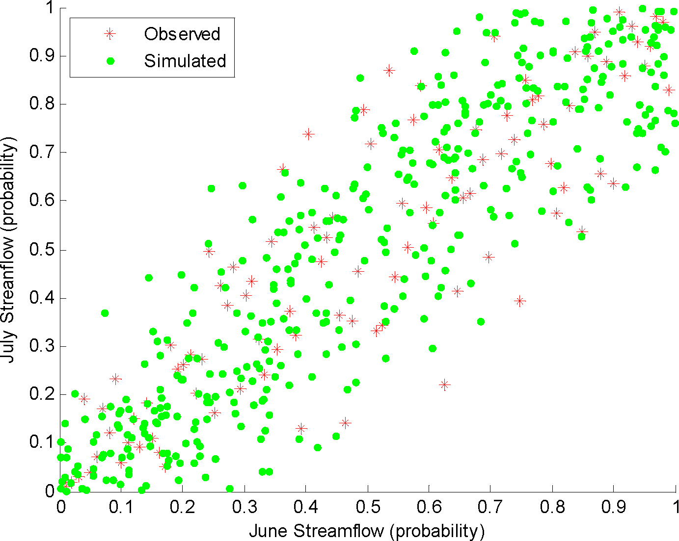
Monthly streamflow from the Colorado River basin from 1906 to 2003 [107] is used in this study to assess the performance of the entropy copula for the hydrologic simulation. For simplicity, monthly streamflow of June and July of the station at Lees Ferry, Arizona on the Colorado River is used to illustrate the application. The scatterplot of June and July monthly streamflows is shown in Figure 1. Since strong dependence of stremaflow of the two months is revealed from Figure 1, statistical modeling of the joint behavior in applications, such as streamflow simulation, requires suitable characterizations of the dependence structure.

Following [22], the first three moments of marginal probabilities of June and July monthly streamflow are used as constraints. In addition, for the dependence structure between monthly streamflow of the two months, the Spearman rank correlation is used as a dependence measure here. Moreover, the Blest measure [108,109] is used as another dependence measure to illustrate the flexibility of entropy copula for dependence modeling. The Blest measure type I (b) is expressed as:

$$b=2-12{\displaystyle {\int }_0^1}{\displaystyle {\int }_0^1}{(1-u)}^{2}vc(u,v)dudv$$

(53)

The Blest measure can be modeled by specifying g(u,v) = (1−u)²v in Equation (21). Based on Equation (29), the maximum entropy copula of monthly streamflows of June (u) and July (v) can be obtained as:

$$c(u,v)=\frac{\exp \left[-{\lambda }_0-{\displaystyle \sum _{r=1}^3\left({\lambda }_r{u}^r+{\lambda }_{r+3}{v}^r\right)-{\lambda }_{7}uv-{\lambda }_8{(1-u)}^{2}v}\right]}{{\displaystyle {\int }_0^1{\displaystyle {\int }_0^1\exp \left[-{\displaystyle \sum _{r=1}^3\left({\lambda }_r{u}^r+{\lambda }_{r+3}{v}^r\right)-{\lambda }_{7}uv-{\lambda }_8{(1-u)}^{2}v)}\right]}}dudv}$$

(54)

where λ₁, …, λ₆ are associated with the constraints with respect to marginal properties, λ₇ and λ₈ are associated with the Spearman rank correlation and Blest measure, respectively. In total one has 8 Lagrange multiplier or parameters to be estimated, which can be achieved by the Newton-Raphson method [22,55]. Based on the bivariate copula, the conditional distribution of monthly streamflow of a specific month conditioned on streamflow of another month can be constructed for simulations.

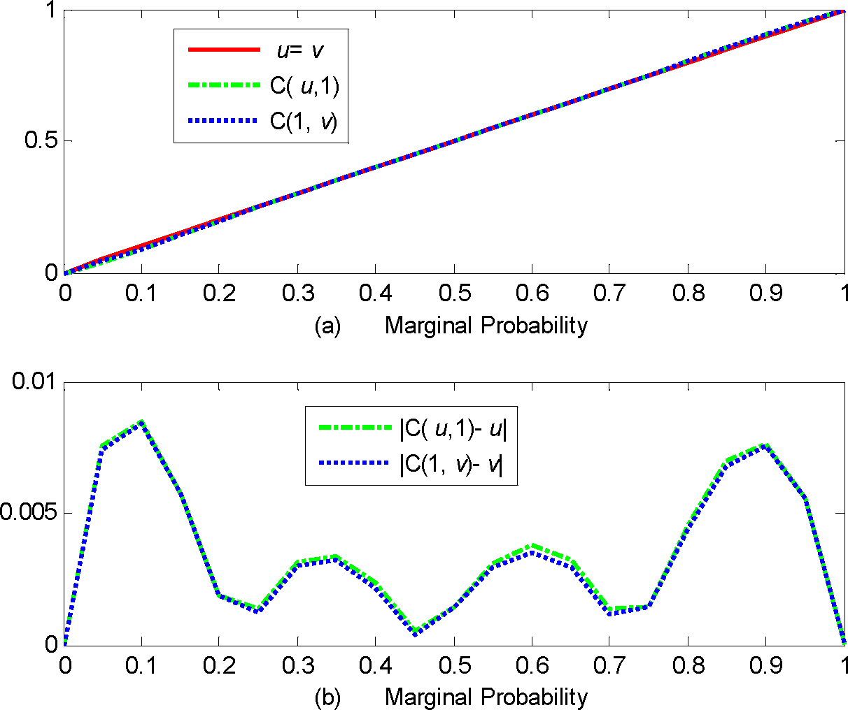
Following [17], the marginal probability distributions of the entropy copula are first validated, as shown in Figure 2a. The absolute difference between the theoretical and approximated marginal probability is shown in Figure 2b. Generally the theoretical marginal probability matches the empirical probability relatively well (with the absolute bias smaller than 10⁻²).

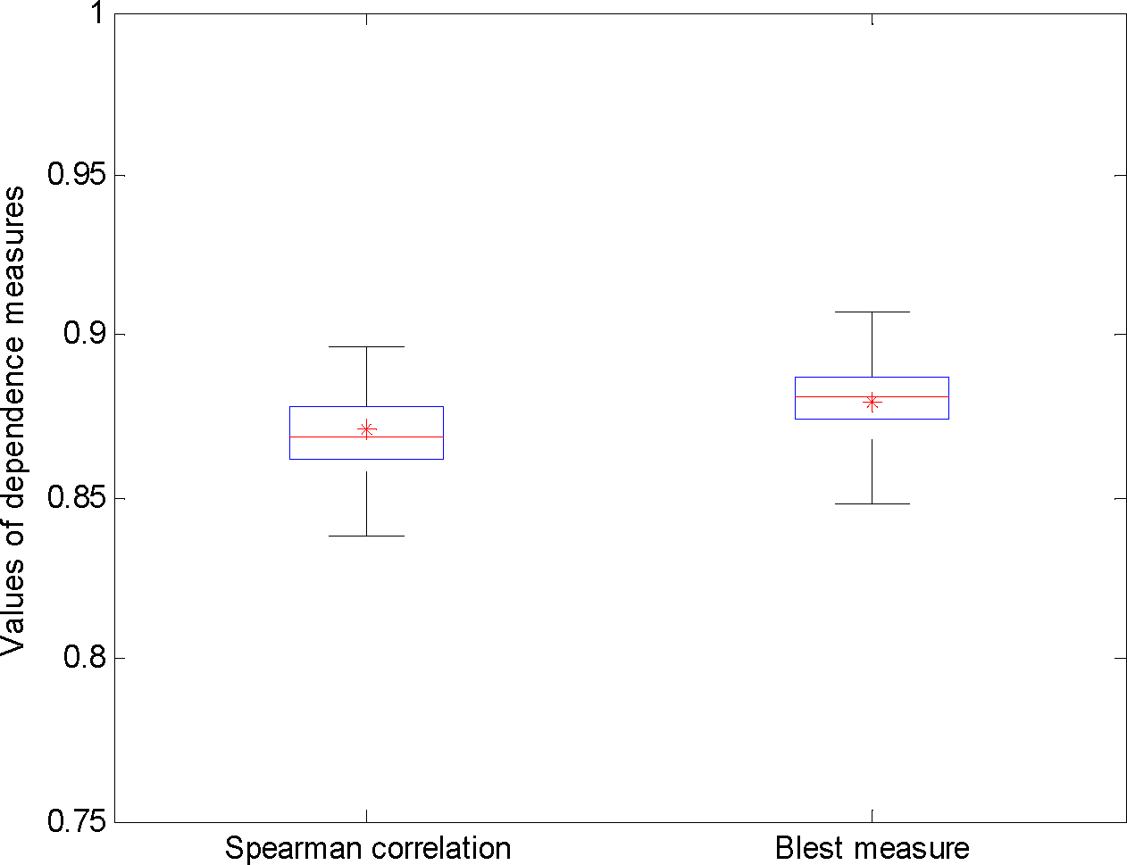
The performance of entropy copula in modeling the dependence of monthly streamflow is then assessed. First, one sequence of the random vectors of the June and July streamflow probabilities is shown in Figure 1. It can be seen that the spread of the simulated streamflow matches that of the observed streamflow quite well. In addition, the Spearman correlation of the simulated random vectors is 0.85, which is close to that of the observations (0.87). To show the performance of this model, 100 flow sequences (400 random vectors for each sequence) are generated from the entropy copula model. The boxplot of the simulated spearman correlation and Blest measure of the flow sequences is shown in Figure 3, for which the central mark of the box is the median and the end lines of the box represent 25th and 75th percentiles. It is shown that the observed Spearman and Blest dependences fall within the boxplot, implying that the dependence structure of the observed June and July streamflow pairs can be simulated relatively well.

5.2. Copula Entropy for Dependence Analysis

Climate change has altered not only the overall magnitude of hydro-climatic variables but also the seasonal distribution and inter-annual variability [110], including extremes [111]. A variety of studies have confirmed the climate change impacts on the intensity and frequency of precipitation and temperature [112], such as increasing trends in extreme events, including floods, droughts, and heatwaves due to the warming climate [113–115]. Variations in precipitation and temperature are closely associated due to their thermodynamic relations [116] and observed changes in regional temperature and precipitation can often be physically related to one another [117]. Past studies have explored the relationship and co-variability of precipitation and temperature in different seasons and regions [116–119], for which statistical distributions have been commonly used to explore their joint behavior [120–124]. The covariability of precipitation and temperature may result in the occurrence of joint climate extremes, such as drought and heatwave, which may amplify the impact of the individual extreme [125–127]. Recently, studies on the changes of joint occurrence of precipitation and temperature extremes have attracted much attention [123,128–130]. However, impacts of climate change on the dependence structure of precipitation and temperature (or other variables) have seldom been assessed. In this section, the mutual information, in terms of copula entropy, is used as a measure of nonlinear dependence to assess potential impacts of climate change on the dependence structure of precipitation and temperature.

Daily precipitation and temperature for the station at Dallas Fort Worth, TX for the period 1948–2010 is used for this application, which can be obtained from the Global Historical Climatology Network (GHCN) version 2 data. Annual mean temperature and precipitation are then compiled from daily data for the same period. The period 1948–1980 is selected as the baseline period and the future periods after the baseline period for every five years (e.g., 1948–1985, 1948–1990, …, 1948–2010) are selected to assess the changes. For each period, the copula-based joint distribution can be estimated to compute the copula entropy for dependence analysis. For simplicity, the Gaussian copula is used to model the joint distribution of precipitation and temperature for each period, which is then used to compute the copula entropy.

The general equation to compute the mutual information or copula entropy is shown in Equation (48). As introduced previously, the multiple integration method and Monte Carlo method can be used for the estimation of copula entropy. For the Gaussian copula with the correlation coefficient ρ, the analytical expression of the copula entropy is available, which can be expressed as [16]:

$$MI=-\frac{1}{2}\log (1-{\rho }^2)$$

(55)

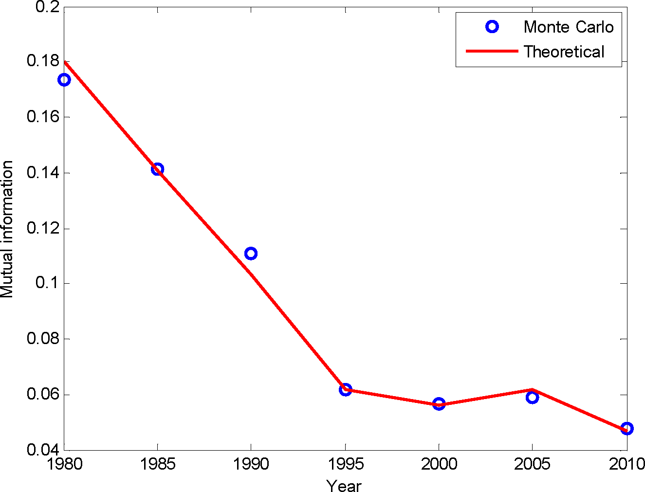
The mutual information based on the Gaussian copula computed from Equation (55) for different periods up to 2010 is shown in Figure 4. The month Carlo simulation is also used to compute the copula entropy and is shown in Figure 4, which matches the theoretical values well. From Figure 4, it is observed that mutual information has been decreasing for the past half century. For example, the mutual information for the period 1948–1980 is 0.18, which decreases to 0.06 for the period 1948–2005. The decrease of mutual information is likely to result from the climate change, implying that the climate change may impact the dependence structure of precipitation and temperature of this station. However, it is recognized that other factors may affect the decreasing pattern of the mutual information in Figure 4, such as data length and the copula family used for the computation.

6. Discussion

The entropy copula provides an alternative way to derive the copula function. When there is no prior information about the copula, the one with the maximum entropy subject to certain constraints can be selected to construct the joint distribution for dependence modeling. The entropy copula is essentially a copula family and shares attractive properties with the commonly used copulas, such as the modeling of dependence structures independent of the modeling of marginal probability distributions. The unique feature of the entropy copula in the dependence modeling is that the dependence of particular interest can be modeled by specifying associated constraints, which would be a useful complement to the current research efforts in dependence modeling. Thus, as a copula family in its own right, it can be employed in a variety of applications, such as frequency analysis, rainfall simulation, geo-statistical interpolation, rainfall (and streamflow) simulation and disaggregation, weather generator, bias correction, statistical downscaling, uncertainty analysis, statistical forecasting, to name but a few, where the dependence modeling is involved [22]. Due to its flexibility in modeling various dependence structures, it is expected that the entropy copula would be an attractive tool in the modeling of temporal and spatial dependence structure in various applications in hydrology and water resources.

Though it is straightforward to extend the entropy copula for modeling dependence in high dimensions, the potential drawbacks would be the computational burden due to relatively large number of Lagrange multipliers (or parameters) associated with marginals and dependence structures. The recently developed vine copula (or pair copula construction) with flexible dependence modeling in higher dimensions may be an attractive alternative in this case [86,131–133]. In addition, since the marginal probability is approximated with biases, much attention has to be paid for certain applications, especially when the extrapolation is needed. For example, based on the absolute bias of the marginal probability in Section 5.1, the fitted entropy copula is not appropriate for frequency analysis of rare (extreme) events associated with low probabilities (e.g., exceedance probability 0.005 or return period 200 years), for which the extrapolation in the tail region is of particular interest.

As an entropy-based copula family, the entropy copula is related to other commonly used copula families. With the suitable specification of marginal probabilities and dependence structures, the Gaussian copula can be derived with the principle of maximum entropy [29]. The entropy copula can also be interpreted as the approximation of the copula, for which other types of copula approximation schemes exist [95,97,134,135], such as shuffle of min copula[136,137], Bernstein copula [138,139], checkerboard copula [31,134] or others based on splines or kernels[140–142]. Moreover, the entropy based bivariate copula can also be integrated in the vine structure to derive the vine copula [32], which is particularly attractive in modeling the flexible dependence in higher dimensions when parametric copulas fall short in this case [88,132].

Dependence measures, such as linear correlation, rank correlation, and tail dependence, play an important role in evaluating/assessing the model performance, predictability, network design, or climate change. The mutual information (copula entropy) provides a measure of all-order (nonlinear) dependence, which is an important alternative to commonly used dependence measures, such as linear correlation. Moreover, most of the commonly used dependence measures are only applicable in the bivariate case and would fall short in dependence measures of multiple variables. The copula entropy, which is shown to be the negative total correlation (or multivariate mutual information), would serve as an attractive dependence measure in high dimensions.

7. Conclusions

Entropy theory has been used in a variety of applications, including probability inference, while the copula has motivated a flurry of applications for multivariate distribution constructions in the past few decades. The integration of entropy and copula theories has been recently explored in hydrology, which provides new insights in hydrologic dependence modeling and analysis. This paper introduces two branches of the articulation of the two theories in dependence modeling and analysis in hydrology and water resources with two case studies to illustrate their applications.

The entropy copula provides an alternative in the statistical inference of multivariate distributions for dependence modeling in hydrology by specifying desired properties of marginals and dependence structures as constraints. The case study of streamflow simulation illustrates the application of entropy copula in modeling the dependence of monthly streamflows, for which the Spearman correlation and Blest measure can be preserved well. Due to its flexibility of dependence modeling, it is expected that entropy copula would provide useful alternatives in dependence modeling for hydrological applications, including frequency analysis, rainfall simulation, geo-statistical interpolation, bias correction, downscaling, statistical forecast, and uncertainty analysis. The potential drawbacks in the entropy copula applications would be the computational burden due to the large number of Lagrange multipliers (or parameters) and the error resulting from approximating marginal probability distributions. The copula entropy, which is shown to be the negative mutual information (or total correlation), provides an alternative measure of dependence. The advantage of the copula entropy resides in its nonlinear dependence measure even for higher dimensions. The case study of assessing climate change impacts on the dependence structure of precipitation and temperature demonstrates the application of copula entropy in the dependence analysis. Overall, the integration of entropy and copula concepts provides useful insights in the dependence modeling and analysis in hydrology and is expected to be explored in the future to aid water resources planning and management. The original code for the entropy copula and copula entropy can be obtained from the authors upon request.

References

- Hao, Z.; Singh, V.P. Entropy-based method for bivariate drought analysis. J. Hydrol. Eng. 2013, 18, 780–786. [Google Scholar]
- Favre, A.C.; El Adlouni, S.; Perreault, L.; Thiémonge, N.; Bobée, B. Multivariate hydrological frequency analysis using copulas. Water Resour. Res. 2004, 40. doi: 01110.01029/02003WR002456. [Google Scholar]
- Zhang, L.; Singh, V.P. Bivariate rainfall frequency distributions using archimedean copulas. J. Hydrol. 2007, 332, 93–109. [Google Scholar]
- Zhang, L.; Singh, V.P. Trivariate flood frequency analysis using the gumbel-hougaard copula. J. Hydrol. Eng. 2007, 12, 431–439. [Google Scholar]
- Yue, S.; Ouarda, T.; Bobée, B.; Legendre, P.; Bruneau, P. The gumbel mixed model for flood frequency analysis. J. Hydrol. 1999, 226, 88–100. [Google Scholar]
- Singh, V.P. Entropy Theory and Its Application in Environmental and Water Engineering; Wiley: New York, NY, USA, 2013. [Google Scholar]
- Genest, C.; Favre, A.-C. Everything you always wanted to know about copula modeling but were afraid to ask. J. Hydrol. Eng. 2007, 12, 347–368. [Google Scholar]
- Singh, V.P. Hydrologic synthesis using entropy theory: Review. J. Hydrol. Eng. 2011, 16, 421–433. [Google Scholar]
- Singh, V.P. The use of entropy in hydrology and water resources. Hydrol. Process. 1997, 11, 587–626. [Google Scholar]
- Singh, V.P. Introduction to Entropy Theory in Hydrologic Science and Engineering; McGraw-Hill Education: New York, NY, USA, 2015. [Google Scholar]
- Nelsen, R.B. An Introduction to Copulas; Springer: New York, NY, USA, 2006. [Google Scholar]
- Schoelzel, C.; Friederichs, P. Multivariate non-normally distributed random variables in climate research–introduction to the copula approach. Nonlinear Process. Geophys. 2008, 15, 761–772. [Google Scholar]
- Genest, C.; Nešlehová, J. Copula Modeling for Extremes. In Encyclopedia of Environmetrics, 2nd ed.; El-Shaarawi, A.H., Piegorsch, W.W., Eds.; Wiley: Chichester, UK, 2012; Volume 2, pp. 530–541. [Google Scholar]
- Salvadori, G.; De Michele, C. On the use of copulas in hydrology: Theory and practice. J. Hydrol. Eng. 2007, 12, 369–380. [Google Scholar]
- Hao, Z.; Singh, V.P. Drought characterization from a multivariate perspective: A review. J. Hydrol. 2015. submitted. [Google Scholar]
- Calsaverini, R.S.V.R. An information-theoretic approach to statistical dependence: Copula information. Europhys. Lett. 2009, 88, 68003. [Google Scholar]
- Chu, B. Recovering copulas from limited information and an application to asset allocation. J. Bank. Financ. 2011, 35, 1824–1842. [Google Scholar]
- Bedford, T.; Wilson, K.J. On the construction of minimum information bivariate copula families. Ann. Inst. Stat. Math. 2014, 66, 703–723. [Google Scholar]
- Hao, Z.; Singh, V.P. Entropy-copula method for single-site monthly streamflow simulation. Water Resour. Res. 2012, 48, W06604. [Google Scholar]
- Hao, Z. Application of Entropy Theory in Hydrologic Analysis and Simulation. Ph.D Thesis, Texas A&M University, College Station, TX, USA, 2012. [Google Scholar]
- Borwein, J.; Howlett, P.; Piantadosi, J. Modelling and simulation of seasonal rainfall using the principle of maximum entropy. Entropy 2014, 16, 747–769. [Google Scholar]
- Hao, Z.; Singh, V.P. Modeling multi-site streamflow dependence with maximum entropy copula. Water Resour. Res. 2013, 49. [Google Scholar] [CrossRef]
- Kong, X.; Huang, G.; Fan, Y.; Li, Y. Maximum entropy-gumbel-hougaard copula method for simulation of monthly streamflow in Xiangxi River, China. Stoch. Env. Res. Risk Assess 2014, 29, 833–846. [Google Scholar]
- Zachariah, M.; Reddy, M.J. Development of an entropy-copula-based stochastic simulation model for generation of monthly inflows into the Hirakud Dam. ISH J. Hyd. Eng. 2013, 19, 267–275. [Google Scholar]
- Singh, V.P. Entropy-Based Parameter Estimation in Hydrology; Kluwer Academic Publishers: Dordrecht, The Netherlands, 1998. [Google Scholar]
- Kapur, J. Maximum-Entropy Models in Science and Engineering; Wiley: New York, NY, USA, 1989. [Google Scholar]
- Frank, S.A.; Smith, E. A simple derivation and classification of common probability distributions based on information symmetry and measurement scale. J. Evol. Biol. 2010, 469–484. [Google Scholar]
- Chui, C.; Wu, X. Exponential series estimation of empirical copulas with application to financial returns. Adv. Econ. 2009, 25, 263–290. [Google Scholar]
- Pougaza, D.B.; Mohammad-Djafari, A.; Bercher, J.F. Link between copula and tomography. Pattern Recogn. Lett. 2010, 31, 2258–2264. [Google Scholar] [Green Version]
- Piantadosi, J.; Howlett, P.; Boland, J. Matching the grade correlation coefficient using a copula with maximum disorder. J. Ind. Manag. Optim. 2007, 3, 305–312. [Google Scholar]
- Piantadosi, J.; Howlett, P.; Borwein, J. Copulas with maximum entropy. Optim. Lett. 2012, 6, 99–125. [Google Scholar]
- Meeuwissen, A.; Bedford, T. Minimally informative distributions with given rank correlation for use in uncertainty analysis. J. Stat. Comput. Sim. 1997, 57, 143–174. [Google Scholar]
- Dempster, M.A.H.; Medova, E.A.; Yang, S.W. Empirical copulas for cdo tranche pricing using relative entropy. Int. J. Theor. Appl. Financ. 2007, 10, 679–701. [Google Scholar]
- Hao, Z.; Singh, V.P. Single-site monthly streamflow simulation using entropy theory. Water Resour. Res. 2011, 47, W09528, doi: 09510.01029/02010WR010208. [Google Scholar]
- Ma, J.; Sun, Z. Mutual information is copula entropy. Tsinghua Sci. Technol. 2011, 16, 51–54. [Google Scholar]
- Alfonso, L.; Lobbrecht, A.; Price, R. Information theory–based approach for location of monitoring water level gauges in polders. Water Resour. Res. 2010, 46. [Google Scholar] [CrossRef]
- Papalexiou, S.M.; Koutsoyiannis, D. Entropy based derivation of probability distributions: A case study to daily rainfall. Adv. Water Resour 2012, 45, 51–57. [Google Scholar]
- Hao, Z.; Singh, V.P. Entropy-based method for extreme rainfall analysis in texas. J. Geophys. Res.-Atmos. 2013, 118, 263–273. [Google Scholar]
- Hao, Z.; Singh, V.P. Entropy-based parameter estimation for extended burr xii distribution. Stoch. Env. Res. Risk Assess 2009, 23, 1113–1122. [Google Scholar]
- Woodbury, A.; Ulrych, T. Minimum relative entropy: Forward probabilistic modeling. Water Resour. Res. 1993, 29, 2847–2860. [Google Scholar]
- Hou, Z.; Rubin, Y. On minimum relative entropy concepts and prior compatibility issues in vadose zone inverse and forward modeling. Water Resour. Res. 2005, 41, W12425. [Google Scholar]
- Woodbury, A.; Ulrych, T. Minimum relative entropy inversion: Theory and application to recovering the release history of a groundwater contaminant. Water Resour. Res. 1996, 32, 2671–2681. [Google Scholar]
- Mishra, A.K.; Özger, M.; Singh, V.P. An entropy-based investigation into the variability of precipitation. J. Hydrol. 2009, 370, 139–154. [Google Scholar]
- Mishra, A.K.; Özger, M.; Singh, V.P. Association between uncertainties in meteorological variables and water-resources planning for the state of texas. J. Hydrol. Eng. 2010, 16, 984–999. [Google Scholar]
- Rajsekhar, D.; Mishra, A.K.; Singh, V.P. Regionalization of drought characteristics using an entropy approach. J. Hydrol. Eng. 2012, 18, 870–887. [Google Scholar]
- Li, C.; Singh, V.P.; Mishra, A.K. Entropy theory-based criterion for hydrometric network evaluation and design: Maximum information minimum redundancy. Water Resour. Res. 2012, 48. [Google Scholar] [CrossRef]
- Mishra, A.K.; Coulibaly, P. Variability in canadian seasonal streamflow information and its implication for hydrometric network design. J. Hydrol. Eng. 2014, 19, 05014003. [Google Scholar]
- Mishra, A.; Coulibaly, P. Hydrometric network evaluation for canadian watersheds. J. Hydrol. 2010, 380, 420–437. [Google Scholar]
- Shannon, C.E. A mathematical theory of communications. Bell Syst. Tech. J 1948, 27, 379–423. [Google Scholar]
- Shannon, C.; Weaver, W. The Mathematical Theory of Communication; University Illinois Press: Champaign, IL, USA, 1949. [Google Scholar]
- Singh, V.P. Entropy Theory in Hydraulic Engineering: An Introduction; ASCE Press: Reston, VA, USA, 2014. [Google Scholar]
- Jaynes, E.T. Information theory and statistical mechanics. Phys. Rev. 1957, 106, 620–630. [Google Scholar]
- Jaynes, E.T. Information theory and statistical mechanics. II. Phys. Rev. 1957, 108, 171–190. [Google Scholar]
- Kesavan, H.; Kapur, J. Entropy Optimization Principles with Applications; Academic Press: New York, NY, USA, 1992. [Google Scholar]
- Mead, L.; Papanicolaou, N. Maximum entropy in the problem of moments. J. Math. Phys. 1984, 25, 2404–2417. [Google Scholar]
- Cover, T.; Thomas, J. Elementary of Information Theory; Wiley: New York, NY, USA, 1991. [Google Scholar]
- Dirmeyer, P.A.; Wei, J.; Bosilovich, M.G.; Mocko, D.M. Comparing evaporative sources of terrestrial precipitation and their extremes in merra using relative entropy. J. Hydrometeorol. 2014, 15, 102–116. [Google Scholar]
- Kleeman, R. Measuring dynamical prediction utility using relative entropy. J. Atmos. Sci. 2002, 59, 2057–2072. [Google Scholar]
- Brunsell, N. A multiscale information theory approach to assess spatial–temporal variability of daily precipitation. J. Hydrol. 2010, 385, 165–172. [Google Scholar]
- Majda, A.; Kleeman, R.; Cai, D. A mathematical framework for quantifying predictability through relative entropy. Methods Appl. Anal. 2002, 9, 425–444. [Google Scholar]
- DelSole, T.; Tippett, M.K. Predictability: Recent insights from information theory. Rev. Geophys. 2007, 45. [Google Scholar] [CrossRef]
- DelSole, T. Predictability and information theory. Part II: Imperfect forecasts. J. Atmos. Sci. 2005, 62, 3368–3381. [Google Scholar]
- DelSole, T. Predictability and information theory. Part I: Measures of predictability. J. Atmos. Sci. 2004, 61, 2425–2440. [Google Scholar]
- Feng, X.; Porporato, A.; Rodriguez-Iturbe, I. Changes in rainfall seasonality in the tropics. Nat. Clim. Chang. 2013, 3, 811–815. [Google Scholar]
- Pascale, S.; Lucarini, V.; Feng, X.; Porporato, A. Projected changes of rainfall seasonality and dry spells in a high concentration pathway 21st century scenario arXiv preprint. 2014, arXiv, 1410.3116.
- Kullback, S.; Leibler, R. On information and sufficiency. Ann. Math. Stat. 1951, 22, 79–86. [Google Scholar]
- Kullback, S. Statistics and Information Theory; Wiley: New York, NY, USA, 1959. [Google Scholar]
- Salvadori, G.; de Michele, C. Multivariate multiparameter extreme value models and return periods: A copula approach. Water Resour. Res. 2010, 46. [Google Scholar] [CrossRef]
- Khedun, C.P.; Chowdhary, H.; Mishra, A.K.; Giardino, J.R.; Singh, V.P. Water deficit duration and severity analysis based on runoff derived from noah land surface model. J. Hydrol. Eng. 2012, 18, 817–833. [Google Scholar]
- Bardossy, A.; Li, J. Geostatistical interpolation using copulas. Water Resour. Res. 2008, 44, W07412, doi: 07410.01029/02007WR006115. [Google Scholar]
- Piani, C.; Haerter, J. Two dimensional bias correction of temperature and precipitation copulas in climate models. Geophys. Res. Lett. 2012, 39. [Google Scholar] [CrossRef]
- Chowdhary, H.; Singh, V.P. Reducing uncertainty in estimates of frequency distribution parameters using composite likelihood approach and copula-based bivariate distributions. Water Resour. Res. 2010, 46, W11516. [Google Scholar] [CrossRef]
- Laux, P.; Vogl, S.; Qiu, W.; Knoche, H.; Kunstmann, H. Copula-based statistical refinement of precipitation in rcm simulations over complex terrain. Hydrol. Earth Syst. Sci. 2011, 15, 2401–2419. [Google Scholar]
- Khedun, C.P.; Mishra, A.K.; Singh, V.P.; Giardino, J.R. A copula-based precipitation forecasting model: Investigating the interdecadal modulation of enso’s impacts on monthly precipitation. Water Resour. Res. 2014, 50, 580–600. [Google Scholar]
- Jaworski, P.; Durante, F.; Härdle, W.K.; Rychlik, T. Copula Theory and its Applications. In Lecture Notes in Statistics—Proceedings; Springer: New York, NY, USA, 2010. [Google Scholar]
- Patton, A.J. A review of copula models for economic time series. J. Multivar. Anal. 2012, 110, 4–18. [Google Scholar]
- Genest, C.; Nešlehová, J. Copulas and Copula Models. In Encyclopedia of Environmetrics, 2nd ed.; El-Shaarawi, A.H., Piegorsch, W.W., Eds.; Wiley: Chichester, UK, 2012; Volume 2, pp. 541–553. [Google Scholar]
- Joe, H. Multivariate Models and Dependence Concepts; Chapman & Hall: London, UK, 1997. [Google Scholar]
- Genest, C.; Favre, A.C.; Béliveau, J.; Jacques, C. Metaelliptical copulas and their use in frequency analysis of multivariate hydrological data. Water Resour. Res. 2007, 43, W09401, doi: 09410.01029/02006WR005275. [Google Scholar]
- Song, S.; Singh, V.P. Meta-elliptical copulas for drought frequency analysis of periodic hydrologic data. Stoch. Env. Res. Risk Assess 2010, 24, 425–444. [Google Scholar]
- Singh, V.; Zhang, L. Idf curves using the frank archimedean copula. J. Hydrol. Eng. 2007, 12, 651–662. [Google Scholar]
- Kao, S.C.; Govindaraju, R.S. Trivariate statistical analysis of extreme rainfall events via the plackett family of copulas. Water Resour. Res. 2008, 44, W02415, doi: 02410.01029/02007WR006261. [Google Scholar]
- Song, S.; Singh, V. Frequency analysis of droughts using the plackett copula and parameter estimation by genetic algorithm. Stoch. Env. Res. Risk Assess 2010, 24, 783–805. [Google Scholar]
- Salvadori, G.; de Michele, C.; Kottegoda, N.; Rosso, R. Extremes in Nature: An Approach Using Copulas; Springer: New York, NY, USA, 2007; Volume 1. [Google Scholar]
- Kurowicka, D.; Joe, H. Dependence Modeling: Vine Copula Handbook; World Scientific: Singapore, 2011. [Google Scholar]
- Bedford, T.; Cooke, R.M. Probability density decomposition for conditionally dependent random variables modeled by vines. Ann. Math. Artif. Intel. 2001, 32, 245–268. [Google Scholar]
- Gyasi-Agyei, Y. Copula-based daily rainfall disaggregation model. Water Resour. Res. 2011, 47, W07535. [Google Scholar] [CrossRef]
- Joe, H.; Li, H.; Nikoloulopoulos, A.K. Tail dependence functions and vine copulas. J. Multivar. Anal. 2010, 101, 252–270. [Google Scholar]
- Aas, K.; Czado, C.; Frigessi, A.; Bakken, H. Pair-copula constructions of multiple dependence. Insur. Math. Econ. 2009, 44, 182–198. [Google Scholar]
- Genest, C.; Ghoudi, K.; Rivest, L.-P. A semiparametric estimation procedure of dependence parameters in multivariate families of distributions. Biometrika 1995, 82, 543–552. [Google Scholar]
- Genest, C.; Carabarín-Aguirre, A.; Harvey, F. Copula parameter estimation using blomqvist’s beta. J. Soc. Fr. Stat. 2013, 154, 5–24. [Google Scholar]
- MATLAB function ADAPT. Available online: http://www.math.wsu.edu/math/faculty/genz/homepage accessed on 10 March 2015.
- Mayor, G.; Suñer, J.; Torrens, J. Copula-like operations on finite settings. IEEE Trans. Fuzzy Syst 2005, 13, 468–477. [Google Scholar]
- Kolesárová, A.; Mesiar, R.; Mordelová, J.; Sempi, C. Discrete copulas. IEEE Trans. Fuzzy Syst 2006, 14, 698–705. [Google Scholar]
- Li, X.; Mikusiński, P.; Taylor, M.D. Strong approximation of copulas. J. Math. Anal. Appl. 1998, 225, 608–623. [Google Scholar]
- Piantadosi, J.; Howlett, P.; Borwein, J.; Henstridge, J. Maximum entropy methods for generating simulated rainfall. Numer. Algebra. Contr. Optim. 2012, 2, 233–256. [Google Scholar]
- Li, X.; Mikusiński, P.; Sherwood, H.; Taylor, M.D. On approximation of copulas. In Distributions with Given Marginals and Moment Problems; Beneš, V., Štěpán, J., Eds.; Springer: Dordrecht, The Netherlands, 1997; pp. 107–116. [Google Scholar]
- Lanford, O.E. Entropy and Equilibrium States in Classical Statistical Mechanics. In Statistical Mechanics and Mathematical Problems; Lenard, A., Ed.; Springer: New York, NY, USA, 1973; pp. 1–113. [Google Scholar]
- Borwein, J.M.; Lewis, A.S. Convex Analysis and Nonlinear Optimization: Theory and Examples; Springer: New York, NY, USA, 2010. [Google Scholar]
- Centre for Computer Assisted Research Mathematics and its Applications (CARMA) website. Available online: http://docserver.carma.newcastle.edu.au/1453/1/ecr.pdf accessed on 10 March 2015.
- Kraskov, A.; Stögbauer, H.; Grassberger, P. Estimating mutual information. Phys. Rev. E 2004, 69, 066138. [Google Scholar]
- Joe, H. Relative entropy measures of multivariate dependence. J. Am. Stat. Assoc. 1989, 84, 157–164. [Google Scholar]
- Chow, C.; Liu, C. Approximating discrete probability distributions with dependence trees. IEEE Trans. Inf. Theory. 1968, 14, 462–467. [Google Scholar]
- McGill, W.J. Multivariate information transmission. Psychometrika 1954, 19, 97–116. [Google Scholar]
- Watanabe, S. Information theoretical analysis of multivariate correlation. IBM J. Res. Dev. 1960, 4, 66–82. [Google Scholar]
- Fass, D. Human Sensitivity to Mutual Information; The State University of New Jersey: New Brunswcks, NJ, USA, 2007. [Google Scholar]
- Lee, T.; Salas, J.D. Record Extension of Monthly Flows for the Colorado River System; U.S. Bureau of Reclamation, U.S. Department of the Interior: Denver, CO, USA, 2006. Available online: www.usbr.gov/lc/region/g4000/NaturalFlow/Final.RecordExtensionReport.2006.pdf accessed on 13 April 2015.
- Blest, D.C. Rank correlation—An alternative measure. Aust. N. Z. J. Stat. 2000, 42, 101–111. [Google Scholar]
- Genest, C.; Plante, J.F. On blest’s measure of rank correlation. Can. J. Stat. 2003, 31, 35–52. [Google Scholar]
- Stocker, T.F.; Qin, D.; Plattner, G.-K.; Tignor, M.M.B.; Allen, S.K.; Boschung, J.; Nauels, A.; Xia, Y.; Bex, V.; Midgley, P.M. (Eds.) Climate Change 2013: The Physical Science Basis. Contribution of Working Group I to the Fifth Assessment Report of the Intergovernmental Panel on Climate Change; Cambridge University Press: New York, NY, USA, 2013.
- Easterling, D.R.; Evans, J.; Groisman, P.Y.; Karl, T.; Kunkel, K.E.; Ambenje, P. Observed variability and trends in extreme climate events: A brief review. Bull. Am. Meteor. Soc. 2000, 81, 417–425. [Google Scholar]
- Katz, R.W. Statistics of extremes in climate change. Clim. Chang. 2010, 100, 71–76. [Google Scholar]
- Rahmstorf, S.; Coumou, D. Increase of extreme events in a warming world. Proc. Natl. Acad. Sci. USA 2011, 108, 17905–17909. [Google Scholar]
- Coumou, D.; Rahmstorf, S. A decade of weather extremes. Nat. Clim. Chang. 2012, 2, 491–496. [Google Scholar]
- Rummukainen, M. Changes in climate and weather extremes in the 21st century. Wiley Interdiscip. Rev. 2012, 3, 115–129. [Google Scholar]
- Adler, R.F.; Gu, G.; Wang, J.J.; Huffman, G.J.; Curtis, S.; Bolvin, D. Relationships between global precipitation and surface temperature on interannual and longer timescales 1979–2006. J. Geophys. Res. 2008, 113, D22104. [Google Scholar]
- Solomon, S.; Qin, D.; Manning, M.; Chen, Z.; Marquis, K.B.; Averyt, M.; Tignor, M.; Miller, H.L. (Eds.) Climate Change 2007: The Physical Science Basis: Contribution of Working Group I to the Fourth Assessment Report of the Intergovernmental Panel on Climate Change; Cambridge University Press: Cambridge, UK and New York, NY, USA, 2007; Volume 4.
- Liu, C.; Allan, R.P.; Huffman, G.J. Co-variation of temperature and precipitation in cmip5 models and satellite observations. Geophys. Res. Lett. 2012, 39, L13803. [Google Scholar]
- Trenberth, K.E.; Shea, D.J. Relationships between precipitation and surface temperature. Geophys. Res. Lett. 2005, 32, L14703. [Google Scholar]
- Tebaldi, C.; Sansó, B. Joint projections of temperature and precipitation change from multiple climate models: A hierarchical bayesian approach. J. R. Stat. Soc. A 2009, 172, 83–106. [Google Scholar]
- Sexton, D.M.H.; Murphy, J.M.; Collins, M.; Webb, M.J. Multivariate probabilistic projections using imperfect climate models part I: Outline of methodology. Clim. Dynam. 2012, 38, 2513–2542. [Google Scholar]
- Watterson, I. Calculation of joint pdfs for climate change with properties matching recent australian projections. Aust. Meteorol. Ocean. J 2011, 61, 211–219. [Google Scholar]
- Estrella, N.; Menzel, A. Recent and future climate extremes arising from changes to the bivariate distribution of temperature and precipitation in bavaria, germany. Int. J. Climatol. 2012, 33, 1687–1695. [Google Scholar]
- Rodrigo, F. On the covariability of seasonal temperature and precipitation in spain, 1956–2005. Int. J. Climatol. 2014, in press. [Google Scholar]
- Hoerling, M.; Kumar, A.; Dole, R.; Nielsen-Gammon, J.W.; Eischeid, J.; Perlwitz, J.; Quan, X.-W.; Zhang, T.; Pegion, P.; Chen, M. Anatomy of an extreme event. J. Clim. 2013, 26, 2811–2832. [Google Scholar]
- Karl, T.; Gleason, B.; Menne, M.; McMahon, J.; Heim, R.; Brewer, M.; Kunkel, K.; Arndt, D.; Privette, J.; Bates, J. Us temperature and drought: Recent anomalies and trends. Eos Trans Am. Geophys. Union. 2012, 93, 473–474. [Google Scholar]
- Lyon, B.; Dole, R.M. A diagnostic comparison of the 1980 and 1988 US summer heat wave-droughts. J. Clim. 1995, 8, 1658–1675. [Google Scholar]
- Zhang, X.; Vincent, L.A.; Hogg, W.; Niitsoo, A. Temperature and precipitation trends in Canada during the 20th century. Atmos. Ocean. 2000, 38, 395–429. [Google Scholar]
- Beniston, M. Trends in joint quantiles of temperature and precipitation in europe since 1901 and projected for 2100. Geophys. Res. Lett. 2009, 36, L07707. [Google Scholar]
- Hao, Z.; AghaKouchak, A.; Phillips, T.J. Changes in concurrent monthly precipitation and temperature extremes. Environ. Res. Lett. 2013, 8, 034014. [Google Scholar]
- Joe, H. Families of m-variate distributions with given margins and m (m-1)/2 bivariate dependence parameters. Lect. Notes Monogr. Ser. 1996, 28, 120–141. [Google Scholar]
- Bedford, T.; Cooke, R.M. Vines—A new graphical model for dependent random variables. Ann. Stat. 2002, 30, 1031–1068. [Google Scholar]
- Kurowicka, D.; Cooke, R.M. Uncertainty Analysis with High Dimensional Dependence Modelling; Wiley: New York, NY, USA, 2006. [Google Scholar]
- Kulpa, T. On approximation of copulas. Int. J. Math. Math. Sci. 1999, 22, 259–269. [Google Scholar]
- Zheng, Y.; Yang, J.; Huang, J.Z. Approximation of bivariate copulas by patched bivariate fréchet copulas. Insur. Math. Econ. 2011, 48, 246–256. [Google Scholar]
- Mikusinski, P.; Sherwood, H.; Taylor, M. Shuffles of min. Stochastica: Revista de Matemática Pura y Aplicada 1992, 13, 61–74. [Google Scholar]
- Durante, F.; Sarkoci, P.; Sempi, C. Shuffles of copulas. J. Math. Anal. Appl. 2009, 352, 914–921. [Google Scholar]
- Diers, D.; Eling, M.; Marek, S.D. Dependence modeling in non-life insurance using the bernstein copula. Insur. Math. Econ. 2012, 50, 430–436. [Google Scholar]
- Sancetta, A.; Satchell, S. The bernstein copula and its applications to modeling and approximations of multivariate distributions. Econom. Theory. 2004, 20, 535–562. [Google Scholar]
- Qu, L.; Yin, W. Copula density estimation by total variation penalized likelihood with linear equality constraints. Comput. Stat. Data Anal 2012, 56, 384–398. [Google Scholar]
- Shen, X.; Zhu, Y.; Song, L. Linear b-spline copulas with applications to nonparametric estimation of copulas. Comput. Stat. Data Anal 2008, 52, 3806–3819. [Google Scholar]
- Cormier, E.; Genest, C.; Nešlehová, J.G. Using b-splines for nonparametric inference on bivariate extreme-value copulas. Extremes 2014, 17, 633–659. [Google Scholar]
Figure 1.
Comparison of the observed and simulated streamflow pairs for June and July at the station at Lees Ferry, Arizona.
Figure 2.
Validation of marginal probabilities of the maximum entropy copula for the June and July streamflow at the station at Lees Ferry, Arizona. (a) Comparison of the estimated marginal probability with theoretical values (upper panel); (b) Absolute bias of the estimated marginal probabilities (lower panel).
Figure 3.
Comparison of observed and simulated dependence measures including Spearman rank correlation and Blest measure of the June and July streamflow pairs at the station at Lees Ferry, Arizona.
Figure 4.
Mutual information of the temperature and precipitation for the station at Dallas Fort Worth, TX.
© 2015 by the authors; licensee MDPI, Basel, Switzerland This article is an open access article distributed under the terms and conditions of the Creative Commons Attribution license (http://creativecommons.org/licenses/by/4.0/).
Share and Cite
MDPI and ACS Style
Hao, Z.; Singh, V.P. Integrating Entropy and Copula Theories for Hydrologic Modeling and Analysis. Entropy 2015, 17, 2253-2280. https://doi.org/10.3390/e17042253
AMA Style
Hao Z, Singh VP. Integrating Entropy and Copula Theories for Hydrologic Modeling and Analysis. Entropy. 2015; 17(4):2253-2280. https://doi.org/10.3390/e17042253
Chicago/Turabian StyleHao, Zengchao, and Vijay P. Singh. 2015. "Integrating Entropy and Copula Theories for Hydrologic Modeling and Analysis" Entropy 17, no. 4: 2253-2280. https://doi.org/10.3390/e17042253