On the κ-Deformed Cyclic Functions and the Generalized Fourier Series in the Framework of the κ-Algebra

Abstract

We explore two possible generalizations of the Euler formula for the complex κ-exponential, which give two different sets of κ-deformed cyclic functions endowed with different analytical properties. In a case, the κ-sine and κ-cosine functions take real values on ℜ and are characterized by an asymptotic log-periodic behavior. In the other case, the κ-cyclic functions take real values only in the region |x| ≤ 1/|κ|, while, for |x| > 1/|κ|, they assume purely imaginary values with an increasing modulus. However, the main mathematical properties of the standard cyclic functions, opportunely reformulated in the formalism of the κ-mathematics, are fulfilled by the two sets of the κ-trigonometric functions. In both cases, we study the orthogonality and the completeness relations and introduce their respective generalized Fourier series for square integrable functions.

1. Introduction

In mathematical analysis, the generalized Fourier series is a powerful tool to study the spectral decomposition of a given function over a certain orthogonal base defined on a Hilbert space. For a square integrable function f(x): [a, b] → ℜ, the generalized Fourier series is defined as:

$$f\left(x\right)=\underset{n=0}{\overset{\infty }{\Sigma }}{c}_n{u}_n\left(x\right),$$

(1)

where u_n(x) is a complete set of functions on the interval [a, b] fulfilling the orthogonality condition:

$${\langle u_n,u_m\rangle }_w=\underset{a}{\overset{b}{\int }}{u}_n\left(x\right)u_m\left(x\right)w\left(x\right)dx,$$

(2)

for a certain weight function w(x), whilst the coefficients of the series are given by:

$$c_n=\frac{{\langle f,u_n\rangle }_w}{{\langle u_n,u_n\rangle }_w}.$$

(3)

Often, the functions u_n(x) are related to a Sturm-Liouville problem for a second order differential equation:

$$\frac{d}{dx}\left(p\left(x\right)\frac{d{u}_n\left(x\right)}{dx}\right)+\left(-q\left(x\right)+\lambda w\left(x\right)\right)u_n\left(x\right)=0,$$

(4)

for given real functions p(x) and q(x) and eigenvalue λ, with suitable boundary conditions:

$$\begin{array}{cc}{a_1{u}_n\left(a\right)+a_2\frac{d{u}_n\left(x\right)}{dx}|}_{x=a}=0,& {b_1{u}_n\left(b\right)+b_2\frac{d{u}_n\left(x\right)}{dx}|}_{x=b}=0,\end{array}$$

(5)

where a_i and b_i are constants.

Depending on the nature of the problem (4), several different series expansion have been introduced in the literature, running from the trigonometric Fourier series to analyze periodic functions, to the various orthogonal polynomials expansion widely used in optic and quantum mechanics, the Bessel series for cylindrical symmetric problems, and so on.

In this paper, we propose a generalized Fourier series based on a family of orthogonal functions derived from the κ-exponential, a continuous deformation of the exponential function by means of a parameter k, that reduces to the standard exponential in the κ → 0 limit. The κ-exponential has been introduced in [1] as a possible solution of a generalized Kramer equation derived from a kinetic interaction principle. Then, the κ-exponential has been employed in statistical mechanics [2,3] to describe a formalism useful to study non-Gibbsean statistical systems characterized by power-law distributions that occur in physical and physical-like complex systems, often observed in the realm of sociophysics, econophysics, biophysics, networks and in others fields. In fact, the κ-exponential distribution is endowed by a power-law asymptotic behavior instead of the exponential shape characterizing the Gibbs distribution. It describes the equilibrium configuration of systems governed by the κ-entropy by means of the maximal entropy principle with suitable physical constraints. Up to today, several papers have been written on the foundations, the theoretical consistency and the potential applications of the κ-statistical mechanics [4–31] (see also [32] and the references therein).

As shown in [33], starting from the κ-exponential and its inverse, the κ-logarithm, it is possible to introduce a deformed mathematical structure, the κ-mathematics, equipped by a κ-algebra and the related κ-calculus. The κ-mathematics originates by requiring that the deformed exponential and logarithm preserve, as much as possible, the analytical properties of the corresponding un-deformed functions. Actually, this is a very general statement applicable to any pair of analytical functions whose shape mimics that of the exponential and of the logarithm and permits one to introduce a pair of Abelian fields, isomorphic to each other, with a generalized sum and product [34].

In the framework of the κ-mathematics, we introduce two different generalizations of the complex κ-exponential. For each of them, we obtain, by means of the Euler formula, two different sets of κ-deformed trigonometric functions that correspond to the solutions of suitable Sturm-Liouville boundary problems.

In a case, the κ-cyclic functions are obtained from the following complex κ-exponential:

$$u(x)={\exp }_{\kappa }(i\otimes x),$$

(6)

where ⊗ is the κ-product. It takes real values on ℜ and has an asymptotic log-periodic behavior. In the other case, the κ-sine and κ-cosine are obtained from the function:

$$u\left(x\right)={\exp }_{\kappa }\left(ix\right),$$

(7)

which takes real values only in the limited region |x| ≤ 1/|κ|, becoming purely imaginary and with an increasing modulus for |x| > 1/|κ|

The contents of this paper is as follows. In Section 2, we revisit the κ-algebra and the κ-calculus. In Section 3, we consider the two possible generalizations of the Euler formula in the κ-formalism and introduce the corresponding sets of cyclic-functions by studying their algebras and their analytic properties within the κ-mathematics. The orthogonality and completeness relations for the two sets of κ-cyclic functions are discussed in Section 4, while, in Section 5, we present the corresponding versions of generalized Fourier series. Our conclusions are reported in Section 6.

2. κ-Mathematics Formalism

Let us begin by revisiting the main aspects of the κ-algebra and its related calculus on which is based the formalism used in this work.

2.1. κ-Algebra

We introduce the κ-algebra starting from the κ-numbers defined in:

$$x_{\left\{\kappa \right\}}=\frac{1}{\kappa }\text{arcsinh}\left(\kappa x\right),$$

(8)

and by their dual:

$$x^{\left\{\kappa \right\}}=\frac{1}{\kappa }\text{sinh}\left(\kappa x\right),$$

(9)

with:

$${\left(x_{\left\{\kappa \right\}}\right)}^{\left\{\kappa \right\}}={\left(x^{\left\{\kappa \right\}}\right)}_{\left\{\kappa \right\}}=x.$$

(10)

The generalized sum and product are defined on the κ-numbers space ℜ^κ = {x^{κ}: −∞ < x < ∞} as follows:

$$x^{\left\{\kappa \right\}}\oplus y^{\left\{\kappa \right\}}={\left(x+y\right)}^{\left\{\kappa \right\}},$$

(11)

$$x^{\left\{\kappa \right\}}\otimes y^{\left\{\kappa \right\}}={\left(x\cdot y\right)}^{\left\{\kappa \right\}},$$

(12)

and, by replacing x^{κ} → x (and x → x_{κ}), we get:

$$x\oplus y={\left(x_{\left\{\kappa \right\}}+y_{\left\{\kappa \right\}}\right)}^{\left\{\kappa \right\}},$$

(13)

$$x\otimes y={\left(x_{\left\{\kappa \right\}}\cdot y_{\left\{\kappa \right\}}\right)}^{\left\{\kappa \right\}}.$$

(14)

They are, respectively: associative, x ⊕ (y ⊕ z) = (x ⊕ y) ⊕ z and x ⊗ (y ⊗ z) = (x ⊗ y) ⊗ z; commutative, x ⊕ y = y ⊕ x and x ⊗ y = y ⊗ x; distributed, x ⊗ (y ⊕ z) = x ⊗ y ⊕ x ⊗ z with x, y, z ∊ ℜ^κ. In addition, there exist the null element for the sum: x ⊕ Ø = Ø ⊕ x = x; and the identity for the product: x ⊗ I = I ⊗ x = x; as well as the opposite: x ⊕ (−x) = (−x) ⊕ x = Ø; and the inverse: x ⊗ (1/x) = (1/x) ⊗ x = I, for any x ∊ ℜ^κ. Therefore, the algebraic structure (ℜ^κ, ⊕, ⊗) forms an Abelian field isomorph to the field of the ordinary real numbers (ℜ, +, ·).

For the sake of completeness, let us observe that it is also possible to introduce an algebraic structure on the space of the κ-numbers ℜ_κ ≡ {x_{κ} : −∞ < x < ∞} isomorphic to (ℜ, +, ·), endowed by a generalized sum and product different from the ones given in Equations (11) and (12). We remand the interested reader to [34] for the details.

Explicitly, Equations (13) and (14) are given by:

$$x\oplus y=\frac{1}{\kappa }\text{sinh}\left(\text{arcsinh}\left(\kappa x\right)+\text{arcsinh}\left(\kappa x\right)\right),$$

(15)

$$x\otimes y=\frac{1}{\kappa }\text{sinh}\left(\frac{1}{\kappa }\text{arcsinh}\left(\kappa x\right)\cdot \text{arcsinh}\left(\kappa x\right)\right),$$

(16)

with Ø ≡ 0, I ≡ κ⁻¹ sinh κ, (−x) ≡ −x and (1/x) ≡ κ⁻¹ sinh (κ²/arcsinh κx). In this way, the difference x ⊖ y = x ⊕ (−y) and the quotient x ⊘ y = x ⊗(1/y) arise from Equations (15) and (16) as:

$$x\ominus y=\frac{1}{\kappa }\text{sinh}\left(\text{arcsinh}\left(\kappa x\right)-\text{arcsinh}\left(\kappa y\right)\right),$$

(17)

$$x\ominus y=\frac{1}{\kappa }\text{sinh}\left(\kappa \frac{\text{arcsinh}\left(\kappa x\right)}{\text{arcsinh}\left(\kappa y\right)}\right).$$

(18)

Clearly, in the κ → 0 limit, Equations (15)–(18) reduce to the standard elementary operations on the real numbers, as well as the field (ℜ^κ, ⊕, ⊗) reduces to (ℜ, +, ·).

In addition, by iteration, from the κ-sum and the κ-product, we obtain the definition of product by a κ-integer:

$$x\oplus x\oplus \dots \oplus x=n^{\left\{\kappa \right\}}\otimes x,$$

(19)

and that of power by a κ-integer:

$$x\otimes x\otimes \dots \otimes x=x^{x○\wedge n^{\left\{\kappa \right\}}}.$$

(20)

Explicitly, they are given by:

$$n^{\left\{\kappa \right\}}\otimes x=\frac{1}{\kappa }\text{sinh}\left(n\text{arcsinh}\left(\kappa x\right)\right),$$

(21)

and:

$$x^{○\wedge n^{\left\{\kappa \right\}}}=\frac{1}{\kappa }\text{sinh}\left({\kappa }^{1-n}{\text{arcsinh}}^n\left(\kappa x\right)\right).$$

(22)

In particular, this last relation can be rewritten in:

$${\left(x^{○\wedge n^{\left\{\kappa \right\}}}\right)}_{\left\{\kappa \right\}}={\left(x_{\left\{\kappa \right\}}\right)}^n,$$

(23)

and can be generalized to define the exponentiation to arbitrary real numbers:

$${\left(x^{○\wedge a}\right)}_{\left\{\kappa \right\}}={\left(x_{\left\{\kappa \right\}}\right)}^{a_{\left\{\kappa \right\}}}.$$

(24)

We introduce the κ-exponential and its inverse function, the κ-logarithm [1–3], defined in:

$${\exp }_{\kappa }x={\left(\kappa x+\sqrt{1+{\kappa }^2{x}^2}\right)}^{1/\kappa }\equiv \exp \left(\frac{1}{\kappa }\text{arcsinh}\left(\kappa x\right)\right),$$

(25)

$${\ln }_{\kappa }x=\frac{x^{\kappa }-x^{-\kappa }}{2\kappa }\equiv \frac{1}{\kappa }\text{sinh}\left(\kappa \text{ln}x\right),$$

(26)

with:

$${\ln }_{\kappa }\left({\exp }_{\kappa }x\right)={\exp }_{\kappa }\left({\ln }_{\kappa }x\right)=x.$$

(27)

They recover the standard exponential and logarithm in the κ → 0 limit: exp₀ x = exp x and ln₀ x = ln x. Useful relations concerning these functions are the symmetry under reflection of the deformation parameter: exp_κ x = exp_−κ x, ln_−κ x = ln_−κ x; the scaling relations: exp_κ(ax) = (exp_κ, x)^a, ln_κ x^a = a ln_κ′ x, with κ′ = aκ; and the algebraic properties:

$$\begin{array}{cc}{\exp }_{\kappa }x{\text{exp}}_{\kappa }\left(-x\right)=1,& {\ln }_{\kappa }x+{\ln }_{\kappa }\left(1/x\right)=0,\end{array}$$

(28)

analogous to the well-known relations of the standard exponential and logarithm.

By using the definitions of the κ-numbers and κ-exponential, we obtain:

$$\begin{array}{cc}{\exp }_{\kappa }x=\exp x_{\left\{\kappa \right\}},& {\exp }_{\kappa }{x}^{\left\{\kappa \right\}}=\exp x.\end{array}$$

(29)

That is, the κ-exponential of a real number coincides with the standard exponential of the corresponding κ-number. Differently, for the κ-logarithm, we have:

$$\begin{array}{cc}{\ln }_{\kappa }x={\left(\ln x\right)}^{\left\{\kappa \right\}},& {\left({\ln }_{\kappa }x\right)}_{\left\{\kappa \right\}}=\ln x,\end{array}$$

(30)

that is, the κ-logarithm of a real number is given by the κ-number of the corresponding logarithm.

These relations, jointly with the definition of the κ-sum and the κ-product, give us the following properties:

$$\begin{array}{cc}{\exp }_{\kappa }\left(x\oplus y\right)={\exp }_{\kappa }x\cdot {\exp }_{\kappa }y,& {\ln }_{\kappa }\left(x\cdot y\right)={\ln }_{\kappa }x\oplus {\ln }_{\kappa }y,\end{array}$$

(31)

and, by iteration, we obtain:

$$\begin{array}{cc}{\exp }_{\kappa }\left(n^{\left\{\kappa \right\}}\otimes x\right)={\left({\exp }_{\kappa }x\right)}^n,& {\ln }_{\kappa }{x}^n=n^{\left\{\kappa \right\}}\otimes {\ln }_{\kappa }x.\end{array}$$

(32)

Finally, let us make the following consideration. Accounting for Equations (8) and (9), which here we rewrite in x_{κ} = f (x) and x^{κ} = f⁻¹(x), with f(x) = κ⁻¹ arcsinh(κx), the κ-sum and the κ-product can be redefined as:

$$\begin{array}{cc}x\oplus y=f^{-1}\left(f\left(x\right)+f\left(y\right)\right),& x\otimes y=f^{-1}\left(f\left(x\right)\cdot f\left(y\right)\right).\end{array}$$

(33)

We introduce a new continuous deformation of the standard exponential and logarithm according to:

$$\begin{array}{cc}{\tilde{\exp }}_{\kappa }x=f^{-1}\circ \text{exp}\circ f\left(x\right),& {\tilde{\ln }}_{\kappa }x=f^{-1}\circ \text{ln}\circ f\left(x\right),\end{array}$$

(34)

with ${\tilde{\ln }}_{\kappa }\left({\tilde{\exp }}_{\kappa }x\right)={\tilde{\exp }}_{\kappa }\left({\tilde{\ln }}_{\kappa }x\right)=x$ and where f ○ g(x) means f (g(x)). They recover the standard exponential and logarithm in the κ→ 0 limit. Actually, these functions are related to the κ-exponential and the κ-logarithm, as follows:

$$\begin{array}{cc}{\left({\tilde{\exp }}_{\kappa }x\right)}_{\left\{\kappa \right\}}\equiv {\exp }_{\kappa }x,& {\ln }_{\kappa }x\equiv {\tilde{\ln }}_{\kappa }{x}^{\left\{\kappa \right\}},\end{array}$$

(35)

although they fulfil the relations:

$$\begin{array}{cc}{\tilde{\exp }}_{\kappa }\left(x\oplus y\right)={\tilde{\exp }}_{\kappa }x\otimes {\tilde{\exp }}_{\kappa }y,& {\tilde{\ln }}_{\kappa }\left(x\otimes y\right)={\tilde{\ln }}_{\kappa }x\otimes {\tilde{\ln }}_{\kappa }y,\end{array}$$

(36)

which, in the picture of the κ-algebra, turn out to be more symmetric than Equations (31).

2.2. κ-Calculus

As shown in the previous section, the algebraic relations of the standard exponential and logarithm can be opportunely reformulated by means of the κ-algebra. This formal equivalence between the standard mathematics and the κ-deformed formalism can be pushed over throughout the κ-calculus. Following [6], we introduce the κ-differential d_κx according to:

$$d_{\kappa }x=\underset{dx\to 0}{\lim }\left(x+dx\right)\ominus x,$$

(37)

and recalling the definition of the κ-difference, we obtain:

$$d_{x}x=\frac{dx}{\sqrt{1+{\kappa }^2{x}^2}}+o\left(dx\right).$$

(38)

Therefore, at the first order in dx, the κ-differential coincides with the differential of the κ-numbers:

$$d_{x}x\equiv d{x}_{\left\{\kappa \right\}}.$$

(39)

In the same way, the κ-differential of a function can be expressed in:

$$d_{\kappa }f\left(x\right)=\underset{dx\to 0}{\lim }f\left(x+dx\right)\ominus f\left(x\right),$$

(40)

and after a bit of algebra, we get:

$$d_{\kappa }f\left(x\right)=\frac{df\left(x\right)}{\sqrt{1+{\kappa }^{2}f{\left(x\right)}^2}}+o\left(dx\right).$$

(41)

In this way, we can show that d_κ(a ⊕ x) = d_κx, d_κ(x ⊕ y) = d_κx + d_κy, as well as d_κ(a ⊗ x) = a_{κ} · d_κx. In this sense, the κ-differential is κ-linear:

$$d_{\kappa }\left(\left(a\otimes x\right)\oplus \left(b\otimes y\right)\right)=a_{\left\{\kappa \right\}}{d}_{k}x+b_{\left\{\kappa \right\}}{d}_{k}y,$$

(42)

where a and b are constants and fulfill the Leibniz rule:

$$d_{\kappa }\left(x\otimes y\right)=d_{\kappa }x\cdot y_{\left\{\kappa \right\}}+x_{\left\{\kappa \right\}}\cdot d_{\kappa }y.$$

(43)

We define the κ-derivative according to:

$${\left(\frac{d}{dx}\right)}_{\kappa }\equiv \frac{d}{d_{\kappa }x},$$

(44)

which is related to the standard derivative by:

$$\frac{d}{d_{\kappa }x}=\sqrt{1+{\kappa }^2{x}^2}\frac{d}{dx}.$$

(45)

As a consequence, it can be shown that the κ-exponential corresponds to the eigenfunction of the κ-derivative:

$$\frac{d}{d_{\kappa }x}{\exp }_{\kappa }x={\exp }_{\kappa }x,$$

(46)

that is, the quantity exp_κ(x) d_κx coincides with the exact differential d exp_κ x. Many relations of the standard calculus still hold if opportunely reformulated in the κ-formalism. For example, we have:

$$\frac{d}{d_{\kappa }x}{\exp }_{\kappa }\left(c\oplus x\right)={\exp }_{\kappa }\left(c\oplus x\right),$$

(47)

$$\frac{d}{d_{\kappa }x}{\exp }_{\kappa }\left(c\otimes x\right)=c_{\left\{\kappa \right\}}{\exp }_{\kappa }\left(c\otimes x\right).$$

(48)

Finally, we introduce the κ-integral as the inverse operator of the κ-derivative according to:

$${\left(\frac{d}{dx}\right)}_{\kappa }\left(\int f\left(x\right)d_{\kappa }x\right)=\int {\left(\frac{d}{dx}\right)}_{\kappa }f\left(x\right)d_{\kappa }x=f\left(x\right),$$

(49)

extending, in this way, the fundamental theorem of the integral calculus to the κ-formalism.

It is worthwhile to note that the κ-integral can be written as a weighted integral:

$$\int f\left(x\right)d_{x}x=\int \frac{f\left(x\right)}{\sqrt{1+{\kappa }^2{x}^2}}dx\equiv \int f\left(x\right)w\left(x\right)dx,$$

(50)

where:

$$w\left(x\right)=\frac{1}{\sqrt{1+{\kappa }^2{x}^2}},$$

(51)

and under a changing of variable, the κ-integral transforms according to:

$$\int f\left(x\right)d_{\kappa }x=\int f\left(y\left(x\right)\right)J\left(x\right)d_{x}y,$$

(52)

with:

$$J\left(x\right)={\left(\frac{dy\left(x\right)}{dx}\right)}^{-1}\frac{\sqrt{1+{\kappa }^{2}y{\left(x\right)}^2}}{\sqrt{1+{\kappa }^2{x}^2}}.$$

(53)

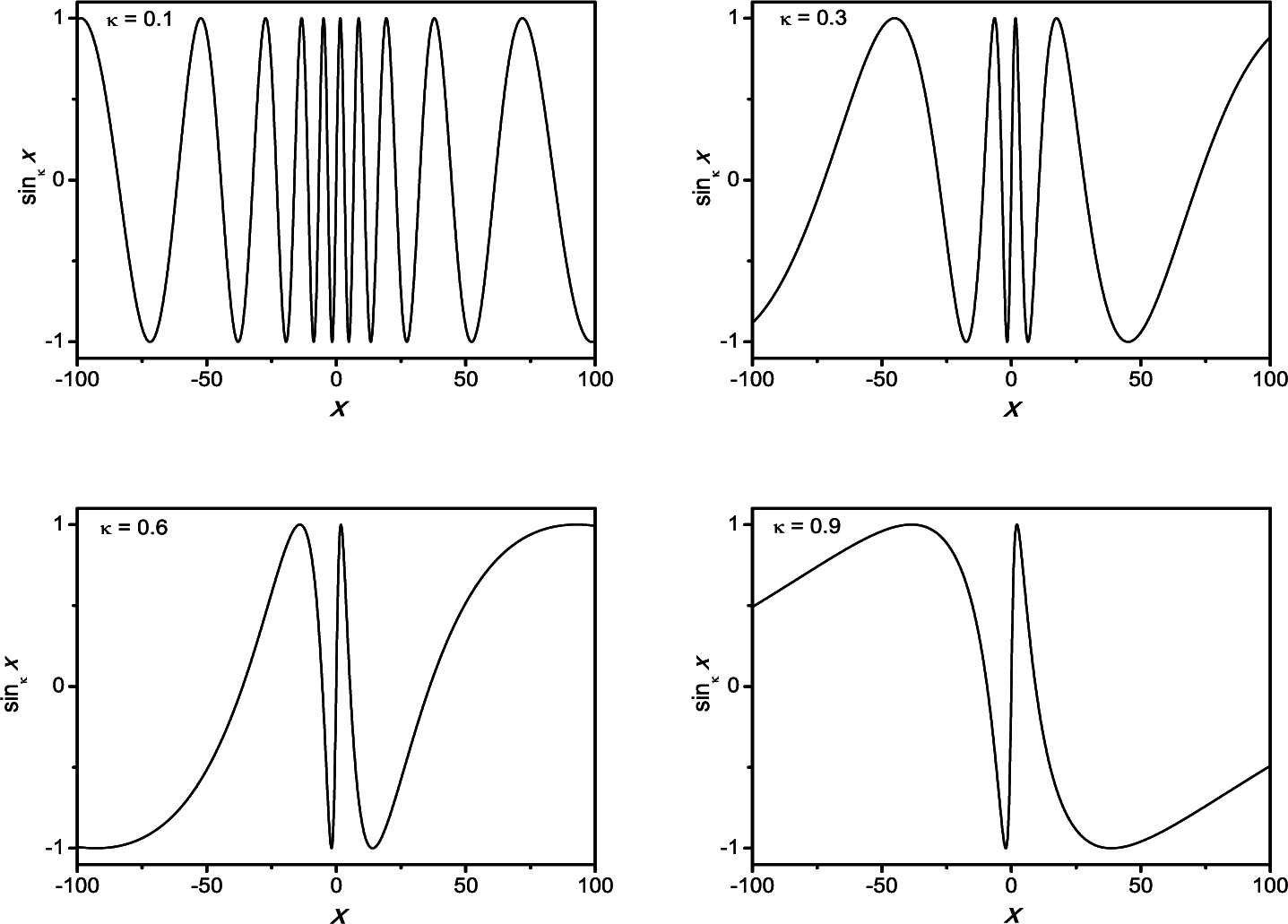
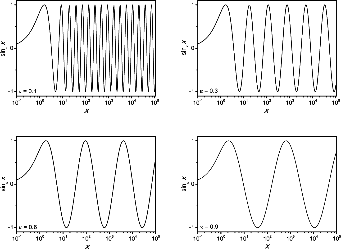
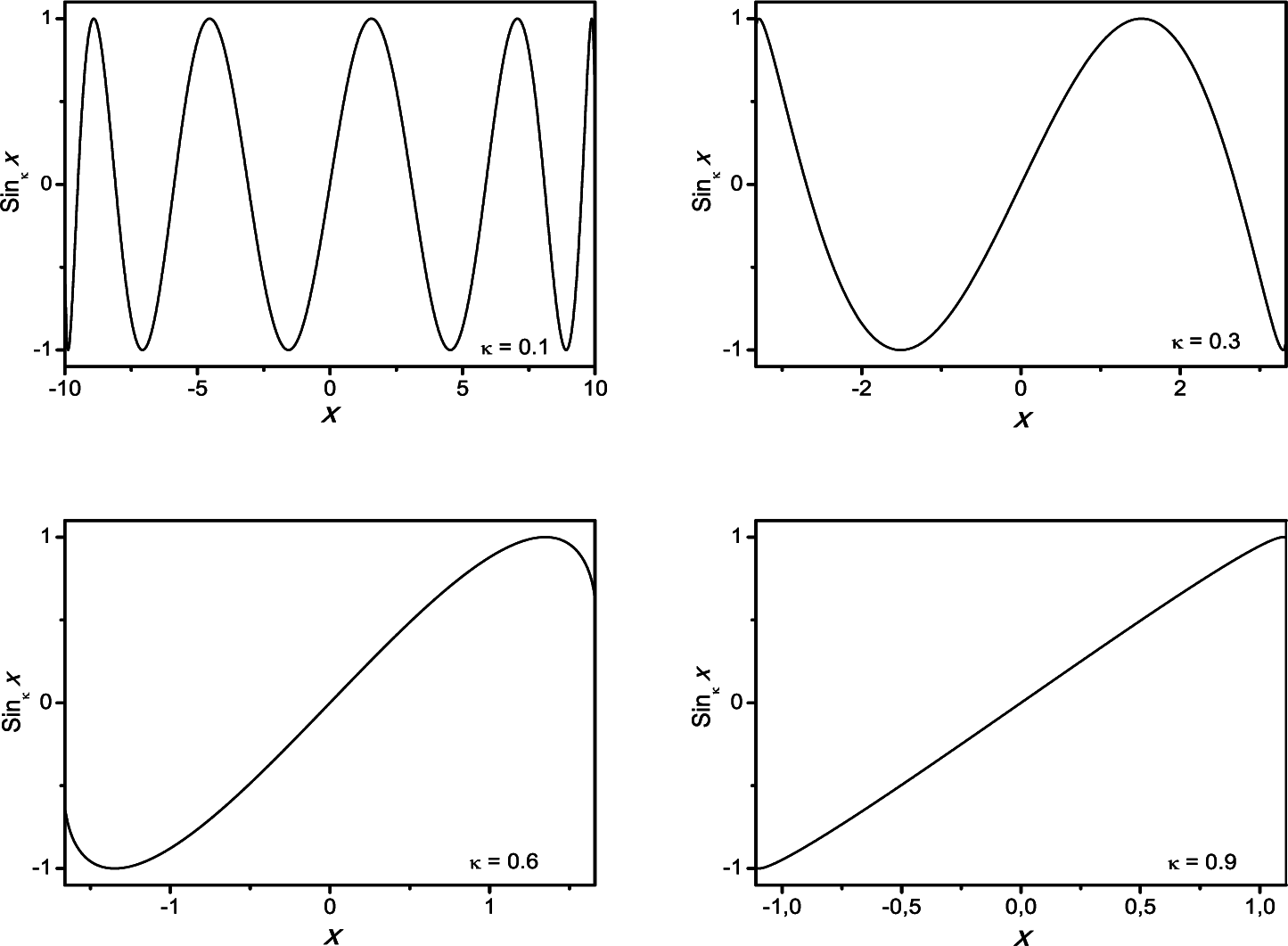
3. Euler Formula and κ-Cyclic Trigonometric Functions

In this section, we present two possible κ-deformations of the Euler formula for the complex exponential and derive the corresponding trigonometric functions in the framework of the κ-formalism.

3.1. First Case

The first possible definition of the complex κ-exponential is given by:

$${\left({\exp }_{\kappa }x\right)}^i={\exp }_{\kappa }\left(i^{\left\{\kappa \right\}}\otimes x\right)\equiv \exp \left(i{x}_{\left\{\kappa \right\}}\right),$$

(54)

where:

$$i^{\left\{\kappa \right\}}=i\frac{\sin \kappa }{\kappa }.$$

(55)

The complex number z = (exp_k x)ⁱ describes the unitary circle in the complex plane like the function exp(ix) does. Therefore, Function (54) has a unitary modulus for any x ∊ ℜ. However, noting that |x| > |x_{κ}|, as well as the difference |x − x_{κ}| increases as |x| → ∞, it follows that the circle is revolving around slowly as |x| grows. This implies that the function (exp_κ x)ⁱ maps the unitary circle with a period that increases as |x| increases.

We introduce the first family of κ-deformed cyclic functions ${\mathcal{C}}^{\left(1\right)}\equiv \left\{{\sin }_{\kappa }x,{\cos }_{\kappa }x,{\tan }_{\kappa }x\right\}$ according to the Euler formula:

$${\left({\exp }_{\kappa }x\right)}^i={\cos }_{\kappa }x+i{\sin }_{\kappa }x.$$

(56)

By observing that:

$${\left[{\left({\exp }_{\kappa }x\right)}^i\right]}^{*}={\left({\exp }_{\kappa }\left(-x\right)\right)}^i,$$

(57)

where * means the complex conjugate; we obtain:

$$\begin{array}{l}{\sin }_{\kappa }x-\frac{{\left({\exp }_{\kappa }x\right)}^i-{\left({\exp }_{\kappa }\left(-x\right)\right)}^i}{2i},\\ {\cos }_{\kappa }x=\frac{{\left({\exp }_{\kappa }x\right)}^i+{\left({\exp }_{\kappa }\left(-x\right)\right)}^i}{2},\\ {\tan }_{\kappa }x=\frac{{\sin }_{\kappa }x}{{\cos }_{\kappa }x},\end{array}$$

(58)

and accounting for Equation (54), the functions in ${\mathrm{C}}^{\left(1\right)}$ are related to the standard trigonometric functions as:

$$\begin{array}{cc}{\sin }_{\kappa }x=\sin x_{\left\{\kappa \right\}},& {\cos }_{\kappa }x=\text{cos}{x}_{\kappa },\end{array}$$

(59)

that is, the κ-trigonometric functions of a real number x coincide with the corresponding standard trigonometric functions of the κ-number x_{κ}. As a consequence, the κ-cyclic functions are periodic like the standard functions sin x and cos x, although their period is not constant, but increases for |x| → ∞, in agreement with our previous considerations.

This can be easily verified observing that:

$$\begin{array}{cc}{\sin }_{\kappa }x={\sin }_{\kappa }{x}^{\prime }& \text{when}{x}^{\prime }={\left(x_{\left\{\kappa \right\}}+2n\pi \right)}^{\left\{\kappa \right\}},\end{array}$$

(60)

so that, for large x, we obtain:

$$\Delta \ln x\simeq 2n\pi \kappa ,$$

(61)

where ∆ ln x = ln x′ − ln x. This behavior is shown in Figure 1, where we plot the function sin_κ x for several values of κ. The same picture is reproduced in Figure 2 in a linear-log scale, where it is clear as the periods become constant for large |x|, whilst it grows as the parameter κ increases, in agreement with Equation (61).

Within the κ-formalism, it is straightforward to verify that the functions in ${\mathrm{C}}^{\left(1\right)}$ preserve the algebraic structure of the ordinary cyclic functions. The standard relations are recovered in the κ → 0 limit. For example:

$$\begin{array}{l}{\sin }_{\kappa }^{2}x+{\cos }_{\kappa }^{2}x=1,\\ {\sin }_{\kappa }\left(x\oplus y\right)={\sin }_{\kappa }{\cos }_{\kappa }y+{\cos }_{\kappa }x{\sin }_{\kappa }y,\\ {\sin }_{\kappa }\left(2^{\left\{\kappa \right\}}\otimes x\right)=2{\sin }_{\kappa }x{\cos }_{\kappa }y,\\ {\left({\cos }_{\kappa }x+i\sin \kappa x\right)}^n={\cos }_{\kappa }\left(n^{\left\{\kappa \right\}}\otimes x\right)+i{\sin }_{\kappa }\left(n^{\left\{\kappa \right\}}\otimes x\right).,\end{array}$$

(62)

as well as the main κ-derivative relations:

$$\begin{array}{l}\frac{d}{d_{\kappa }x}{\sin }_{\kappa }x={\cos }_{\kappa }x,\\ \frac{d}{d_{\kappa }x}{\cos }_{\kappa }x=-{\sin }_{\kappa }x,\\ \frac{d}{d_{\kappa }x}{\tan }_{\kappa }x=-\frac{1}{{\cos }_{\kappa }^{2}x},\end{array}$$

(63)

to show a few.

Finally, let us observe that the functions sin_κ x and cos_κ x can be derived starting from the following κ-differential equation:

$$\frac{d^{2}u\left(x\right)}{d_{\kappa }{x}^2}+a_{\left\{\kappa \right\}}^{2}u\left(x\right)=0,$$

(64)

with a_{κ} a constant, which can be rewritten in the form of a Sturm-Liouville equation:

$$\frac{d}{dx}\left(\sqrt{1+{\kappa }^2{x}^2}\frac{du\left(x\right)}{dx}\right)+\frac{a_{\left\{\kappa \right\}}^2}{\sqrt{1+{\kappa }^2{x}^2}}u\left(x\right)=0,$$

(65)

corresponding to Equation (4) with $p\left(x\right)=\sqrt{1+{\kappa }^2{x}^2},q\left(x\right)=0$ and the weight function $w\left(x\right)=1/\sqrt{1+{\kappa }^2{x}^2}$. It is easy to verify that a solution of Equation (65), fulfilling the boundary conditions:

$$u\left(-u\right)=u\left(h\right)=0,$$

(66)

is given by

$$u\left(x\right)\equiv {\phi }_n\left(x\right)=A{\sin }_{\kappa }\left(a_n\otimes x\right),$$

(67)

while a solution that fulfills the condition:

$$u^{\prime }\left(-h\right)=u^{\prime }\left(h\right)=0,$$

(68)

where u′ (x) = du(x)/dx is:

$$u\left(x\right)\equiv {\varphi }_n\left(x\right)=A{\text{cos}}_{\kappa }\left(a_n\otimes x\right),$$

(69)

provided that a_n ≡ (nπ/h_{κ})^{κ}.

3.2. Second Case

The second generalization of the complex κ-exponential follows by replacing the argument of the κ-exponential with a purely imaginary quantity: x → ix. This definition was firstly introduced in [32], and the resulting complex κ-exponential reads:

$${\exp }_{\kappa }\left(i\kappa \right)\equiv \exp {\left(ix\right)}_{\left\{\kappa \right\}}=\exp \left(i{x}_{\left[\kappa \right]}\right),$$

(70)

where the numbers x_[κ] and their dual x^[κ] are given by:

$$\begin{array}{cc}{x}_{\left[\kappa \right]}=\frac{1}{\kappa }\arcsin \left(\kappa x\right),& x^{\left[\kappa \right]}=\frac{1}{\kappa }\sin \left(\kappa x\right),\end{array}$$

(71)

with (x^[κ])_[κ] = (x_[κ])^[κ] = x. They are related to the numbers x_{κ}, that is x_[κ] = x_{κ′}, according to the parameter transformation:

$$\kappa \to {\kappa }^{\prime }=i\kappa ,$$

(72)

as well as, by using the scaling properties of exp_κ x, Equation (70) is related to Equation (54) as:

$${\exp }_{\kappa }\left(ix\right)={\left({\exp }_{i\kappa }x\right)}^i\equiv {\left({\exp }_{{\kappa }^{\prime }}x\right)}^i.$$

(73)

However, Function (70) is characterized by an unitary modulus for |x| ≤1/|κ| while, for |x| > 1/|κ|, the value of |exp_κ(i x)| increases monotonically:

$$\begin{array}{cc}|{\exp }_{\kappa }\left(ix\right)|=1& \text{for}|x|\le 1/|\kappa |,\end{array}$$

(74)

$$\begin{array}{cc}|{\exp }_{\kappa }\left(ix\right)|={\left(\kappa x+\sqrt{{\kappa }^2{x}^2-1}\right)}^{1/\kappa }& \text{for}|x|>1/|\kappa |.\end{array}$$

(75)

According to the Euler formula, we introduce a second family of κ-deformed trigonometric functions ${\mathcal{C}}^{\left(2\right)}\equiv \left\{{\sin }_{\kappa }x,{\mathrm{Cos}}_{\kappa }x,{\text{Tan}}_{\kappa }x\right\}$ given by:

$${\exp }_{\kappa }\left(ix\right)={\mathrm{Cos}}_{\kappa }x+i{\mathrm{Sin}}_{\kappa }x,$$

(76)

and in this case, the definitions of the κ-cyclic functions become:

$$\begin{array}{l}{\mathrm{Sin}}_{\kappa }x=\frac{{\exp }_{\kappa }\left(i\kappa \right)-{\exp }_{\kappa }\left(-ix\right)}{2i},\\ {\mathrm{Sin}}_{\kappa }x=\frac{{\exp }_{\kappa }\left(ix\right)+{\exp }_{\kappa }\left(-ix\right)}{2},\\ {\mathrm{Tan}}_{\kappa }x=\frac{{\mathrm{Sin}}_{\kappa }x}{{\mathrm{Cos}}_{\kappa }x}.\end{array}$$

(77)

Remark that, as follows from Equation (70), the functions in ${\mathrm{C}}^{\left(2\right)}$ are linked to the standard trigonometric functions as:

$$\begin{array}{cc}{\mathrm{Sin}}_{\kappa }x=\sin x_{\left[\kappa \right]},& {\mathrm{Cos}}_{\kappa }x=\cos x_{\left[\kappa \right]}.\end{array}$$

(78)

Notice that the quantities [x]_κ take real values for |x| ≤ 1/|κ|, and consequently, like exp_κ(ix), the functions in ${\mathrm{C}}^{\left(2\right)}$ have a real image and modulus unitary only in the interval |x| ≤ 1/|κ|. In additions, the wavelength of Sin_κx and Cos_κx reduces for |x| → 1/|κ| as well as it increases as |κ| grows. For |κ| > 1/4, the periods of these functions become grater than their real domain, and the functions cease to be periodic.

These facts are shown in Figure 3, where we plot the shape of Sin_κx iven in Equation (77), in its real domain, for several values of the deformation parameter κ.

In passing, let us observe that the relation (ix)_{κ} = ix_[κ] introduces a different definition for the κ-sum and the κ-product, which follows from Equation (33) with f (x) = κ⁻¹ arcsin(κx). They are given by:

$$x\overline{\oplus }y=\frac{1}{\kappa }\sin \left(\arcsin \left(\kappa x\right)+\arcsin \left(\kappa y\right)\right),$$

(79)

$$x\overline{\oplus }y=\frac{1}{\kappa }\sin \left(\frac{1}{\kappa }\arcsin \left(\kappa x\right)\cdot \arcsin \left(\kappa y\right)\right),$$

(80)

as well as the κ-derivative becomes:

$${\left(\frac{d}{dx}\right)}_{\left[\kappa \right]}\equiv \frac{d}{d_{\left[\kappa \right]}x}=\frac{dx}{d{x}_{\left[\kappa \right]}}\frac{d}{dx}=\sqrt{1-{\kappa }^2{x}^2}\frac{d}{dx},$$

(81)

so that d_[κ]x = dx_[κ].

Consequently, all of the fundamental relations of the trigonometric functions, including the related calculus, turn out to be re-obtained in the corresponding κ-formalism. For instance, we have:

$$\begin{array}{l}{\mathrm{Sin}}_{\kappa }^{2}x+{\mathrm{Cos}}_{\kappa }^{2}x=1,\\ {\mathrm{Sin}}_{\kappa }\left(x\overline{\oplus }y\right)={\mathrm{Sin}}_{\kappa }x{\mathrm{Cos}}_{\kappa }y+{\mathrm{Cos}}_{\kappa }y,\\ {\mathrm{Sin}}_{\kappa }\left(2^{\left[\kappa \right]}\overline{\otimes }x\right)=2{\mathrm{Sin}}_{\kappa }x{\mathrm{Cos}}_{\kappa }y,\\ {\left({\mathrm{Cos}}_{\kappa }x+i{\mathrm{Sin}}_{\kappa }x\right)}^n={\mathrm{Cos}}_{\kappa }\left(n^{\left[\kappa \right]}\overline{\otimes }x\right)+i{\mathrm{Sin}}_{\kappa }\left(n^{\left[\kappa \right]}\overline{\otimes }x\right),\end{array}$$

(82)

as well as:

$$\begin{array}{l}\frac{d}{d_{\left[\kappa \right]}x}{\mathrm{Sin}}_{\kappa }x={\mathrm{Cos}}_{\kappa }x,\\ \frac{d}{d_{\left[\kappa \right]}x}{\mathrm{Cos}}_{\kappa }x=-{\mathrm{Sin}}_{\kappa }x,\\ \frac{d}{d_{\left[\kappa \right]}x}{\mathrm{Tan}}_{\kappa }\left(x\right)=-\frac{1}{{\mathrm{Cos}}_{\kappa }^{2}x},\end{array}$$

(83)

and so on.

Finally, we can obtain the functions Sin_κx and Cos_κx from a Sturm-Liouville problem. In fact, they are related to the following differential equation:

$$\frac{d^{2}u\left(x\right)}{d_{\left[\kappa \right]}{x}^2}+a_{\left[\kappa \right]}^{2}u\left(x\right)=0,$$

(84)

which coincides with Equation (4) with $p\left(x\right)=\sqrt{1-{\kappa }^2{x}^2},q\left(x\right)=0$ and $w\left(x\right)=1/\sqrt{1-{\kappa }^2{x}^2}$. A solution of Equation (84) fulfilling the boundary condition u(−h) = u(h) = 0 is given by:

$$u\left(x\right)\equiv {\overline{\phi }}_n=A{\mathrm{Sin}}_{\kappa }\left(a_n\overline{\otimes }x\right),$$

(85)

while under the condition u′(−h) = u′(h) = 0, the solution is:

$$u\left(x\right)\equiv {\overline{\varphi }}_n=A{\mathrm{Cos}}_{\kappa }\left(a_n\overline{\otimes }x\right),$$

(86)

where a_n = (nπ/h_[κ])^[κ].

4. Orthogonality and Completeness Relations

In this section, we discuss the orthogonality and completeness relations for the two family ${\mathrm{C}}^{\left(1\right)}$ and ${\mathrm{C}}^{\left(2\right)}$ of the κ-trigonometric functions.

Firstly, we introduce in the space of the square-integrable functions L²[−h, h] the scalar product:

$${\langle f,g\rangle }_w={\displaystyle \underset{-h}{\overset{h}{\int }}f\left(x\right)}g\left(x\right)w\left(x\right)dx,$$

(87)

where w(x) is a suitable weight function. When $w\left(x\right)=1/\sqrt{1+{\kappa }^2{x}^2}$, Equation (87) reduces to the κ-integral (50). Therefore, we define the scalar product in the κ-formalism according to:

$${\langle f,g\rangle }_{\left\{\kappa \right\}}={\displaystyle \underset{-h}{\overset{h}{\int }}f\left(x\right)}g\left(x\right)d_{\left\{\kappa \right\}}x.$$

(88)

Let Φ⁽¹⁾ be the set of square-integrable functions L²[−h, h] given by:

$${\Phi }^{\left(1\right)}=\left\{{\phi }_n\equiv \frac{1}{\sqrt{h}}{\text{sin}}_{\kappa }\left(a_n\otimes x\right),{\varphi }_m\equiv \frac{1}{\sqrt{h}}{\cos }_{\kappa }\left(a_m\otimes x\right)\right\},$$

(89)

where a_n are given constant, with n = 1, 2, … and m = 0, 1,

Accounting for the results presented in Section 3.1, it is straightforward to show that forms a set of orthogonal functions in L²[−h, h] when:

$$a_n=\frac{1}{\kappa }\sinh \left(\frac{n\pi {\kappa }^2}{\text{arcsinh}\left(\kappa h\right)}\right)\equiv {\left(\frac{n\pi }{h_{\left\{\kappa \right\}}}\right)}^{\left\{\kappa \right\}}.$$

(90)

This can be easily verified by considering, for instance, the following scalar product:

$$\begin{array}{l}\langle {\phi }_n,{\varphi }_m\rangle ={\displaystyle \underset{-h}{\overset{h}{\int }}{\sin }_{\kappa }}\left(a_n\otimes x\right){\cos }_{\kappa }\left(a_m\otimes x\right)d_{\left\{\kappa \right\}}x\\ ={\displaystyle \underset{-h}{\overset{h}{\int }}{\sin }_{\kappa }}{\left(a_n\otimes x\right)}_{\kappa }\cos \left(a_m\otimes x\right)d{x}_{\left\{\kappa \right\}}\\ ={\displaystyle \underset{-h}{\overset{h}{\int }}\sin }\left({\left(a_n\right)}_{\left\{\kappa \right\}}{x}_{\left\{\kappa \right\}}\right){\cos }_{\kappa }\left({\left(a_m\right)}_{\left\{\kappa \right\}}{x}_{\left\{\kappa \right\}}\right)d{x}_{\left\{\kappa \right\}},\end{array}$$

(91)

and denoting y = x_{κ} and $a_n^{\prime }={\left(a_n\right)}_{\left\{\kappa \right\}}$, we obtain:

$${\langle {\phi }_n,{\varphi }_m\rangle }_{\left\{\kappa \right\}}=\underset{-h_{\left\{\kappa \right\}}}{\overset{h_{\left\{\kappa \right\}}}{\int }}\sin \left(a_n^{\prime }y\right)\cos \left(a_m^{\prime }y\right)dy,$$

(92)

which coincides with the orthogonality condition between the sine and the cosine functions in the standard Fourier series theory. Orthogonality is recovered for $a_n^{\prime }=n\pi /h_{\left\{\kappa \right\}}$, which implies Equation (90).

Actually, this was expected, since, as is known, any pair of solutions of a Sturm-Liouville problem belonging to different eigenvalues is orthogonal with respect to an opportunely weighed scalar product.

In the same way, the completeness relation follows from the Sturm-Liouville theory and it is stated by the relation:

$${\displaystyle \sum _{n=1}^{\infty }{u}_n\left(x\right)u_n\left(y\right)w\left(x\right)=\delta \left(x-y\right)},$$

(93)

where u_n(x) are eigenfunctions of the given problem. In order to prove the completeness relation for the system ${\mathrm{C}}^{\left(1\right)}$ we start by the well-known relation:

$$\frac{2}{h}\underset{n=1}{\overset{\infty }{\Sigma }}\sin \left(\frac{n\pi }{h}x\right)\sin \left(\frac{n\pi }{h}y\right)=\delta \left(x-y\right).$$

(94)

Substituting x → x_{κ}, the sine function transforms as:

$$\begin{array}{l}\sin \left(\frac{n\pi }{h}x\right)\to \sin \left(\frac{n\pi }{h}{x}_{\left\{\kappa \right\}}\right)\\ ={\sin }_{\kappa }{\left(\frac{n\pi }{h}{x}_{\left\{\kappa \right\}}\right)}^{\left\{\kappa \right\}}\\ \equiv {\sin }_{\kappa }\left(a_n\otimes x\right),\end{array}$$

(95)

with a_n given in Equation (90).

On the other hand, the right-hand side of Equation (94) changes in:

$$\delta \left(x-y\right)\to \delta \left(x_{\left\{\kappa \right\}}-y_{\left\{\kappa \right\}}\right)=\delta \left(x-y\right)\sqrt{1+{\kappa }^2{x}^2},$$

(96)

according to the following propriety of the Dirac delta function:

$$\delta \left(f\left(x\right)\right)=\underset{i}{\Sigma }\frac{\delta \left(x-x_i\right)}{df\left(x\right)/dx{|}_{x=x_i}}.$$

(97)

By inserting Equations (95) and (96) into Equation (94), we finally obtain:

$$\frac{2}{h}\underset{n=1}{\overset{\infty }{\Sigma }}{\sin }_{\kappa }\left(a_n\otimes x\right){\sin }_{\kappa }\left(a_n\otimes y\right)\frac{1}{\sqrt{1+{\kappa }^2{x}^2}}=\delta \left(x-y\right),$$

(98)

which is the required completeness relation for the κ-sine functions. Similar arguments can be applied to derive the completeness relation of the κ-cosine functions stated in:

$$\frac{2}{h}\underset{n=0}{\overset{\infty }{\Sigma }}{\cos }_{\kappa }\left(a_n\otimes x\right){\cos }_{\kappa }\left(a_n\otimes y\right)\frac{1}{\sqrt{1+{\kappa }^2{x}^2}}=\delta \left(x-y\right).$$

(99)

Passing to the family ${\mathrm{C}}^{\left(2\right)}$, we do not have a significant difference with respect to the arguments discussed above. Therefore, we can affirm that the set of functions:

$${\Phi }^{\left(2\right)}=\left\{{\overline{\phi }}_n\equiv \sqrt{\frac{2}{h}}{\mathrm{Sin}}_{\kappa }\left(a_n\overline{\otimes }x\right),{\overline{\varphi }}_m\equiv \sqrt{\frac{2}{h}}{\mathrm{Cos}}_{\kappa }\left(a_m\overline{\otimes }x\right)\right\},$$

(100)

with:

$$a_n=\frac{1}{\kappa }\sinh \left(\frac{n\pi {\kappa }^2}{\arcsin \left(\kappa h\right)}\right)\equiv {\left(\frac{n\pi }{h_{\left[\kappa \right]}}\right)}^{\left[\kappa \right]},$$

(101)

form a system orthonormal and completed in the space of the square-integrable functions L²(−h, h) ⊆ l²(−1/|κ|, 1/|k|).

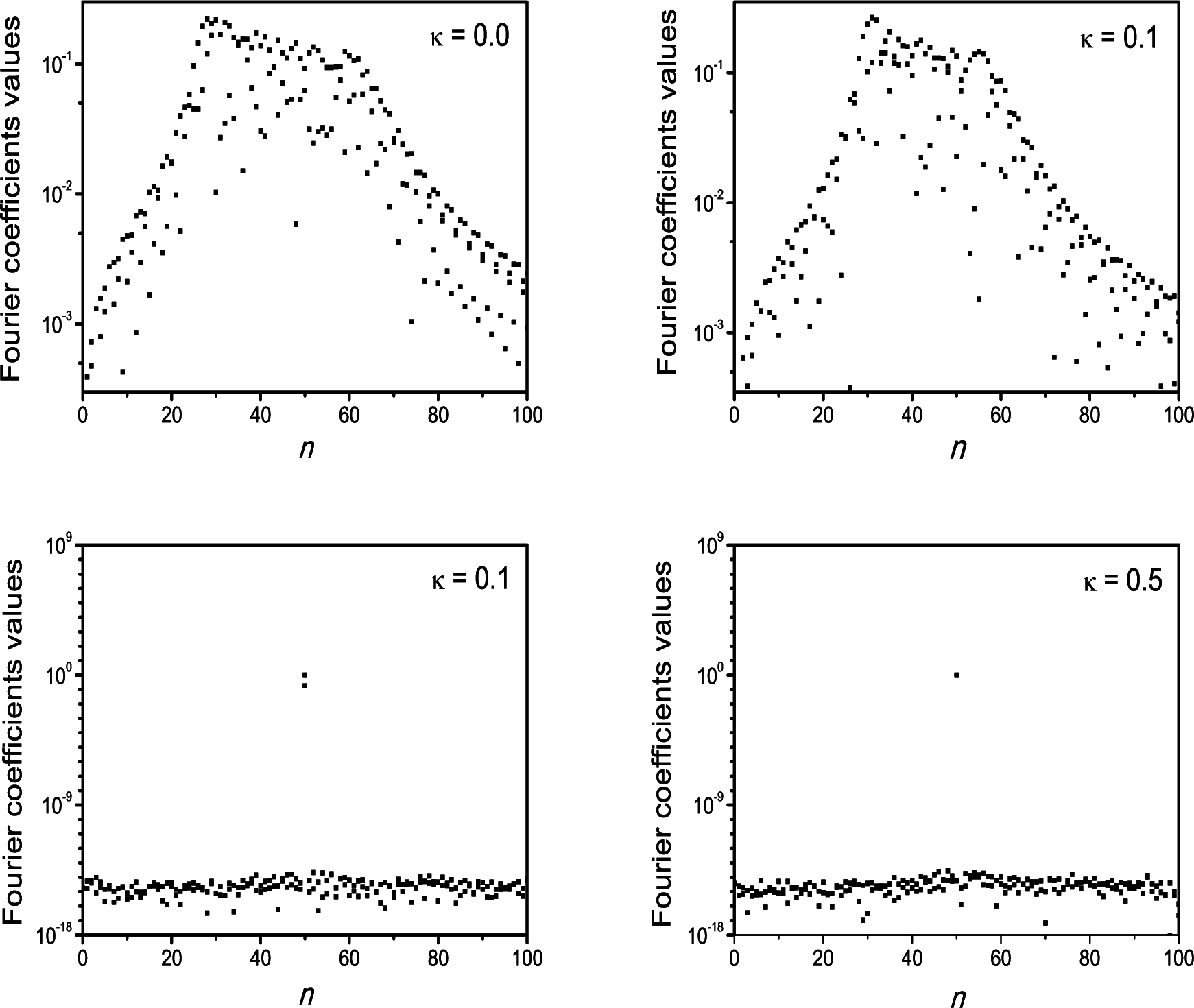
5. Generalized Fourier Series

In mathematical analysis, generalized Fourier series are introduced as special cases of decompositions over a given orthonormal basis of an inner product space.

By specializing to the present situation, any square-integrable function f (x) : (−h, h) → ℜ, satisfying the boundary conditions (66) with an odd parity, may be expanded in the κ-sine Fourier series with respect to the orthogonal base φ_n ∊ Φ⁽¹⁾ according to:

$$f\left(x\right)=\underset{n=1}{\overset{\infty }{\Sigma }}{s}_n{\sin }_{\kappa }\left(a_n\otimes x\right),$$

(102)

where the coefficients s_n are unique constants given by:

$$\begin{array}{cc}{s}_n={\langle f\left(x\right),{\phi }_n\left(x\right)\rangle }_{\left\{\kappa \right\}}\equiv \sqrt{\frac{2}{h}}\underset{0}{\overset{h}{\int }}f\left(x\right){\sin }_{\kappa }\left(a_n\otimes x\right)d_{\left\{\kappa \right\}}x,& n=1,2,\dots .\end{array}$$

(103)

In the same way, any square-integrable function f(x) : (−h, h) → ℜ, satisfying the boundary conditions (68) with an even parity, may be expanded in the κ-cosine Fourier series with respect to the orthogonal base ϕ_n ∊ Φ⁽¹⁾, according to:

$$f\left(x\right)=c_0+\underset{n=1}{\overset{\infty }{\Sigma }}{c}_n{\text{cos}}_{\kappa }\left(a_n\otimes x\right),$$

(104)

where the coefficients c₀ and c_n are unique constants given by:

$$c_0={\langle f\left(x\right),1\rangle }_{\left\{\kappa \right\}}\equiv \sqrt{\frac{2}{h}}\underset{0}{\overset{h}{\int }}f\left(x\right)d_{\left\{\kappa \right\}}x,$$

(105)

$$\begin{array}{cc}{c}_n={\langle f\left(x\right),{\phi }_n\left(x\right)\rangle }_{\left\{\kappa \right\}}\equiv \sqrt{\frac{2}{h}}\underset{0}{\overset{h}{\int }}f\left(x\right){\cos }_{\kappa }\left(a_n\otimes x\right)d_{\left\{\kappa \right\}}x,& n=1,2,\dots ,\end{array}$$

(106)

and more in general, any square-integrable function f(x): (−h, h) → ℜ, with no well-defined parity, may be expanded in the κ-Fourier series with respect to the orthogonal base Φ(¹⁾, according to:

$$f\left(x\right)=c_0+\underset{n=1}{\overset{\infty }{\Sigma }}\left(s_n{\sin }_{\kappa }\left(a_n\otimes x\right)+c_n{\cos }_{\kappa }\left(a_n\otimes x\right)\right),$$

(107)

with coefficients given in Equations (103),(105) and (106).

The κ-Fourier series (107) can be eventually written in the complex form by using formulas (58) as:

$$f\left(x\right)=\underset{n=-\infty }{\overset{\infty }{\Sigma }}{\gamma }_n{\left({\exp }_{\kappa }\left(a_n\otimes x\right)\right)}^i,$$

(108)

where the complex Fourier coefficients are given by:

$${\gamma }_n=\frac{1}{\sqrt{2h}}\underset{0}{\overset{h}{\int }}f\left(x\right){\left({\exp }_{\kappa }\left(a_n\otimes x\right)\right)}^i{d}_{\left\{\kappa \right\}}x,$$

(109)

and are related to the real Fourier coefficients in γ_−n = (c_n − i s_n)/2 and Y_n = (c_n + i s_n)/2.

The completeness of the system implies the Parseval relation for the coefficients c_n and s_n:

$$c_0^2+\underset{n=1}{\overset{\infty }{\Sigma }}\left(c_n^2+s_n^2\right)=\frac{2}{h}\underset{0}{\overset{h}{\int }}f{\left(x\right)}^2{d}_{\left\{\kappa \right\}}x,$$

(110)

or more in general, for any two real functions f(x) and g(x) belonging to L²(−h, h) and than expandable in the complex Fourier series with coefficients γ_n and δ_n, we have:

$$\underset{n=-\infty }{\overset{\infty }{\Sigma }}{\gamma }_n{\delta }_n^{*}=\frac{1}{2h}\underset{0}{\overset{h}{\int }}f\left(x\right)g\left(x\right)d_{\left\{\kappa \right\}}x,$$

(111)

from which the Parseval theorem (110) follows for f(x) = g(x).

At this point, it is worth stating that the κ-Fourier series (107) actually is equivalent to a standard Fourier series of a suitably-transformed function. In fact, by means of the substitution x → x^{κ}, it is straightforward to change Equation (107) in:

$$f\left(x^{\left\{\kappa \right\}}\right)=c_0+\underset{n=1}{\overset{\infty }{\Sigma }}\left(s_n\sin \left(a_n^{\prime }x\right)+c_n\cos \left(a_n^{\prime }x\right)\right),$$

(112)

where the Fourier coefficients are now given by:

$$\begin{array}{cc}{s}_n=\sqrt{\frac{2}{h}}\underset{0}{\overset{h^{\left\{\kappa \right\}}}{\int }}f\left(x^{\kappa }\right)\sin \left(a_n^{\prime }x\right)dx,& n=1,2,,\dots ,\end{array}$$

(113)

$$\begin{array}{cc}{c}_n=\sqrt{\frac{2}{h}}\underset{0}{\overset{h^{\left\{\kappa \right\}}}{\int }}f\left(x^{\kappa }\right)\cos \left(a_n^{\prime }x\right)dx,& n=0,1,\dots ,\end{array}$$

(114)

with $a_n^{\prime }=2\pi n/h$. They coincide with the well-known relations of the standard Fourier theory for the expansion of the function f(x^{κ}).

Finally, all of the above considerations still hold, opportunely modified, for the set of functions ${\mathcal{C}}^{\left(2\right)}$. Explicitly, any square-integrable function f(x): (−h, h) ⊆ (−1/|κ|, 1/|κ|) → ℜ admits a decomposition in the orthogonal base Φ⁽²⁾ as:

$$f\left(x\right)={\overline{c}}_0+\underset{n=1}{\overset{\infty }{\Sigma }}\left({\overline{s}}_n{\mathrm{Sin}}_{\kappa }\left(a_n\overline{\otimes }x\right)+{\overline{c}}_n{\mathrm{Cos}}_{\kappa }\left(a_n\overline{\otimes }x\right)\right),$$

(115)

where the coefficients ${\overline{s}}_n$ and ${\overline{c}}_n$ are the unique constants given by:

$$\begin{array}{cc}{\overline{s}}_n={\langle f\left(x\right),{\overline{\phi }}_n\left(x\right)\rangle }_{\left[\kappa \right]}\equiv \sqrt{\frac{2}{h}}\underset{0}{\overset{h}{\int }}f\left(x\right){\mathrm{Sin}}_{\kappa }(a_n\overline{\otimes }x)d_{\left[\kappa \right]}x,& n=1,2,\dots ,\end{array}$$

(116)

$$\begin{array}{cc}{\overline{c}}_n={\langle f\left(x\right),{\overline{\phi }}_n\left(x\right)\rangle }_{\left[\kappa \right]}\equiv \sqrt{\frac{2}{h}}\underset{0}{\overset{h}{\int }}f\left(x\right){\mathrm{Cos}}_{\kappa }(a_n\overline{\otimes }x)d_{\left[\kappa \right]}x,& n=0,1,2,\dots ,\end{array}$$

(117)

with ${\overline{\varphi }}_0\left(x\right)\equiv 1$ and fulfilling the Parseval relation:

$${\overline{c}}_0^2+\underset{n=1}{\overset{\infty }{\Sigma }}\left({\overline{c}}_n^2+{\overline{s}}_n^2\right)=\frac{2}{h}\underset{0}{\overset{h}{\int }}f{\left(x\right)}^2{d}_{\left[\kappa \right]}x.$$

(118)

Furthermore, in this case, the κ-Fourier series (115) of the function f (x) is equivalent to a standard Fourier series of the transformed function f (x^[κ]).

6. Final Remarks

In this paper, we have studied two possible generalizations of the complex exponential in the framework of the κ-formalism. They are given by:

$$\exp \left(ix\right)\to {\left({\exp }_{\kappa }x\right)}^i\equiv \exp {\left(f_{\kappa }^{\left(m\right)}\left(x\right)\right)}^i,$$

(119)

where the generating function $f_{\kappa }^{\left(m\right)}\left(x\right)$ is defined by:

$$f_{\kappa }^{\left(1\right)}\left(x\right)=\frac{1}{\kappa }\text{arcsinh}\left(\kappa x\right),$$

(120)

in the first formalism and by:

$$f_{\kappa }^{\left(2\right)}\left(x\right)=\frac{1}{\kappa }\text{arcsinh}\left(\kappa x\right),$$

(121)

in the second formalism.

The same functions introduce two different Abelian structures on the real κ-numbers x_{κ} and x_[κ], which are endowed by a generalized sum and product, defined as (in the text, for the sake of notations, the generalized operations associated with the κ-numbers x_[κ] have been denoted by $\overline{\oplus }$ and $\overline{\otimes }$, respectively):

$$x\oplus y=f_{\kappa }^{-1}\left(f_{\kappa }\left(x\right)+f_{\kappa }\left(y\right)\right),$$

(122)

$$x\otimes y=f_{\kappa }^{-1}\left(f_{\kappa }\left(x\right)\cdot f_{\kappa }\left(y\right)\right),$$

(123)

where $f_{{}_{\kappa }}\equiv f_{\kappa }^{\left(1\right)}$ or $f_{{}_{\kappa }}\equiv f_{\kappa }^{\left(2\right)}$, respectively.

According to the Euler formula, we have introduced two families of κ-deformed cyclic functions with different properties. The family ${\mathrm{C}}^{(2)}$ is formed by oscillating functions defined on the whole ℜ with a period that increases as |x| → ∞. They turn out to be asymptotically log-periodic. Differently, the family ${\mathrm{C}}^{\left(2\right)}$ is formed by oscillating functions defined in the limited region (−1/|κ|, 1/|κ|)with a period that shrinks as |x| → 1/|κ|. In both cases, we have verified that the main algebraic relations of the standard trigonometric functions are preserved within the corresponding κ-formalism.

We have introduced two systems of κ-deformed cyclic functions Φ^(m) related to two different Sturm-Liouville problems. Orthogonality and completeness relations for the systems Φ^(m) are then obtained in the framework of the Sturm-Liouville theory and have been used to introduce two different κ-deformed Fourier series in the space of the square-integrable functions in L²(−h, h) and L²(−1/|κ|, 1/|κ|) respectively. In both cases, the corresponding κ-Fourier series can be recast in an ordinary Fourier series of a suitably κ-deformed function.

In spite of this, the present formalism can be fruitfully applied to the fractional analysis of functions defined in a fractal space, a subject that has been raising certain interest in the recent literature [35–38]. We conclude this paper by presenting briefly a possible application of the κ-Fourier expansion based on the system of functions for the study of log-periodic oscillating phenomena. This is a typical behavior that characterizes a wide class of self-similar systems having discrete scaling invariance [39]. It has been observed in different situations characterized by the presence of geometrical fractals [40] or self-similarity distributions [41] and is often related to the renormalization-group problem [42].

Like in the standard Fourier analysis, where a periodic function may be decomposed into a superposition of harmonic modes, giving us information about the spectral composition of the underlying phenomena, log-periodic functions can be analyzed with the same purpose by means of the κ-cyclic functions belonging to ${\mathrm{C}}^{\left(1\right)}$. Without entering into the details of the problem, which are outside the scope of the present work, we just illustrate the potentiality of the method by considering the spectral decomposition of a trivial log-oscillating function, namely:

$$f\left(x\right)=\cos \left(2\pi m\log \left(x\right)\right).$$

(124)

In Figure 4, we report the absolute value of the first n = 100 Fourier coefficients s_n and c_n of Function (124), with m = 50, evaluated in the period [e, e²] (a) for κ = 0.0, corresponding to the standard case and (b) for κ = 0.1. Clearly, in both cases, a large dispersion of the coefficient values around the m = 50 harmonic is observed, although in (b), this dispersion is sensibly narrower than in (a). Thus, in this situation, it seems that there is not a significative advantage in the use of the κ-Fourier analysis with respect to the standard one. This occurs since the onset of the log-periodic behavior of the κ-cyclic functions arises in the asymptotic region and then is not yet established in the windows [e, e²]. However, taking advantage of the periodicity of f (x), we can analyze its spectrum equivalently in the highest region, namely [e¹⁹, e²⁰], as shown in (c). Here, the log-periodic behavior of the κ-sine and κ-cosine functions is almost exact, and as expected, the spectrum corresponds to that of an exact monochromatic oscillation with only the s₅₀ and c₅₀ coefficients different from zero. Actually, one should expect the sole coefficient c₅₀ to be different from zero, since, after all, we are decomposing a monochromatic cos - log function. The presence of both of the coefficients, is caused by the initial region where the functions φ_n and ϕ_n do not have a log-periodic behavior. This causes a phase shift between the analyzed function and the harmonic waves used in the expansions. This phase shift may be tuned by acting on the deformation parameter, as shown in (d), where the only harmonic, corresponding to c₅₀ = 1, exists.

References

1. Kaniadakis, G. Non-linear kinetics underlying generalized statistics. Physica A 2001, 296, 405–425. [Google Scholar]
2. Kaniadakis, G. Statistical mechanics in the context of special relativity. Phys. Rev. E 2002, 66, 056125. [Google Scholar]
3. Kaniadakis, G. Statistical mechanics in the context of special relativity. II. Phys. Rev. E 2005, 72, 036108. [Google Scholar]
4. Silva, R. The H-theorem in κ-statistics: Influence on the molecular chaos hypothesis. Phys. Lett. A 2006, 352, 17–20. [Google Scholar]
5. Wada, T. Thermodynamic stability conditions for nonadditive composable entropies. Cont. Mech. Thermodyn 2004, 16, 263–267. [Google Scholar]
6. Kaniadakis, G.; Scarfone, A.M. Lesche stability of κ-entropy. Physica A 2004, 340, 102–109. [Google Scholar]
7. Kaniadakis, G. Maximum entropy principle and power-law tailed distributions. Eur. Phys. J. B 2009, 70, 3–13. [Google Scholar]
8. Kaniadakis, G. Relativistic entropy and related Boltzmann kinetics. Eur. Phys. J. A 2009, 40, 275–287. [Google Scholar]
9. Naudts, J. Continuity of a class of entropies and relative entropies. Rev. Math. Phys 2004, 16, 809–822. [Google Scholar]
10. Scarfone, A.M.; Wada, T. Canonical partition function for anomalous systems described by the κ-entropy. Prog. Theor. Phys. Suppl 2006, 162, 45–52. [Google Scholar]
11. Scarfone, A.M.; Wada, T. Thermodynamic equilibrium and its stability for microcanonical systems described by the Sharma-Taneja-Mittal entropy. Phys. Rev. E 2005, 72, 026123. [Google Scholar]
12. Santos, A.P.; Silva, R.; Alcaniz, J.S.; Anselmo, D.H.A.L. Non-Gaussian effects on quantum entropies. Physica A 2012, 391, 2182–2192. [Google Scholar]
13. Guo, L.; Du, J. The κ-parameter and κ-distribution in κ-deformed statistics for the systems in an external field. Phys. Lett. A 2007, 362, 368–370. [Google Scholar]
14. Wada, T.; Suyari, H. kappa-generalization of Gauss’ law of error. Phys. Lett. A 2006, 348, 89–93. [Google Scholar]
15. Wada, T.; Scarfone, A.M. Asymptotic solutions of a nonlinear diffusive equation in the framework of κ-generalized statistical mechanics. Eur. Phys. J. B 2009, 70, 65–71. [Google Scholar]
16. Wada, T. A nonlinear drift which leads to kappa-generalized distributions. Eur. Phys. J. B 2010, 73, 287–291. [Google Scholar]
17. Lapenta, G.; Markidis, S.; Kaniadakis, G. Computer experiments on the relaxation of collisionless plasmas. J. Stat. Mech. Theory Exp 2009, 2009. [Google Scholar] [CrossRef]
18. Lapenta, G.; Markidis, S.; Marocchino, A.; Kaniadakis, G. Relaxion of relativistic plasmas under the effect of wave-particle interactions. Astrophys. J 2007, 666, 949–954. [Google Scholar]
19. Rossani, A.; Scarfone, A.M. Generalized kinetic equations for a system of interacting atoms and photons: Theory and simulations. J. Phys. A Math. Theor 2004, 37, 4955–4975. [Google Scholar]
20. Carvalho, J.C.; Silva, R.; do Nascimento, J.D., Jr.; Soares, B.B.; de Medeiros, J.R. Observational measurement of open stellar clusters: A test of Kaniadakis and Tsallis statistics. Europhys. Lett 2010, 91. [Google Scholar] [CrossRef]
21. Pereira, F.I.M.; Silva, R.; Alcaniz, J.S. Non-Gaussian statistics and the relativistic nuclear equation of state. Nucl. Phys. A 2009, 828, 136–148. [Google Scholar]
22. Olemskoi, A.I.; Borysov, S.S.; Shuda, I.A. Statistical field theories deformed within different calculi. Eur. Phys. J. B 2010, 77, 219–231. [Google Scholar]
23. Abul-Magd, A.Y.; Abdel-Mageed, M. Kappa-deformed random-matrix theory based on Kaniadakis statistics. Mod. Phys. Lett. B 2012, 26, 1250059. [Google Scholar]
24. Clementi, F.; Gallegati, M.; Kaniadakis, G. κ-generalized statistical mechanics approach to income analysis. J. Stat. Mech 2009, 02037. [Google Scholar]
25. Clementi, F.; Gallegati, M.; Kaniadakis, G. Model of personal income distribution with application to Italian data. Empir. Econ 2011, 39, 559–591. [Google Scholar]
26. Clementi, F.; Gallegati, M.; Kaniadakis, G. New model of income distribution: The kappa-generalized distribution. J. Econ 2012, 105, 63–91. [Google Scholar]
27. Clementi, F.; Gallegati, M.; Kaniadakis, G. A generalized statistical model for the size distribution of wealth. J. Stat. Mech. Theory Exp 2012, 2012. [Google Scholar] [CrossRef]
28. Trivellato, B. Deformed exponentials and applications to finance. Entropy 2013, 15, 3471–3489. [Google Scholar]
29. Trivellato, B. The minimal κ-entropy martingale measure. Int. J. Theor. Appl. Finan 2012, 15, 1250038. [Google Scholar]
30. Tapiero, O.J. A maximum (non-extensive) entropy approach to equity options bid-ask spread. Physica A 2013, 392, 3051–3060. [Google Scholar]
31. Bertotti, M.L.; Modenese, G. Exploiting the flexibility of a family of models for taxation and redistribution. Eur. Phys. J. B 2012, 85, 261–270. [Google Scholar]
32. Kaniadakis, G. Theoretical foundations and mathematical formalism of the power-law tailed statistical distributions. Entropy 2013, 15, 3983–4010. [Google Scholar]
33. Kaniadakis, G.; Scarfone, A.M. A new one-parameter deformation of the exponential function. Physica A 2002, 305, 69–75. [Google Scholar]
34. Scarfone, A.M. Entropic forms and related algebras. Entropy 2013, 15, 624–649. [Google Scholar]
35. Yang, X.-J.; Baleanu, D.; Tenreiro Machado, J.A. Mathematical aspects of the Heisenberg uncertainty principle within local fractional Fourier analysis. Bound. Value Probl 2013, 2013, 1–16. [Google Scholar]
36. Yang, X.-J.; Baleanu, D.; Tenreiro Machado, J.A. Application of the local fractional Fourier series to fractal signals. Disc. Complex. Nonlinear Phys. Syst 2014, 6, 63–89. [Google Scholar]
37. Yang, X.-J. Local fractional integral transforms. Prog. Nonlin. Sci 2011, 4, 1–225. [Google Scholar]
38. Yang, X.-J. Fast Yang-Fourier transforms in fractal space. Adv. Intell. Trans. Sys 2012, 1, 15–28. [Google Scholar]
39. Sornette, D. Discrete-scale invariance and complex dimensions. Phys. Rep 1998, 297, 239–270. [Google Scholar]
40. Kutnjak-Urbanc, B.; Zapperi, S.; Milosevic, S.; Stanley, H.E. Sandpile model on the Sierpinski gasket fractal. Phys. Rev. E 1996, 54, 272–277. [Google Scholar]
41. Berche, P.E.; Berche, B. Aperiodic spin chain in the mean field approximation. J. Phys. A 1997, 30, 1347–1362. [Google Scholar]
42. Doucot, B.; Wang, W.; Chaussy, J.; Pannetier, B.; Rammal, R.; Vareille, A.; Henry, D. Observation of the Universal Periodic Corrections to Scaling: Magnetoresistance of Normal-Metal Self-Similar Networks. Phys. Rev. Lett 1986, 57, 1235–1238. [Google Scholar]
Figure 1. Linear-linear plot of sinκ x given in Equation (58) for several values of the deformation parameter κ.
Entropy 17 02812f1
Figure 2. Linear-log plot of sinκ x given in Equation (58) for several values of the deformation parameter κ.
Entropy 17 02812f2
Figure 3. Linear-linear plot of Sinκx given in Equation (77), in its real domain |x| ≤ 1/|κ| for several values of the deformation parameter κ.
Entropy 17 02812f3
Figure 4. First n = 100 Fourier coefficients of the log-periodic function cos(2 πm ln(x)), with m = 50, evaluated for: (a) the standard Fourier series (k = 0.0) in the period [e, e2]; (b) the κ-Fourier series in the period [e, e2] with κ = 0.1; (c) the κ-Fourier series in the period [e19, e20] with κ = 0.1; and (d) the κ-Fourier series in the period [e19, e20] with κ = 0.5.
Entropy 17 02812f4