Kolmogorov Complexity Based Information Measures Applied to the Analysis of Different River Flow Regimes

Abstract

We have used the Kolmogorov complexities and the Kolmogorov complexity spectrum to quantify the randomness degree in river flow time series of seven rivers with different regimes in Bosnia and Herzegovina, representing their different type of courses, for the period 1965–1986. In particular, we have examined: (i) the Neretva, Bosnia and the Drina (mountain and lowland parts), (ii) the Miljacka and the Una (mountain part) and the Vrbas and the Ukrina (lowland part) and then calculated the Kolmogorov complexity (KC) based on the Lempel–Ziv Algorithm (LZA) (lower—KCL and upper—KCU), Kolmogorov complexity spectrum highest value (KCM) and overall Kolmogorov complexity (KCO) values for each time series. The results indicate that the KCL, KCU, KCM and KCO values in seven rivers show some similarities regardless of the amplitude differences in their monthly flow rates. The KCL, KCU and KCM complexities as information measures do not “see” a difference between time series which have different amplitude variations but similar random components. However, it seems that the KCO information measures better takes into account both the amplitude and the place of the components in a time series.

1. Introduction

Scientists in different fields (physicists, meteorologists, geologists, hydrologists, and engineers, among others) study the behavior of rivers, which is significantly influenced by human activities, climatic change and many other factors that change the mass and energy balance of the rivers. Influenced by the aforementioned factors, the river flow may range from being simple to complex, fluctuating in both time and space. In the last decade many authors have been devoted their attention to chaotic nature of river flow dynamics [1–6]. Therefore, it is of interest to determine the nature of complexity in river flow processes, in particular in different parts of its course that cannot be done by traditional mathematical statistics which requires the use of different measures of complexity. For example, comprehensive description and application can be found in [7,8]. It seems that the most serious problem for environmental sciences (including the hydrology) is that methods developed for research into complex information are generally not used. Instead the measurement and analysis of complex systems is mostly carried out using traditional analytical methods which are not adequate for this purpose. Traditional statistical methods are usually based on assumptions which cannot find a niche in complex systems analysis. Thus, the results which they produce can therefore be distorted and misleading. Additionally, traditional statistical methods are often supported by various aggregation techniques that remove many of the important features of complex behavior [9]. However, according to [10] we should be careful in developing and using complex information metrics as with traditional statistics, since many of these methods are highly technical and not always useful [11,12]. These measures are good tools, which help us to investigate more deeply possible changes in river flow due to: human activities, climate change, catchments classification framework, improvement of application of the stochastic process concept in hydrology for its modeling, forecasting, and other purposes [13]. Kolmogorov complexity (hereafter abbreviated as KC) is used in order to describe the degree of randomness of a binary string. This information measure was originally introduced by Kolmogorov [14], on the basis of which Lempel and Ziv [15] developed an algorithm for calculating the information measure of the randomness. We will refer to the Lempel–Ziv Algorithm as LZA. This algorithm has been used for evaluation of the randomness present in time series. However, the KC complexity as an information measure cannot make distinction between time series with different amplitude variations and similar random components. Therefore, to get better insight into the nature of river flow time series analysis we introduce three novel information measures based on the Kolmogorov complexity: the Kolmogorov complexity spectrum, the KCM and KCO [16]. The purpose of this paper is to quantify the randomness of the river flow dynamics of seven rivers, in Bosnia and Herzegovina for the period 1965–1986, using the KCL, KCU, KCM and KCO information measures and the Kolmogorov complexity spectrum.

2. Information Measures Based on the Kolmogorov Complexity

2.1. Kolmogorov Complexity

The Kolmogorov complexity K(x) of an object x is the length, in bits, of the smallest program that when run on a Universal Turing Machine (U) prints object x. This complexity is maximized for random strings [17]. This information measure was developed by Kolmogorov [18]. A comprehensive description of the KC complexity can be found in [14]. The complexity K(x) is not a computable function of x. However, there is a suitable approximation considered as the size of the ultimate compressed version of x, and a lower bound for what a real compressor can achieve [14]. This allows approximating K(x) with C(x) = K(x) + k, i.e., the length of the compressed version of x obtained with any off-the-shelf lossless compressor C, plus an unknown constant k: the presence of k is required by the fact that it is not possible to estimate how close to the lower bound represented by C(x) this approximation is [19]. Therefore, in this paper we enhance that all the information measures used are measures derived from the computable approximation of Kolmogorov complexity. Note, that the issue of non-computability and a very efficient algorithm is discussed and provided in [20]. The KC complexity of a time series {x_i}, i = 1, 2, 3, 4, …, N by the LZA algorithm can be carried out as follows:

• Step 1: Encode the time series by constructing a sequence S of the characters 0 and 1 written as{s(i)},i =1,2,3,4,…, N, according to the rule:

  $$s(i)=\{{}_{1,x_i\ge x_{*}}^{0,x_i<x_{*}}$$

  (1)

  Here for x_* we use the mean value of the time series to be the threshold. The mean value of the time series has often been used as the threshold [21]. Depending on the application, other encoding schemes are also used [22,23].
• Step 2: Calculate the complexity counter c(N). The c(N) is defined as the minimum number of distinct patterns contained in a given character sequence [24]. The complexity counter c(N) is a function of the length of the sequence N. The value of c(N) is approaching an ultimate value b(N) as N approaching infinite, i.e.,:

  $$c(N)=O(b(N)),b(N)=\frac{N}{{\log }_{2}N}$$

  (2)
• Step 3: Calculate the normalized information measure C_k(N), which is defined as:

  $$C_k=\frac{c(N)}{b(N)}=c(N)\frac{{\log }_{2}N}{N}$$

  (3)

The term C_k(N) represents the information quantity of a time series, which is 0 for a periodic time series and 1 for a random time series. For a nonlinear time series, C_k(N) varies between 0 and 1, although Hu et al. [25] have demonstrated that C_k can be larger than 1.

Equation (3) is incorporated in codes of different programming languages to estimate the lower version of the Kolmogorov complexity (KCL), which is commonly used by researchers. However, there exists the upper version of the Kolmogorov complexity (KCU), which is described in [15]. Here we describe both of them. The LZA is an algorithm, which calculates the KC information measure of binary sequence complexity. As input it uses a vector S consisting of a binary sequence whose complexity we want to analyze. In this algorithm we can evaluate as a string two types of complexities, which one is “exhaustive”, i.e., when complexity measurement is based on decomposing S into an exhaustive production process. On the other hand so called “primitive” complexity measurement is based on decomposing S into a primitive production process. Exhaustive complexity can be considered a lower limit of the complexity measurement approach (KCL) and primitive complexity an upper limit (KCU). Let us note that the “exhaustive” is considered as the KC information measure and frequently used in complexity analysis. The KCL calculation is based on finding extensions to a sequence, which are not reproducible from that sequence, using a recursive symbol-copying procedure. The KCU calculation uses the eigenfunction of a sequence. The sequence decomposition occurs at points where the eigenfunction increases in value from the previous one. Note, it is true that KCL < KCU for all time series. However, it is not strictly proven that the KC is always within these bounds. In this paper we have designed our own code in FORTRAN90, which partly relies on the MATLAB routines by Thai [26].

2.2. Information Measures Based on the Kolmogorov Complexity

The quantification of the complexity of a system is highly important in theoretical as well as applied sciences. This is one of the aims of nonlinear time series analysis. In Nature, as usual, the complexity of the system is hidden in the dynamics of the system. Thus, if we cannot recognize the structure of the system, we will consider that system as the stochastic one. Due to artifacts in various forms (spurious experimental results, etc.) it is often not easy to get desirable and reliable information from a series of measurements. The time series of some environmental quantity (physical, biological, chemical, hydrological, etc.) is the only information about its state, which can be obtained either by measurement or modeling. The time series is the only source for establishing the level of complexity of the environmental system (i.e., rivers analyzed in this paper, through its flow rate). However, the KC complexity as an information measure does not distinguish between time series with different amplitude variations and similar random components. An additional drawback of this information measure is the fact when we convert a time series into a string then its complexity is hidden in the coding rules. For example, in the procedure of establishing a threshold for a criterion for coding, some information about the structure of the time series can be lost. To get better insight into the nature of complex systems and time series analysis of the river flow we use three novel information measures based on the Kolmogorov complexity: (i) the Kolmogorov complexity spectrum, (ii) the Kolmogorov complexity spectrum highest value and (iii) the overall Kolmogorov complexity, which are introduced in [16]. All of them we will shortly describe in the rest of this subsection.

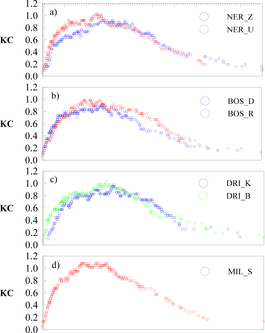
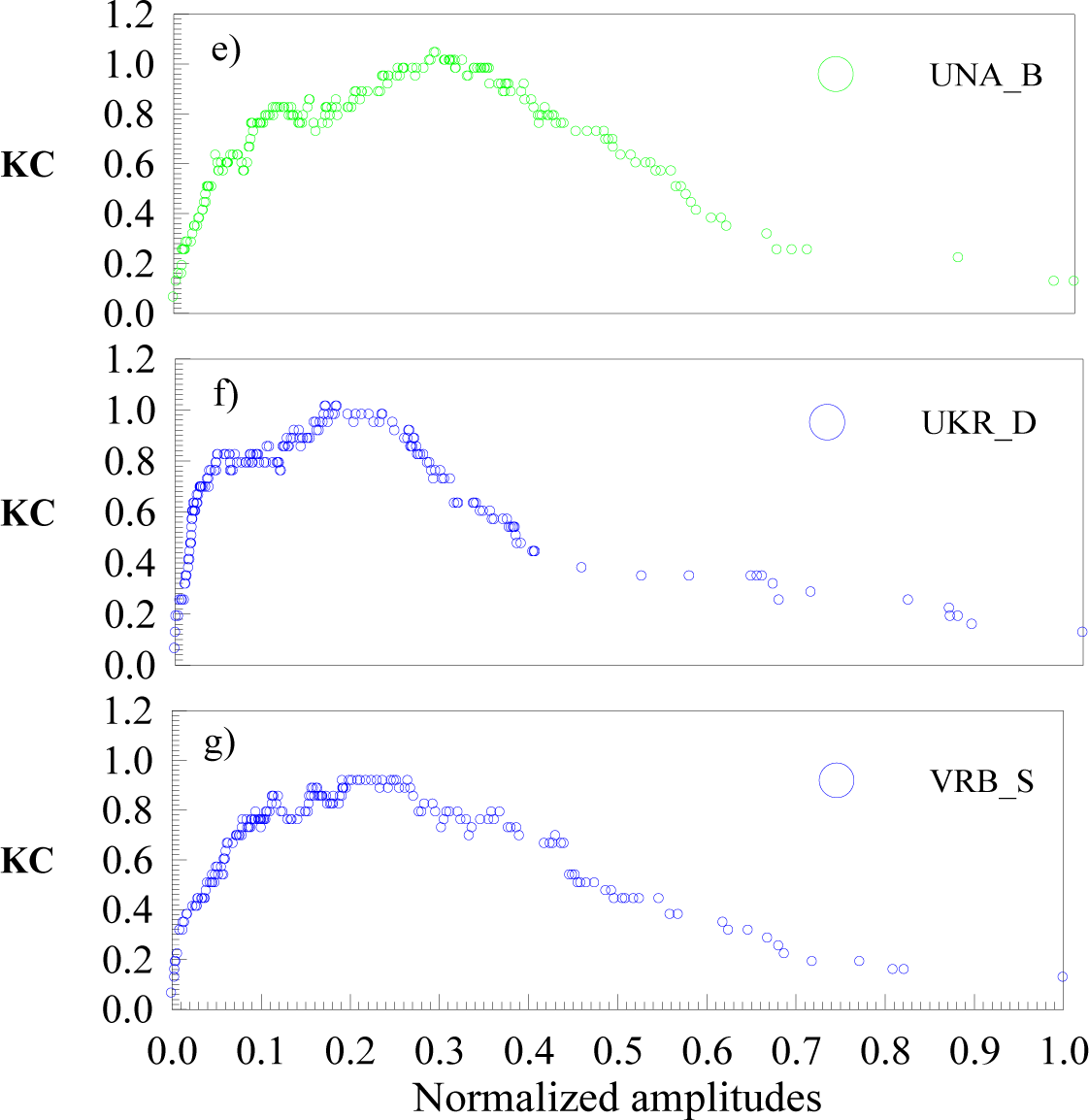
2.2.1. The Kolmogorov Complexity Spectrum

According to Definition 1 in [16], the time series {x_i}, i = 1, 2, 3, …, N is called normalized one (or time series with normalized amplitude) after performing the transformation xi = (X_i− X_min)/(X_max− X_min), where {X_i } is a time series obtained either by a measuring procedure or as an output from a environmental or other model, while X_max = max(X_i) and X_min = min (Xi). From this definition it follows that all elements in time series {x_i} lay in the interval [0, 1]. The Kolmogorov complexity spectrum of time series {x_i} we call the sequence {c_i}, i = 1, 2, 3,…, N obtained by the LZA algorithm which is applied N times on time series, where thresholds {x_t,i} are all elements in {x_i}. Namely, the original time series samples are converted into a set of 0–1 sequences {S(k) i}, i = 1, 2, 3, …, N, k = 1, 2, 3, …, N, defined by comparison with a threshold {x_t,_k}:

$$s_i{}^{(k)}=\{{}_{1,x_i\ge x_{t,k}}^{0,x_i<x_{t,k}}.$$

(4)

After we apply the LZA algorithm on each element of the series {S_i^(k)} we get the KC complexity spectrum {c_i}, i = 1, 2, 3, …, N. This spectrum allows us to explore the range of amplitudes in a time series representing a process, for which it has highly enhanced stochastic components, i.e., highest complexity. The highest value $K_{\max }^C$ in this series, i.e., $K_{\max }^C=\max \left\{c_i\right\}$, we call the Kolmogorov complexity spectrum highest value (KCM).

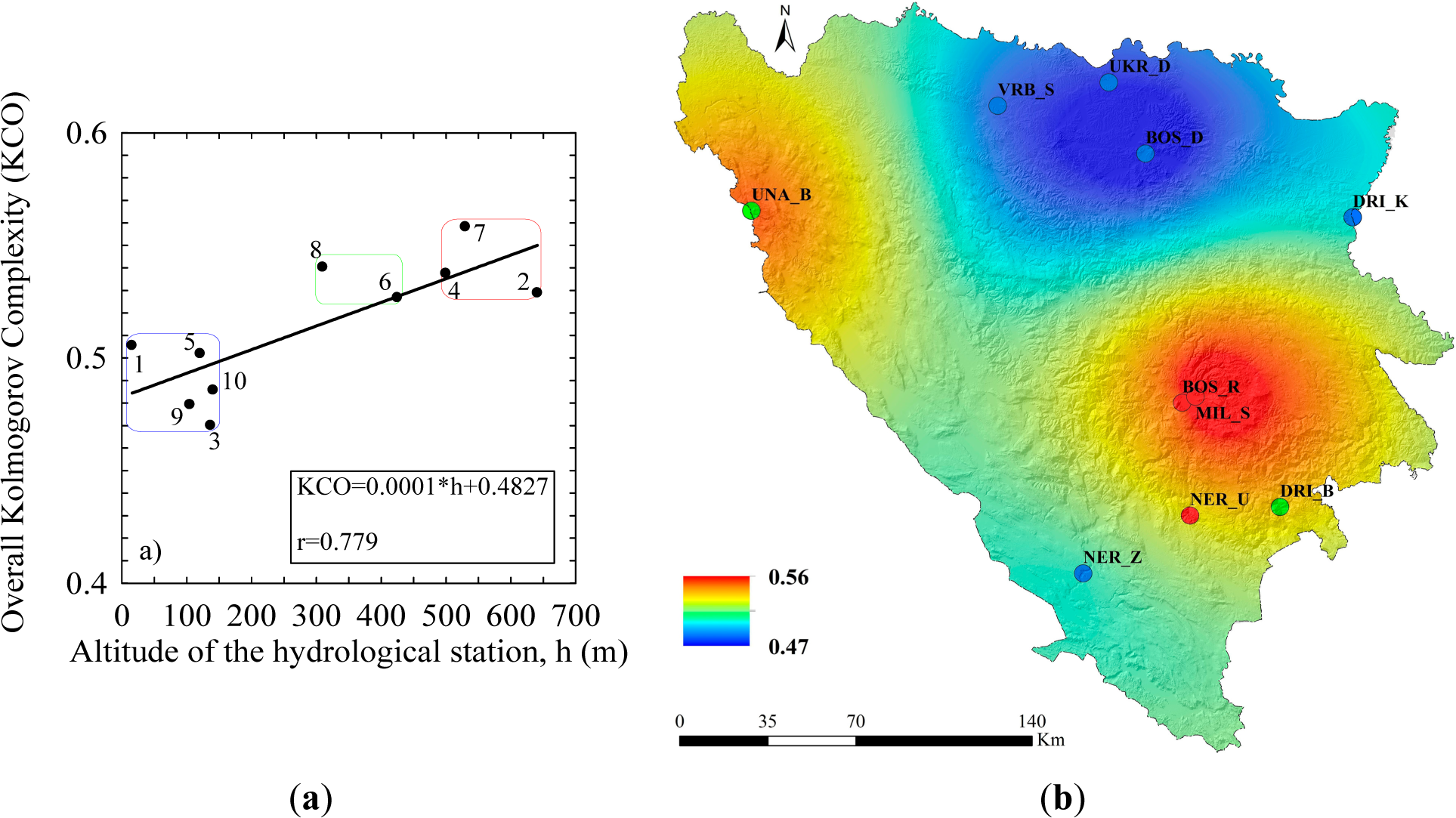
2.2.2. The Overall Kolmogorov Complexity Information Measure

The KC complexity as an information measure cannot distinguish between time series with different amplitude variations and similar random components. This is also true of the suggested KCM measure, although it gives more information about randomness, in a broader context, than the KC one does. When we convert a time series into a string then its complexity is hidden in the coding rules. Thus, neither the KC nor the KCM complexity is able to discern between time series with different Kolmogorov spectra of complexity. From this reason, in the analysis of the river flow time series we use an overall Kolmogorov complexity information measure$K_O^C$ (KCO in further text) which is according to [16] defined as:

$$K_O^C=\frac{1}{x_m}{\displaystyle \underset{X}{\int }{K}_S^{C}dx}$$

(5)

where $K_S^C$ is the spectrum of the Kolmogorov complexity, x_m is a highest value of the physical quantity in a time series, while dx and X are differential and domain of that quantity, over which this integral takes values, respectively. Since $K_S^C$ is given as the sequence $\left\{K_S^C\right\},i=1,2,3,\dots ,N$, it is calculated numerically as:

$$K_C^O=\frac{1}{x_m}\left[K_1^C\left(x_2-x_1\right)+\frac{1}{2}{\displaystyle \sum _{i=1}^{N-1}{K}_i^C\left(x_{i+1}-x_{i-1}\right)+K_N^C\left(x_N-x_{N-1}\right)}\right]$$

(6)

The $K_O^C$ takes value on the interval (0, K_u), where K_u can also takes value larger than 1. This information measure can make distinction between different time series having close values of the KC and KCM.

3. Datasets and Computations

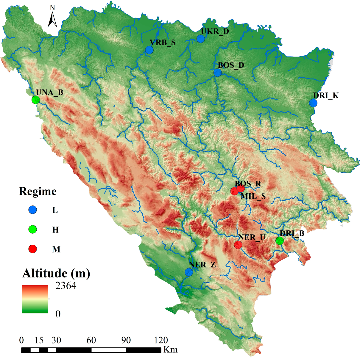
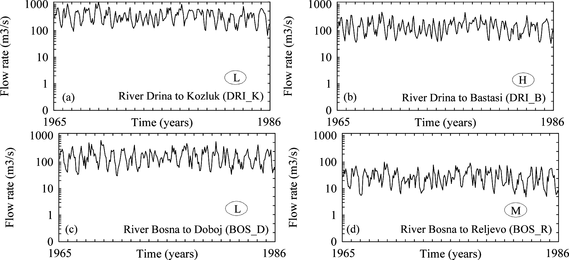
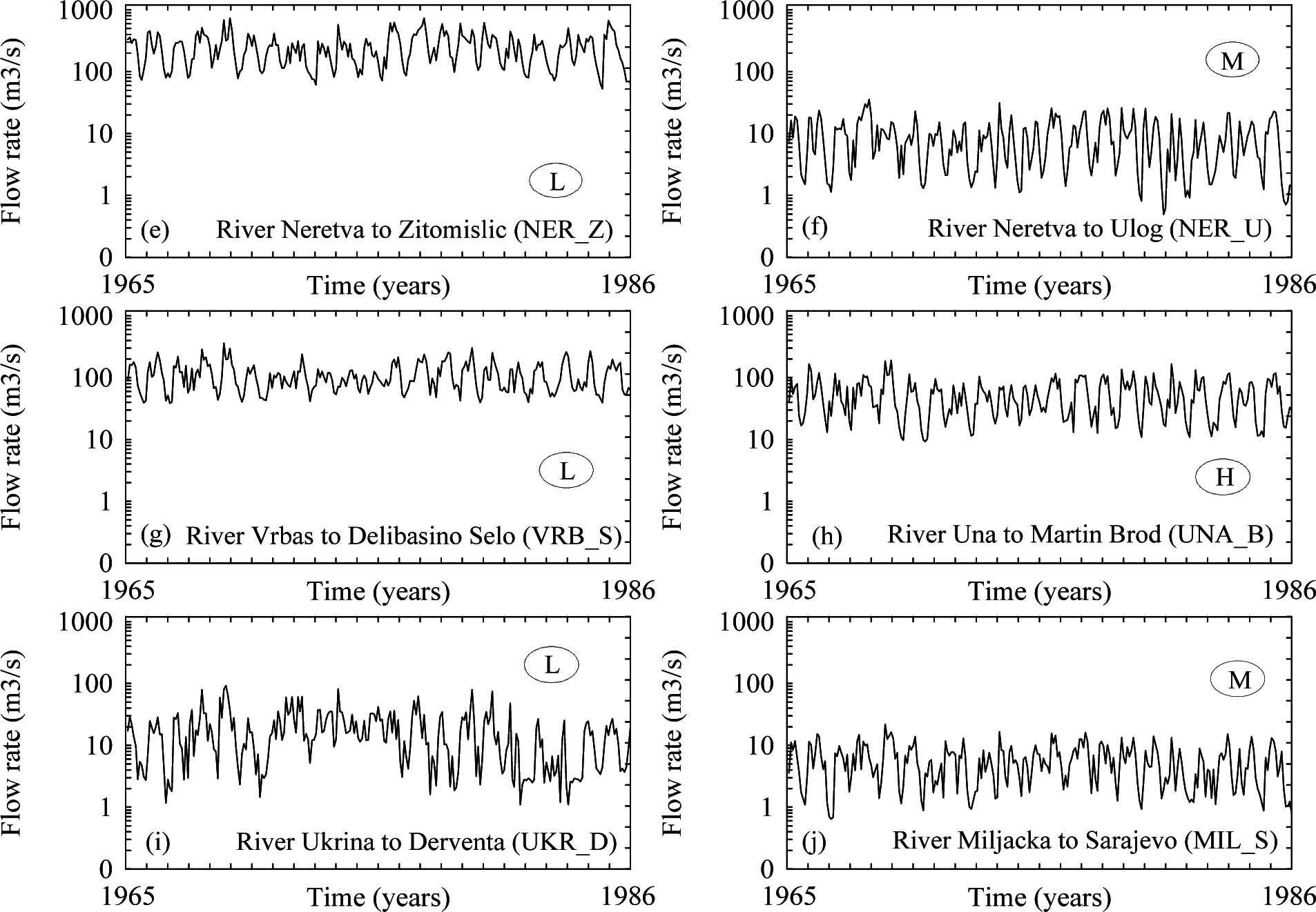
3.1. Short Description of River Locations and Time Series

River flow records in the Bosnia and Herzegovina are, in general, of relatively short duration. Except for several rivers [4], many measurements only began in the late 1950s. For this study we have selected seven rivers located in the territory of Bosnia and Herzegovina, which is in the western Balkans, surrounded by Croatia to the north and south-west, Serbia to the east, and Montenegro to the southeast. It lies between latitudes 42° and 46° N, and longitudes 15° and 20° E. The country is mostly mountainous, encompassing the central Dinaric Alps. The northeastern parts reach into the Pannonian basin, while in the south it borders the Adriatic Sea. Dinaric Alps generally run in east-west direction, and get higher towards the south. The highest point of the country is peak Maglić at 2386 m, at the Montenegrin border, while the major mountains include Kozara, Grmeč, Vlašić, Čvrsnica, Prenj, Romanija, Jahorina, Bjelašnica and Treskavica (Figure 1).

Since the purpose of this paper is to quantify the degree of randomness in the river flow time series of rivers in Bosnia and Herzegovina, in different parts of their courses, we have made a selection of hydrological stations on the basis of classification of typology for mountains and other relief classes according to [27]. This classification can be summarized on the following way: (i) lowlands (0–200 m mean altitude—in further text L type), (ii) platforms and hills (200–500 m—H type) and (iii) mountains with mean elevations between 500 and 6000 m (M type). Thus, we have analyzed: the lower and upper course (the rivers Neretva, Drina and Bosnia), the upper course (the rivers Una and Miljacka) and the lower course (the river Vrbas and Ukrina). These catchments are listed in

Table 1. Rivers in Bosnia and Herzegovina used in the study with the corresponding flow rates (FR—mean; FR_max—maximal; FR_min—minimal for the period 1965–1985) and their classification following a classification of typology for mountains and other relief classes by [27]: lowland (altitude < 200 m)—(L regime), platforms and hills (200 < altitude < 500 m)—(H regime) and mountains (500 < altitude < 6000 m)—(M regime).

Catchment	Number	Abbreviation	Longitude (°E)	Latitude (°N)	Altitude (m)	FR (m3/s)	FRmax(m3/s)	FRmin (m3/s)	Regime
River Neretva to Zitomislić	1	NER_Z	17°47′	43°12′	16	252.0	734.0	53.0	L
River Neretva to Ulog	2	NER_U	18°14′	43°25′	641	8.0	35.3	0.5	M
River Bosna to Doboj	3	BOS_D	18°16′	43°49′	137	172.0	650.0	30.0	L
River Bosna to Reljevo	4	BOS_R	18°06′	44°44′	500	29.0	99.5	4.8	M
River Drina to Kozluk	5	DRI_K	19°07′	44°30′	121	380.0	1160.0	66.0	L
River Drina to Bastasi	6	DRI_B	18°46′	43°27′	425	155.0	497.0	32.7	H
River Miljacka to Sarajevo	7	MIL_S	18°21′	43°12′	530	5.0	21.9	0.6	M
River Una to Martin Brod	8	UNA_B	16°07′	43°30′	310	54.0	188.0	9.2	H
River Ukrina to Derventa	9	UKR_D	17°55′	44°50′	105	17.0	92.3	1.1	L
River Vrbas to Delibašino Selo	10	VRB_S	18°16′	43°49′	141	111.0	358.0	38.2	L

.

They are spread across the country and are representative for catchments in these regions. Datasets of monthly river flow rates for the period 1965–1986 were taken from the Annual Report of the Hydrometeorological Institute of Bosnia and Herzegovina, consisting of 252 data points in each time series.

3.2. Computation of Information Measures for Seven River Flow Time Series

Using the calculation procedure outlined in Sections 2.1 and 2.2, we have computed the KCL, KCU, the Kolmogorov complexity spectrum and the KCO values for the ten river flow time series of seven rivers (Figure 2) in Bosnia and Herzegovina. The calculations are carried out for the entire time interval 1965–1986.

4. Results and Discussion

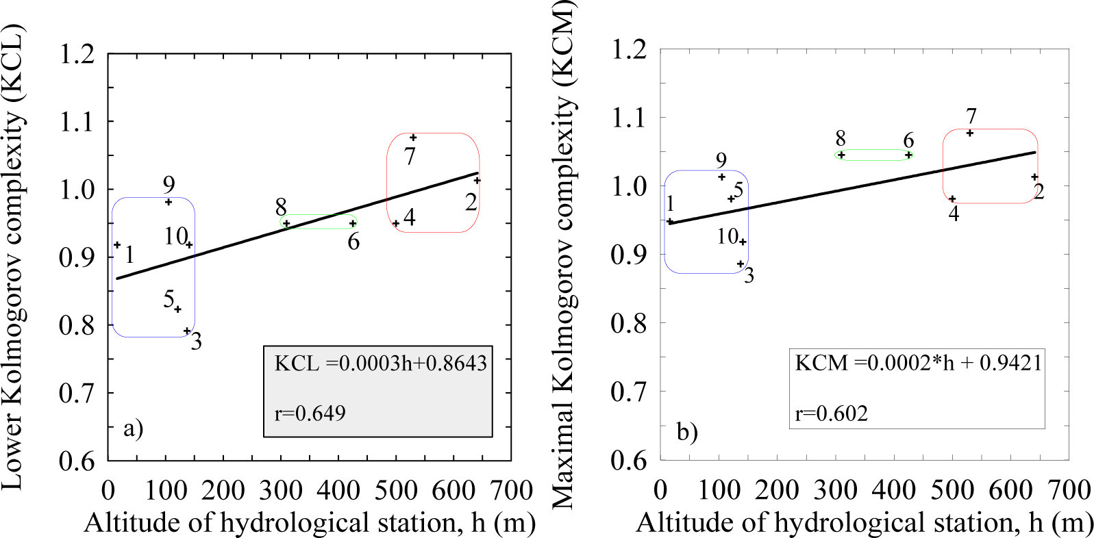
4.1. The Lower (KCL), Upper (KCU) Kolomogorov Complexity and Kolmogorov Complexity Spectrum Highest Value (KCM)

Results for Kolmogorov complexities (lower—KCL, upper—KCU, Kolmogorov complexity spectrum highest value—KCM) and overall Kolmogorov complexity information measure (KCO) are given in the corresponding rows of

Table 2. Kolmogorov complexities (lower—KCL, upper—KCU, Kolmogorov complexity spectrum highest value—KCM) and overall Kolmogorov complexity information measure (KCO) values of the flow rate for ten time series of seven rivers in Bosnia and Herzegovina for the period 1965–1986.

Catchment	Number	Regime	Abb.	KCL	KCU	KCM	KCO
River Neretva to Zitomislić	1	L	NER_Z 0.918 3.799 0.948 0.506
River Neretva to Ulog	2	M	NER_U	1.013	3.309	1.013	0.529
River Bosna to Doboj	3	L	BOS_D	0.791	3.277	0.886	0.470
River Bosna to Reljevo	4	M	BOS_R	0.948	4.092	0.981	0.538
River Drina to Kozluk	5	L	DRI_K	0.823	3.213	0.981	0.502
River Drina to Bastasi	6	H	DRI_B	0.948	3.605	1.045	0.529
River Miljacka to Sarajevo	7	M	MIL_S	1.076	4.194	1.077	0.558
River Una to Martin Brod	8	H	UNA_B	0.948	4.227	1.045	0.540
River Ukrina to Derventa	9	L	UKR_D	0.981	4.294	1.013	0.479
River Vrbas to Delibašino Selo	10	L	VRB_S	0.918	4.324	0.918	0.486

. From this table it is seen that the KCL values for seven rivers can be classified into two intervals, i.e., (0.948, 1.076) and (0.791, 0.918), which corresponds to the upper (H and M regimes) and the lower river course (L regime), respectively.

Note that a least complex process has a KCL value near to zero, whereas a process with the highest randomness will have the KCL close to one. The KCL information measure can be also considered as a measure of randomness. Thus, a value of the KCL near zero is associated with a simple deterministic process like a periodic motion, whereas a value close to one is associated with a stochastic process [3,4]. Accordingly, the KCL values, which are large for rivers from the first interval, i.e., (0.948, 1.076), indicate the presence of stochastic influence in their upper courses, where these rivers show behavior that is typical for mountain rivers. Inversely, the KCL complexities are smaller for the lower river courses (0.791, 0.918). The only exception is the Ukrina River (UKR_D) having greater randomness which is closer to the KCL of mountain rivers (0.981), which could be attributed to the fact that the KCL information measure neglects variability in time series amplitudes. Similar results are observed in analysis of the KCU information measure. However, now except to the river Ukrina River (UKR_D) and the Vrbas River (VRB_S) has the KCU closer to the H and M regimes (4.324).

Figure 3 depicts the changes in the KCL and KCM complexities of river flow rate for ten time series of seven rivers in Bosnia and Herzegovina for the period 1965–1986, in dependence on the altitude of hydrological station. There is a positive trend in changes of the KCL and KCM with coefficients of correlation r, which are close to each other 0.649 and 0.602, respectively.

4.2. The Kolmogorov Complexity Spectrum

Over the last decade many results have been obtained about the chaotic nature of river flow using different techniques like complexity measures [7,8], detrended cross-correlation analysis, formalism of fractal analysis etc., to provide deeper insight regarding this issue [3,28,29]. We have analyzed the monthly river flow time series of the seven rivers in Bosnia and Herzegovina for the period 1965–1986, with N = 252 data points. The curves describing the Kolmogorov complexity spectra for the time series of flow rate of seven rivers and ten stations are depicted in Figure 4. From this figure it is seen that flow dynamics of rivers are different in sense of the position and value of the maximum of the Kolmogorov complexity spectrum highest value (KCM). A simple inspection of this figure indicates the following facts for the same river: (i) when the river is in the M regime, i.e., with a pronounced presence of stochastic components in the river flow, then the KCM is greater in comparison with its KCM in the L regime; (ii) the position of the maximum in the M regime is shifted towards the smaller normalized amplitudes (Figures 4a,b); (iii) when the river is in the H regime, i.e., when presence of stochastic components in the river flow is less pronounced than in M regime, then the KCM is slightly greater in comparison with its KCM in the L regime, while the position of the maximum in the H regime is still shifted towards the smaller values in the spectrum (Figure 4c). Note, that these conclusions could not be obtained if we compare the regimes of different rivers. From other Figures 4d–g it is seen that the maximum of the Kolmogorov complexity spectrum of the river flow time series is more shifted to the smaller values for the regimes where river flow has the higher randomness.

Analysis of Table 2 indicates that the KCM values in seven rivers are classified into two intervals, i.e., (1.013, 1.077) and (0.886, 0.948) corresponding to H and M river regimes and L river regime, respectively, while the UKR_D river is an exception with the KCM value of 1.013.

4.3. The Overall Kolmogorov Complexity Information Measure

The KCL as a measure does not “see” a difference between time series which have different amplitude variations but similar random components. This could also be said for the KCM information measure, although it gives more information about complexity, in a broader context, than the KCL one does. It is seen from the analysis of KCL and KCM rows in Sections 3.2 and 3.3. However, it seems that the KCO information measure better takes into account both, i.e., the amplitude and the place of the components in a time series. A detailed inspection of column KCO in Table 2 and Figure 5a that there exist two intervals of this information measure, which are clearly separated: (1) (0.470, 0.506) and (2) (0.529, 0.558).

The first interval includes KCO of the flow rate of rivers in the L regime while another one refers to the H and M regimes. Now, the complexities of the UKR_D and VRB_S rivers, described by the KCO information measure, correspond to the less stochastic time series. It seems that this is more realistic measure than when their time series are described by the KCL, KCU and KCM information measures.

Figure 5b depicts a spatial distribution of the KCO information measure of flow rate for ten stations of seven rivers for the period 1965–1986. This map enhances two regions: (i) with the higher KCO, which is strongly influenced by the high mountain relief in the northwestern and eastern part of Bosnia and Herzegovina including the H and M river regimes (red color) and (ii) with the lower KCO, which corresponds to the lowland regions (the northern, northeastern, western and southeastern parts with L river regimes (blue color). In the central part of Bosnia and Herzegovina there exists a transition belt with the KCO values indicating to the mixed influences of the relief.

4. Conclusions

In the present study we have analyzed monthly river flow to assess the Kolmogorov complexity based information measures in river flow dynamics using ten time series of seven rivers in Bosnia and Herzegovina for the period 1965–1986. We have examined the monthly river flow time series for seven rivers: (i) the Neretva, the Bosnia and the Drina (in the mountain and lowland parts), (ii) the Miljacka and the Una (in the mountain part) and the Vrbas and the Ukrina (in lowland part) and calculated the KCL, KCU, the Kolmogorov complexity spectrum, KCM and KCO values for each time series. The KCL as an information measure does not “see” a difference between time series, which have different amplitude variations but similar random components. This could also be said for the KCM information measure, although it gives more information about randomness, in a broader context, than the KCL one does. However, it seems that the KCO information measure better takes into account both, i.e., the amplitude and the place of the components in a time series.

Finally, we provide an outlook of potential use of Kolmogorov complexity based information measures in study of the river flow dynamics. The KC information measure calculated by the LZA algorithm has an attractive feature that it is model-independent. It means that it can be applied to both deterministic as well as stochastic processes and does not require the process to be stationary. Therefore, it is often used in the complexity analysis of the river flow dynamics. However, the KC as a measure does not distinguish between time series with different amplitude variations and similar random components. In addition, to calculate this measure we have to convert a time series into a string. When we do that its complexity is hidden in the coding rules. Thus, in the procedure of establishing a threshold for a criterion for coding, some information about the structure of the time series can be lost. With the suggested information measures we: (i) increase the number of information, which we get about the randomness of the river flow and (ii) include the amplitude and the place of the components in the river flow time series. Applications of these information measures may be useful in developing appropriate models of river flow activity and analysis of river flow time series of different regimes.

References

1. Schertzer, D.; Tchiguirinskaia, I.; Lovejoy, S.; Hubert, P.; Bendjoudi, H.; Larchevesque, M. Discussion of “Evidence of chaos in rainfall-runoff process”. Which chaos in rainfall-runoff process? Hydrol. Sci. J 2002, 47, 139–149. [Google Scholar]
2. Salas, J.D.; Kim, H.S.; Eykholt, R.; Burlando, P.; Green, T.R. Aggregation and sampling in deterministic chaos: implications for chaos identification in hydrological processes. Nonlinear Proc. Geoph 2005, 12, 557–567. [Google Scholar]
3. Zunino, L.; Soriano, M.C.; Rosso, O.A. Distinguishing chaotic and stochastic dynamics from time series by using a multiscale symbolic approach. Phys. Rev. E 2012, 86, 046210. [Google Scholar]
4. Mihailović, D.T.; Nikolić-Djorić, E.; Drešković, N.; Mimić, G. Complexity analysis of the turbulent environmental fluid flow time series. Physica A 2014, 395, 96–104. [Google Scholar]
5. Weijs, S.V.; van de Giesen, N.; Parlange, M.B. HydroZIP: How hydrological knowledge can be used to improve compression of hydrological data. Entropy 2013, 15, 1289–1310. [Google Scholar]
6. Weijs, S.V.; van de Giesen, N.; Parlange, M.B. Data compression to define information content of hydrological time series. Hydrol. Earth Syst. Sc 2013, 17, 3171–3187. [Google Scholar]
7. Lange, H.; Rosso, O.A.; Hauhs, M. Ordinal patterns and statistical complexity analysis of daily stream flow time series. Eur. Phys. J. ST 2013, 222, 535–552. [Google Scholar]
8. Serinaldi, F.; Zunino, L.; Rosso, O.A. Complexity—entropy analysis of daily stream flow time series in the continental United States. Stoch. Env. Res. Risk A 2014, 28, 1685–1708. [Google Scholar]
9. Andriani, P.; McKelveyll, B. From Gaussian to Paretian Thinking: Causes and Implications of Power Laws in Organizations. Organ. Sci 2009, 20, 1053–1071. [Google Scholar]
10. Thompson, M.; Young, L. The complexities of measuring complexity. Presented at IMP Conference, Rome, Italy; 2012. Available online: http://www.impgroup.org/uploads/papers/7846.pdf accessed on 7 May 2015.
11. Weisberg, S. Applied Linear Regression, 3rd ed; Wiley: Hoboken, NJ, USA, 2005; p. 305. [Google Scholar]
12. Shalizi, C.R. Estimating Distributions and Densities. Available online: http://www.stat.cmu.edu/~cshalizi/350/lectures/28/lecture-28.pdf accessed on 7 May 2015.
13. Otache, Y.M.; Sadeeq, M.A.; Ahaneku, I.E. ARMA modelling of Benue river flow dynamics: Comparative study of par model. Open J. Modern Hydrol 2011, 1, 1–9. [Google Scholar]
14. Li, M.; Vitanyi, P. An Introduction to Kolmogorov Complexity and its Applications, 2nd ed; Springer: Berlin, Germany, 1997; p. 188. [Google Scholar]
15. Lempel, A.; Ziv, J. On the complexity of finite sequences. IEEE Trans. Inf. Theory 1976, 22, 75–81. [Google Scholar]
16. Mihailović, D.T.; Mimić, G.; Nikolić-Djorić, E.; Arsenić, I. Novel measures based on the Kolmogorov complexity for use in complex system behavior studies and time series analysis. Open Phys 2015, 13, 1–14. [Google Scholar]
17. Feldman, D.P.; Crutchfeld, J.P. Measures of Statistical Complexity: Why? Phys. Lett. A 1998, 238, 244–252. [Google Scholar]
18. Kolmogorov, A. Logical basis for information theory and probability theory. IEEE Trans. Inf. Theory 1968, IT-14, 662–664. [Google Scholar]
19. Cerra, D.; Datcu, M. Algorithmic relative complexity. Entropy 2011, 13, 902–914. [Google Scholar]
20. Kaspar, F.; Schuster, H.G. Easily calculable measure for the complexity of spatiotemporal patterns. Phys. Rev. A 1987, 36, 842–848. [Google Scholar]
21. Zhang, X.S.; Roy, R.J.; Jensen, E.W. EEG complexity as a measure of depth of anesthesia of patients. IEEE Trans. Biomed. Eng 2001, 48, 1424–1433. [Google Scholar]
22. Radhakrishnan, N.; Wilson, J.D.; Loizou, P.C. An alternative partitioning technique to quantify the regularity of complex time series. Int. J. Bifurcation Chaos 2000, 10, 1773–1779. [Google Scholar]
23. Small, M. Applied Nonlinear Time Series Analysis: Applications in Physics, Physiology and Finance; World Scientific: Singapore, Singapore, 2005; p. 245. [Google Scholar]
24. Ferenets, R.; Lipping, T.; Anier, A. Comparison of entropy and complexity measures for the assessment of depth of sedation. IEEE Trans. Biomed. Eng 2006, 53, 1067–1077. [Google Scholar]
25. Hu, J.; Gao, J.; Principe, J.C. Analysis of biomedical signals by the Lempel–Ziv complexity: the effect of finite data size. IEEE Trans. Biomed. Eng 2006, 53, 2606–2609. [Google Scholar]
26. Thai, Q. calc_lz_complexity: Calculates the Lempel-Ziv Complexity of binary sequence—a measure of its “randomness”. Available online: http://www.mathworks.com/matlabcentral/fileexchange/38211-calclzcomplexity accessed on 15 December 2014.
27. Meybeck, M.; Green, P.; Vorosmarty, C. A new typology for mountains and other relief classes: An application to global continental water resources and population distribution. Mt. Res. Dev 2001, 21, 34–45. [Google Scholar]
28. Salas, J.D.; Kim, H.S.; Eykholt, R.; Burlando, P.; Green, T.R. Aggregation and sampling in deterministic chaos: Implications for chaos identification in hydrological processes. Nonlinear Process. Geophys 2005, 12, 557–567. [Google Scholar]
29. Hajian, S.; SadeghMovahed, M. Multifractal detrended cross-correlation analysis of sunspot numbers and river flow fluctuations. Physica A 2010, 389, 4942–4957. [Google Scholar]
Figure 1. Relief of Bosnia and Herzegovina with the location of the ten hydrological stations on seven rivers used in the study (the abbreviations for rivers and letters indicating the river regime are given in Table 1).
Entropy 17 02973f1
Figure 2. Ten river flow time series of seven rivers in Bosnia and Herzegovina for the period 1965–1986.
Entropy 17 02973f2aEntropy 17 02973f2b
Figure 3. The dependence of KCL and KCM complexities of river flow rate on altitude, for ten time series of the seven rivers in Bosnia and Herzegovina for the period 1965–1986. Closed contours indicate the river regime: L (blue), H (green) and M (red).
Entropy 17 02973f3
Figure 4. The Kolmogorov complexity spectra for the normalized amplitude of the monthly flow rate time series of the seven rivers in Bosnia and Herzegovina for the period 1965–1986. The circles indicate the regime of river course: L (blue), H (green) and M (red).
Entropy 17 02973f4aEntropy 17 02973f4b
Figure 5. The KCO information measure: Dependence on altitude (a) and spatial distribution (b) of the monthly flow rate for ten time series of seven rivers in Bosnia and Herzegovina for the period 1965–1986.
Entropy 17 02973f5