General Hyperplane Prior Distributions Based on Geometric Invariances for Bayesian Multivariate Linear Regression

Abstract

Based on geometric invariance properties, we derive an explicit prior distribution for the parameters of multivariate linear regression problems in the absence of further prior information. The problem is formulated as a rotationally-invariant distribution of L-dimensional hyperplanes in N dimensions, and the associated system of partial differential equations is solved. The derived prior distribution generalizes the already known special cases, e.g., 2D plane in three dimensions.

1. Introduction

In the context of Bayesian probability theory, a proper assignment of prior probabilities is crucial. Depending on the domain, quite different prior information can be available. It may be in the form of point estimates provided by domain experts (see, e.g., [1] for prior distribution elicitation) or in the form of invariances (of the prior knowledge) of the system of interest, which should be reflected in the prior probability density [2]. However, especially for the ubiquitous case of the estimation of parameters of linear equation systems (like a straight line or hyperplane fitting), the latter requirement is often violated. Consider, for concreteness, the simple case of y = ax, a straight line through the origin, with a the parameter of interest. Here, the commonly-applied prior is constant, p (a|I) = const., often accompanied by statements like “Since we do not have specific prior information, we chose a uniform prior on a…”. 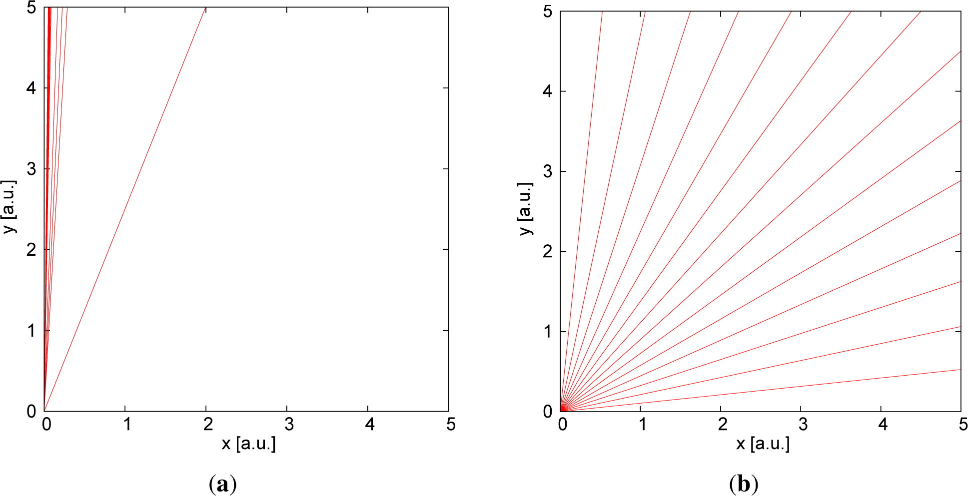In Figure 1 on the left-hand side, 15 random samples generated from this prior distribution with a ∈ [0, 50] are displayed. Confronted with this result, the typical response is (at least in the experience of the author) that instead, a more “uniform” prior distribution of the slopes was intended, which is often depicted like in Figure 1 on the right-hand side. This plot was generated from a prior distribution that has an equal probability density for the angle of the line to the abscissa, corresponding to

$$p(a|I)~\frac{1}{{\left(1+a^2\right)}^{3/2}}.$$

(1)

Additionally, in fact, in practice, the units of the axes are commonly chosen in such a way that extreme values of the slopes are not a priori overrepresented. If we generalize this requirement to more than one independent or dependent variable, then the desired prior probability should be invariant under arbitrary rotations in this parameter space. Some important special cases have been given already in [3], e.g., for a 1D line in two dimensions or a 2D plane in three dimensions. There also, the governing transformation invariance equation underlying invariant priors is derived. These special cases have since then been generalized to invariant priors for (N − 1)-dimensional hyperplanes in N-dimensional space; see, e.g., [4]. These hyperplane priors proved to be valuable for Bayesian neural networks [5], where the specific properties of the prior density favored node-pruning instead of simple edge pruning of standard (quadratic) weight regularizers. This is especially helpful for a Bayesian approach to fully-connected deep convolutional networks; see e.g., [6,7].

Nevertheless, the general case of prior probability densities for L-dimensional hyperplanes in N-dimensions (N > L) in a suitable parameterization has not been available so far. It has even been conjectured that it is impossible to derive a general solution [8]. Luckily, this conjecture has been too pessimistic, and an explicit formula for the prior density, which can directly be applied to linear regression problems, is derived below.

It should be pointed out that multivariate regression is of course a longstanding topic in Bayesian inference. with classical contributions, e.g., by Box and Tiao [9], Zellner [10] or West [11]. However, the standard approach is based on the use of conjugate priors (instead of invariance priors), mostly for computational convenience [12]. In contrast, the subsequently derived prior distribution is determined by the basic desideratum of consistency if the available prior information is invariant under the considered transformations (i.e., rotations). Whether this invariance holds depends on the considered problem and must not be assumed without further consideration (similar to the case of flat priors for the coefficients). For example, the assumption of rotation invariance may not be suitable for covariates with different underlying units (e.g., m², kg).

2. Problem Statement

In standard notation, a multivariate regression model is notated as follows:

$${\mathbf{y}}_i={\mathbf{A}}_{{\mathbf{X}}_i}+\mathbf{t},x_i\in {ℝ}^L,\mathbf{A}\in {ℝ}^{M\times L},\mathbf{t}\in {ℝ}^M\text{and}{y}_i\in {ℝ}^M,$$

(2)

with:

$${\mathbf{z}}_i={\mathbf{y}}_i+{ϵ}_i,{ϵ}_i\in {ℝ}^M,$$

(3)

where z_i is the response vector, y_i the model value vector, x_i the vector of the L covariates for observation i, t the intercept vector and A the M × L-dimensional matrix of adjacent regression coefficients. The observation noise ϵ_i of each data point is often considered as Gaussian distributed, ${ϵ}_i~\text{N(0,}\sum \text{)}$. This regression model can also be considered as estimating the “best” L-dimensional hyperplane in an N-dimensional space, because in an N-dimensional space, an L-dimensional hyperplane is given by:

$$\begin{array}{c}{y}_1=a_{11}{x}_1+a_{12}{x}_2+\cdots +a_{1L}{x}_L+t_1\\ y_2=a_{21}{x}_1+a_{22}{x}_2+\cdots +a_{2L}{x}_L+t_2\\ y_3=a_{31}{x}_1+a_{32}{x}_2+\cdots +a_{3L}{x}_L+t_3\\ ⋮\\ y_M=a_{M1}{x}_1+a_{M2}{x}_2+\cdots +a_{ML}{x}_L+t_M\end{array}$$

(4)

with M = N − L.

The quantity of interest is the prior probability density F (A) = F (a₁₁, ⋯, a_ML, t₁, ⋯, t_M|I) for the coefficients a₁₁, ⋯, a_ML, t₁, ⋯, t_M, which remains invariant under translations and rotations of the coordinate system.

3. Derivation

Using the transformation invariance equation derived in [3]:

$${\displaystyle \sum _{i=1}^N\frac{\partial }{{\partial }_{z_i}}(F(z_1,\cdots ,z_N)g_i(z_1,\cdots z_N))}=0$$

(5)

for infinitesimal transformations of the form ${z^{\prime }}_i=z_i+ϵg_i(z_1,\cdots z_N)$, we can establish a partial differential equation system for F.

3.1. Invariance under Translations

Let us first consider a translation with respect to $y_i:{y^{\prime }}_i=y_i+ϵ$, i.e., g_i = 1, g_j,j≠i = 0. Then, the equation in the primed variables reads:

$${y^{\prime }}_i=y_i+ϵ={a^{\prime }}_{i1}{x}_1+{a^{\prime }}_{i2}{x}_2+\cdots +{a^{\prime }}_{iL}{x}_L+{t^{\prime }}_i$$

(6)

Collecting the coefficients yields ${t^{\prime }}_i=t_i+ϵ$, and therefore, Equation (5) results in:

$$0+\cdots +0+\frac{\partial }{\partial t_i}(F(\mathbf{A},\mathbf{t})\cdot 1)+0+\cdots +0=0,$$

(7)

which holds for any i. Therefore, F (A, t) can be a function of $\overrightarrow{a}$ only. Since F (A|I) does not depend on $\overrightarrow{t}$, the prior distribution is improper (not normalizable in t) as long as there are no limits on the magnitude of t.

The translation with respect to x_i results in the same conclusion.

3.2. Invariance under Rotations

The general rotation in n-dimensional space may be expressed as a sequence of rotations around rotation axes, which are perpendicular to the planes spanned by appropriately-chosen pairs of coordinate system basis vectors [13]. This is based on the fact that any orthogonal matrix, i.e., rotation matrices, can be written uniquely as a product of 2 × 2 rotations. To avoid convoluted language, we denote in the following the rotation around the rotation axis that is perpendicular to the plane spanned by the linear combination of the basis vectors e_i and e_j simply as rotation in the x_ix_j-plane.

3.2.1. Rotation in the x_ix_j-Plane

Now, we perform one such infinitesimal 2 × 2-rotation for independent parameters around an arbitrary rotation axis perpendicular to the plane spanned by e_i and e_j, preserving all other coordinates: ${x^{\prime }}_k=x_k\forall k\ne (j,i)$ and

$${x^{\prime }}_i=x_i-ϵx_j,$$

(8)

$${x^{\prime }}_j=ϵx_i-x_j.$$

(9)

Substituting the primed coordinates into Equation (5) yields the implied transformations:

$${a^{\prime }}_{ki}=a_{ki}-a_{kj}ϵ,$$

(10)

$${a^{\prime }}_{kj}=a_{kj}-a_{ki}ϵ,$$

(11)

$${t^{\prime }}_k=t_k$$

(12)

and, therefore, the partial differential equation:

$${\displaystyle \sum _{k=1}^M\frac{\partial }{\partial a_{ki}}(F(\mathbf{A})\cdot (-a_{kj}))}+{\displaystyle \sum _{k=1}^M\frac{\partial }{\partial a_{kj}}(F(\mathbf{A})\cdot (a_{ki}))=0.}$$

(13)

3.2.2. Rotation in the y_iy_j-Plane

Now, we perform one such rotation in the plane of two dependent parameters e_i and e_j; thus ${y^{\prime }}_k=y_k\forall k\ne (j,i)$ and:

$${y^{\prime }}_i=y_i-ϵy_j,$$

(14)

$${y^{\prime }}_j=ϵy_i-y_j.$$

(15)

Substituting the primed coordinates into Equation (5) yields the implied transformations:

$${a^{\prime }}_{ik}=a_{ik}-a_{jk}ϵ,$$

(16)

$${a^{\prime }}_{jk}=a_{jk}+a_{ik}ϵ,$$

(17)

$${t^{\prime }}_i=t_i-t_jϵ,$$

(18)

$${t^{\prime }}_j=t_j-t_iϵ,$$

(19)

$${t^{\prime }}_k=t_k$$

(20)

and, therefore, the partial differential equation:

$${\displaystyle \sum _{k=1}^M\frac{\partial }{\partial a_{ik}}(F(\mathbf{A})\cdot (-a_{jk}))}+{\displaystyle \sum _{k=1}^M\frac{\partial }{\partial a_{jk}}(F(\mathbf{A})\cdot (a_{ik}))=0.}$$

(21)

3.2.3. Rotation in a Plane Spanned by x_iy_j-Axes

Performing a rotation in the xy-plane, we obtain:

$${x^{\prime }}_i=x_i-ϵy_j,$$

(22)

$${y^{\prime }}_j=ϵx_i+y_j.$$

(23)

which yields (see the Appendix):

$${a^{\prime }}_{ji}=a_{ji}+(1+a_{ji}^2)ϵ,$$

(24)

$${a^{\prime }}_{kl}=a_{kl}+(a_{jl}{a}_{ki})ϵ,$$

(25)

$${t^{\prime }}_k=t_k+(a_{ki}{t}_j)ϵ$$

(26)

and therefore:

$${\displaystyle \sum _{k=1}^M{\displaystyle \sum _{l=1}^L\frac{\partial }{\partial a_{kl}}(F}\cdot (a_{jl}{a}_{ki}))}+\frac{\partial }{\partial a_{kl}}F+F\cdot a_{ji}=0.$$

(27)

4. The PDE System

The translation invariance of Equation (5) excludes a dependence of F on t₁, ⋯, t_M, so F is of the form F(a₁₁, ⋯, a_ML|I). Rotation invariance with respect to the y-axis requires F to fulfill the homogeneous, linear system of first order partial differential equations (i, j ∈ [1, M], i ≠ j) (i.e., Equation (21)):

$${\displaystyle \sum _{k=1}^L\frac{\partial }{\partial a_{jk}}(F\cdot a_{ik})}-{\displaystyle \sum _{k=1}^L\frac{\partial }{\partial a_{ik}}(F\cdot a_{jk})}=0$$

(28)

and similar for rotations around the x-axis (i, j ∈ [1, L], i ≠ j) (Equation (13)):

$${\displaystyle \sum _{k=1}^L\frac{\partial }{\partial a_{kj}}(F\cdot a_{ki})}-{\displaystyle \sum _{k=1}^M\frac{\partial }{\partial a_{ki}}(F\cdot a_{kj})}=0.$$

(29)

Rotations around an axis perpendicular to a plane given by an x,y-pair require the probability distribution to obey also (i ∈ [1, L], j ∈ [1, M]):

$${\displaystyle \sum _{k=1}^M{\displaystyle \sum _{l=1}^L\frac{\partial }{\partial a_{kl}}(F}\cdot (a_{jl}{a}_{ki}))}+\frac{\partial }{\partial a_{ji}}F+F\cdot a_{ji}=0.$$

(30)

Using the product rule, the double sum can be rewritten as

$${\displaystyle \sum _{k=1}^M{\displaystyle \sum _{l=1}^L\frac{\partial }{\partial a_{kl}}(F}\cdot (a_{jl}{a}_{ki}))}={\displaystyle \sum _{k=1}^M{\displaystyle \sum _{l=1}^L{a}_{jl}{a}_{ki}\frac{\partial }{\partial a_{kl}}}F+F\cdot }{\displaystyle \sum _{k=1}^M{\displaystyle \sum _{l=1}^L\frac{\partial }{\partial a_{kl}}}(a_{jl}{a}_{ki})}$$

(31)

and the last term of the previous equation can be split into three parts and simplified:

$$\begin{array}{l}F\cdot {\displaystyle \sum _{k=1}^M{\displaystyle \sum _{l=1}^L\frac{\partial }{\partial a_{kl}}(a_{jl}{a}_{ki})}}=\\ F\cdot {\displaystyle \sum _{k=1,k\ne j}^M\frac{\partial }{\partial a_{ki}}(a_{ji}{a}_{ki})+F\cdot }{\displaystyle \sum _{l=1,l\ne i}^M\frac{\partial }{\partial a_{jl}}(a_{jl}{a}_{ji})+F\cdot }\frac{\partial }{\partial a_{ji}}{a}_{ji}^2=\\ (M-1)a_{ji}F+(L-1)a_{ji}F+2a_{ji}F=(M+L)a_{ji}F.\end{array}$$

(32)

Using this, Equation (30) can be written as:

$${\displaystyle \sum _{k=1}^M{\displaystyle \sum _{l=1}^L{a}_{jl}{a}_{ki}\frac{\partial }{\partial a_{kl}}F}}+\frac{\partial }{\partial a_{ji}}F+(M+L+1)a_{ji}F=0.$$

(33)

5. Solution

This system of PDEs (Equations (28), (29) and (33)) can be tackled with the theory of Lie groups, which provides a systematic, though algebraically-intensive solution strategy, which is implemented in contemporary computer algebra systems. The solutions of several test cases computed by the Maple computer algebra system ( http://www.maplesoft.com/) (it proved to be superior to MATHEMATICA ( www.http://www.wolfram.com/mathematica/) for the present PDE-systems) led to the conjecture that a general solution to this PDE system is given by the sum of the squares of all possible minors of the coefficient matrix:

$$\begin{array}{l}F(a_{11},\cdots ,a_{ML}|I)\\ ={\left[1+{\displaystyle \sum _{k=1}^{\begin{array}{cc}{(}_P^M)& {(}_P^L)\end{array}}{(\det (A^{P,k}))}^2+}{\displaystyle \sum _{k=1}^{\begin{array}{cc}{(}_{P-1}^M)& {(}_{P-1}^L)\end{array}}{(\det (A^{P-1,k}))}^2+\cdots +{\displaystyle \sum _{k=1}^{\begin{array}{cc}{(}_1^M)& {(}_1^L)\end{array}}{(\det (A^{1,k}))}^2}}\right]}^{-\frac{M+L+1}{2}}\end{array}$$

(34)

where Aⁿ denotes a submatrix (minor) of size n × n (this notation is used at various places throughout the paper and should not be confused with the power of a matrix, which does not occur in this paper) and P = Min (M, L). Equation (34) does not appear unreasonable from the onset as prior density, because it preserves the underlying symmetry of the problem (permutation invariance of the parameters) and it is non-negative.

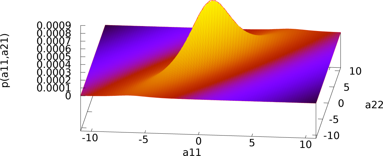
An explicit example for the case N = 4, L = 2 is:

$$F(a_{11},a_{12},a_{21},a_{22},|I)={[1+a_{11}^2+a_{12}^2+a_{21}^2+a_{22}^2+{(a_{11}\cdot a_{22}-a_{12}\cdot a_{21})}^2]}^{-5/2}.$$

(35)

A two-dimensional slice of this probability density is given in Figure 2. The high symmetry of the prior distribution with respect to parameter permutations results in similar, “Cauchy”-like shapes if slices along other parameter axis are displayed.

For the case N = 6, L = 3, the solution is given by:

$$\begin{array}{l}F(a_{11},\cdots ,a_{33}|I)\\ =(1+a_{11}^2+a_{12}^2+a_{13}^2+a_{21}^2+a_{22}^2+a_{23}^2+a_{31}^2+a_{32}^2+a_{33}^2)+\\ {(a_{22}{a}_{33}-a_{23}{a}_{32})}^2+{(a_{21}{a}_{33}-a_{23}{a}_{31})}^2+{(a_{21}{a}_{32}-a_{22}{a}_{31})}^2+\\ {(a_{12}{a}_{33}-a_{13}{a}_{32})}^2+{(a_{11}{a}_{33}-a_{13}{a}_{31})}^2+{(a_{11}{a}_{32}-a_{12}{a}_{31})}^2+\\ {(a_{12}{a}_{23}-a_{13}{a}_{22})}^2+{(a_{11}{a}_{23}-a_{13}{a}_{21})}^2+{(a_{11}{a}_{22}-a_{12}{a}_{21})}^2+\\ {{(a_{11}\cdot (a_{22}{a}_{33}-a_{23}{a}_{32})-a_{12}\cdot (a_{21}{a}_{23}-a_{23}{a}_{31})+a_{13}\cdot (a_{21}{a}_{32}-a_{22}{a}_{31}))}^2)}^{-7/2}.\end{array}$$

6. Proof

6.1. Preliminaries

To prove that Equation (34) fulfills the equation system given by Equations (28), (29) and (33), we verify directly that Equation (34) solves the PDEs.

We will make repeated use of the Laplace expansion of determinants:

$$\det (A^n)={\displaystyle \sum _{j=1}^n{a}_{ij}{(-1)}^{i+j}\det (M_{ij}^{n-1})}$$

(36)

where the minor $M_{ij}^{n-1}$ is the (n − 1) × (n − 1)-matrix derived from the n × n-matrix Aⁿ by deletion of the i-th row and j-th column (by definition M⁰ := 1). The cofactor matrix $A_{ij}^{n-1}$ is defined to be:

$$A_{ij}^{n-1}={(-1)}^{i+j}{M}_{ij}^{n-1}$$

(37)

and satisfies the following n-equations (i, j, k = 1, 2, ⋯, N):

$${\displaystyle \sum _{j=1}^n{a}_{ij}\det (A_{kj}^{n-1})}={\delta }_{ik}\det (A^n),{\displaystyle \sum _{i=1}^n{a}_{ij}\det (A_{ik}^{n-1})}={\delta }_{jk}\det (A^n).$$

(38)

Further useful is the following form of the Laplace expansion, taking into account index shifts of a previous deletion of row k and column i of an (n + 1)-matrix Aⁿ⁺¹, resulting in the minor $M_{ki}^n$:

$$\det (M_{ki}^n)={\displaystyle \sum _{l=1,l\ne i}^{n+1}{a}_{jl}{(-1)}^{(l^{\prime }+j^{\prime })}}\det (M_{(jk)(li)}^{n-1})$$

(39)

where $M_{(jk)(li)}^{n-1}$ is the minor given by deletion of the j-th and k-th row and the l-th and i-th column. l′ and j′ are defined as:

$$\begin{array}{l}{l}^{\prime }=l\forall (l<i)\text{and}{l}^{\prime }=l-1\forall (l>i)\\ j^{\prime }=j\forall (j<k)\text{and}{j}^{\prime }=j-1\forall (j>k).\end{array}$$

(40)

In the following, we face the problem of possibly too heavy of a nomenclature, because we need summation indices, while we also need to keep track of the original indices underlying the entries in the minors, where some rows and columns have been deleted, although the relative order is preserved. The mapping could be expressed, e.g., as $a_{i(i^{\prime })j(j^{\prime })}$ with i′, j′ ∈ [1, m] and i (:) ∈ [1, M] and j (:) ∈ [1, L]. To avoid this cumbersome notation, we implicitly assume from now on (up to the Conclusion Section) this mapping for all summations that are indexed by either k or l. Therefore:

$${\displaystyle \sum _{k=1}^m{a}_{ki}\det (A_{kj}^{m-1})}\text{has to be read as}{\displaystyle \sum _{k^{\prime }=1}^m{a}_{k(k^{\prime })i}\det (A_{k(k^{\prime })j}^{m-1})}.$$

(41)

6.2. x_ix_j- and y_iy_j-Rotations

We now verify that Equation (34) solves Equation (29). It is obvious that only those determinants of Equation (34) that contain column i or column j have the potential to provide non-zero contributions in Equation (29): if column j is missing, the derivative in the first term is zero. If, instead, column i is missing, then the derivative in the second term of Equation (29) yields zero. To proceed, we introduce H(A) via:

$$F(\mathbf{A})=H{(\mathbf{A})}^{-\frac{L+M+1}{2}}.$$

(42)

It is noteworthy that H(A) has a very simple form: it is given by a sum of positive terms. This almost decouples the problem, and we can largely proceed on a term-by-term basis. Using the equality:

$$\frac{\partial }{\partial a_{pq}}{(\det (A^m))}^2=2\det (A^m)\det (A_{pq}^{m-1})$$

(43)

the left-hand side of Equation (29) transforms to (i, j ∈ [1, L], i ≠ j):

$$-(M+L+1)H{(a)}^{-\frac{L+M+3}{2}}\det (A^m).\left({\displaystyle \sum _{k=1}^m{a}_{ki}}\det (A_{kj}^{m-1})-{\displaystyle \sum _{k=1}^m{a}_{kj}}\det (A_{ki}^{m-1})\right)$$

(44)

and using Equation (38), we obtain:

$$-(M+L+1)H{(a)}^{-\frac{L+M+3}{2}}\det (A^m)\cdot ({\delta }_{ij}\det (A^m)-{\delta }_{ij}\det (A^m))=0$$

(45)

and, therefore, Equation (34) solves Equation (29). The calculation is similar for Equation (28) and yields the result that Equation (34) solves also the system Equation (28).

6.3. (x_iy_j)-Rotations

The verification of the successful solution of Equation (33) by Equation (34) requires some more steps. As before, Equation (33) can be written as:

$$-\frac{M+L+1}{2}\left({\displaystyle \sum _{k=1}^M{\displaystyle \sum _{l=1}^L{a}_{jl}{a}_{ki}}H{(\mathbf{A})}^{-\frac{L+M+3}{2}}\frac{\partial H(\mathbf{A})}{\partial a_{kl}}+H{(\mathbf{A})}^{-\frac{L+M+3}{2}}\frac{\partial H(\mathbf{A})}{\partial a_{ji}}-2a_{ji}H{(\mathbf{A})}^{-\frac{L+M+1}{2}}}\right)=0$$

(46)

and after multiplication with $H{(\mathbf{A})}^{\frac{L+M+3}{2}}$ as:

$$\begin{array}{l}-(M+L+1)\cdot \\ \left({\displaystyle \sum _{m=1}^P{\displaystyle \sum _{r=1}^{\begin{array}{cc}{(}_m^M)& {(}_m^L)\end{array}}\left({\displaystyle \sum _{k=1}^m{\displaystyle \sum _{l=1}^m{a}_{jl}{a}_{ki}\det (A^{m,r})\det (A_{kl}^{m-1,r})+\det (A^{m,r})\det (A_{ji}^{m-1,r})}}\right)}}-a_{ji}H(\mathbf{A})\right)\\ =0\end{array}$$

(47)

6.3.1. Matrices with Either Row j or Column i

The inner double sum can be simplified for all matrices containing either row j or column i (i.e., all matrices of size P × P and all matrices A^m,r of size m × m, m ∈ (1, 2, ⋯, P − 1) with label $r=1,2,\cdots ,\left(\begin{array}{c}M\\ m\end{array}\right)\left(\begin{array}{c}L\\ m\end{array}\right)-\left(\begin{array}{c}M-1\\ m\end{array}\right)\left(\begin{array}{c}L-1\\ m\end{array}\right)$ using the Laplace expansion (here, the expansion with respect to row j is shown):

$$\begin{array}{l}{\displaystyle \sum _{k=1}^m{\displaystyle \sum _{l=1}^m{a}_{jl}{a}_{ki}\det (A^{m,r})\det (A_{kl}^{m-1,r})}}\\ =\det (A^{m,r}){\displaystyle \sum _{k=1}^m{a}_{ki}}{\displaystyle \sum _{l=1}^m{a}_{jl}}\det (A_{kl}^{m-1,r})\\ =\det (A^{m,r}){\displaystyle \sum _{k=1}^m{a}_{ki}{\delta }_{jk}\det (A^{m,r})=a_{ji}{(\det (Am,r))}^2}\end{array}$$

(48)

which cancels the corresponding determinant of H (A) in the last term of Equation (48).

6.3.2. Matrices with Neither Row j nor Column i

The basic idea is to show that $\left(\begin{array}{c}M-1\\ m\end{array}\right)\left(\begin{array}{c}L-1\\ m\end{array}\right)$ -matrices with neither row j nor column i, m ∈ (1, 2, ⋯, P − 1), cancel with the contributions of the corresponding matrices including row j and column i of size (m + 1) × (m + 1) of the second term.

Please note that there is a one-to-one correspondence of minors of size m × m without the j-th row and i-th column and the matrices of size (m + 1) × (m + 1) with row j and column i in the second term, therefore allowing one to label both with the same index r. After division by − (M + L + 1), the remaining terms of Equation (48) are (taking into account that the labeling of the rows and columns of the matrices of size (m + 1) × (m + 1) and (m) × (m) must be consistent):

$${\displaystyle \sum _{k=1,k\ne j}^{m+1}{\displaystyle \sum _{l=1,l\ne i}^{m+1}{a}_{jl}{a}_{ki}\det \left(A_{ji}^{m,r}\right)\det \left(A_{(jk)(il)}^{m-1,r}\right)+\det (A^{m+1,r})}\det \left(A_{ji}^{m,r}\right)-a_{ji}{H}_{ji}(\mathbf{A})=0}$$

(49)

with H_ji now only containing determinants with neither row j nor column i. If we now only consider the relevant term of H_ji, we can write:

$${\displaystyle \sum _{k=1,k\ne j}^{m+1}{\displaystyle \sum _{l=1,l\ne i}^{m+1}{a}_{jl}{a}_{ki}\det \left(A_{ji}^{m,r}\right)\det \left(A_{(jk)(il)}^{m-1,r}\right)+\det (A^{m+1,r})}\det \left(A_{ji}^{m,r}\right)-a_{ji}\det {\left(A_{ji}^{m,r}\right)}^2=0}.$$

(50)

The equation is trivially true if det $\left(A_{ji}^{m,r}\right)=0$; otherwise, we can divide by det $\left(A_{ji}^{m,r}\right)$ and obtain:

$${\displaystyle \sum _{k=1,k\ne j}^{m+1}{\displaystyle \sum _{l=1,l\ne i}^{m+1}{a}_{jl}{a}_{ki}\det \left(A_{(jk)(il)}^{m-1,r}\right)+\det (A^{m+1,r})}-a_{ji}\det {\left(A_{ji}^{m,r}\right)}^2=0}.$$

(51)

Replacing the various cofactors by the corresponding minors (cf. Equation (36) and (37)) yields:

$${\displaystyle \sum _{k=1,k\ne j}^{m+1}{\displaystyle \sum _{l=1,l\ne i}^{m+1}{a}_{jl}{a}_{ki}{(-1)}^{(i+j+k^{\prime }+l^{\prime })}\det \left(M_{(jk)(il)}^{m-1,r}\right)+\det (A^{m+1,r})}-a_{ji}{(-1)}^{(i+j)}\det \left(M_{ji}^{m,r}\right)=0}$$

(52)

and after replacing det (A^m+1,r) by its Laplace expansion together with multiplication by (−1)^(i+j), the equation reads:

$$\begin{array}{l}{\displaystyle \sum _{k=1,k\ne j}^{m+1}{\displaystyle \sum _{l=1,l\ne i}^{m+1}{a}_{jl}{a}_{ki}{(-1)}^{(k^{\prime }+l^{\prime })}\det \left(M_{(jk)(il)}^{m-1,r}\right)+}}\\ {(-1)}^{(i+j)}{\displaystyle \sum _{k=1}{a}_{ki}{(-1)}^{(i+k)}}\det \left(M_{ki}^{m,r}\right)-a_{ji}\det \left(M_{ji}^{m,r}\right)=0\end{array}$$

(53)

and can be simplified to:

$${\displaystyle \sum _{k=1,k\ne j}^{m+1}{\displaystyle \sum _{l=1,l\ne i}^{m+1}{a}_{jl}{a}_{ki}{(-1)}^{(k^{\prime }+l^{\prime })}\det \left(M_{(jk)(il)}^{m-1,r}\right)+{\displaystyle \sum _{k=1}{a}_{ki}{(-1)}^{(j+k)}}\det (M_{ki}^{m,r})}-a_{ji}\det \left(M_{ji}^{m,r}\right)=0}$$

(54)

because (−1)²ⁱ equals one in the second term. Therefore, the third term cancels with the second term for k = j, and the remaining equation is given by:

$${\displaystyle \sum _{k=1,k\ne j}^{m+1}{a}_{ki}{(-1)}^{k^{\prime }}{\displaystyle \sum _{l=1,l\ne i}^{m+1}{a}_{jl}{(-1)}^{l^{\prime }}\det \left(M_{(jk)(il)}^{m-1,r}\right)+{\displaystyle \sum _{k=1,k\ne j}{a}_{ki}{(-1)}^{(j+k)}}\det (M_{ki}^{m,r})}=0}.$$

(55)

Using Equation (39) together with the definition Equation (40), the inner sum of the first term of Equation (55) can be rewritten as:

$${\displaystyle \sum _{l=1,l\ne i}^{m+1}{a}_{jl}{(-1)}^{l^{\prime }}\det \left(M_{(jk)(il)}^{m-1,r}\right)={(-1)}^j{M}_{ki}^{m,r}\forall (j<k)}$$

(56)

and:

$${\displaystyle \sum _{l=1,l\ne i}^{m+1}{a}_{jl}{(-1)}^{l^{\prime }}\det \left(M_{(jk)(il)}^{m-1,r}\right)={(-1)}^{j-1}{M}_{ki}^{m,r}\forall (j>k)}.$$

(57)

Splitting the summation over k into two parts (k < j) and (k > j) and inserting the definition for k′, we obtain:

$$\begin{array}{l}{\displaystyle \sum _{k-1,k<j}{a}_{ki}}{(-1)}^{(j+k)}\det (M_{ki}^{m,r})+{\displaystyle \sum _{k>j}{a}_{ki}{(-1)}^{(j+k)}\det (M_{ki}^{m,r})+}\\ {\displaystyle \sum _{k-1,k<j}{a}_{ki}}{(-1)}^{((j-1)+k)}\det (M_{ki}^{m,r})+{\displaystyle \sum _{k>j}{a}_{ki}{(-1)}^{(j+(k-1))}\det (M_{ki}^{m,r})=0}\end{array}$$

(58)

where the first two terms cancel the last two terms.

Summarizing the previous approach, we have shown that for an arbitrary n × n-determinant, the first and third term of Equation (48) almost cancel. Only determinants not containing the j-th row and the i-th column remain. These remaining contributions are canceled by the (n + 1)-order determinant (required to contain the matrix element a_ji) of the second term in Equation (48). This schema can be repeated down to n = 1, and the last step (n = 0) is easily explicitly calculated. This finishes our derivation.

7. Relation to Previously-Derived Special Cases

The underlying equation systems of the special case of an (n−1)-dimensional hyperplane in an n-dim space used in [8] and in this paper differ slightly due to a different parameterization, and therefore, the derived priors appear on first glance to be different, although they are identical, as will be shown below.

For probability density functions in different coordinate systems, the following equation holds:

$$p(\overrightarrow{a})d\overrightarrow{a}=p\left(\overrightarrow{b}(\overrightarrow{a})\right)\left|\frac{\partial (\overrightarrow{b})}{\partial (\overrightarrow{a})}\right|d\overrightarrow{a},$$

(59)

where |⋯| denotes the absolute value of the Jacobi determinant:

$$\left|\frac{\partial (\overrightarrow{b})}{\partial (\overrightarrow{a})}\right|=\left|\begin{array}{cccc}\frac{\partial b_1}{\partial a_1}& \frac{\partial b_1}{\partial a_2}& \cdots & \frac{\partial b_1}{\partial a_n}\\ ⋮& & & ⋮\\ \frac{\partial b_n}{\partial a_1}& \frac{\partial b_n}{\partial a_2}& \cdots & \frac{\partial b_n}{\partial a_n}\end{array}\right|.$$

(60)

The equation describing the (n-1)-dim hyperplane in an n-dim space in this paper is given by:

$$y_1=a_{11}{x}_1+a_{12}{x}_2+\cdots +a_{1(n-1)}{x}_{n-1}+t_1$$

(61)

and results in the following prior:

$$p(a_{11},a_{12},\cdots ,a_{1(n-1),}{t}_1)={\left(1+{\displaystyle \sum _{i=1}^{n-1}{a}_{1i}^2}\right)}^{-\frac{n+1}{2}}.$$

(62)

In [8], the corresponding hyperplane equation reads:

$$0=b_1{x}_1+b_2{x}_2+\cdots +b_n{x}_n+1$$

(63)

with prior distribution:

$$p(b_1,b_2,\cdots ,b_n)={\left({\displaystyle \sum _{i=1}^n{b}_i^2}\right)}^{-\frac{n+1}{2}},\text{with}{\displaystyle \sum _{i=1}^n{b}_i^2}>R_0^2.$$

(64)

The latter constraints yield a proper (normalizable) prior. The relation of the two different parameterizations is given by:

$$b_i=\frac{a_{1i}}{t_1}\forall i\ne n\text{and}{b}_n=-\frac{1}{t_1}$$

(65)

which yields the Jacobian:

$$\left|\frac{\partial (\overrightarrow{b})}{\partial (\overrightarrow{a})}\right|=\left|\det \left(\begin{array}{cccccc}\frac{1}{t_1}& 0& 0& \cdots & 0& -\frac{a_{11}}{t_1}\\ 0& \frac{1}{t_1}& 0& \cdots & 0& -\frac{a_{12}}{t_1}\\ ⋮& & \ddots & \cdots & & ⋮\\ 0& 0& 0& \cdots & \frac{1}{t_1}& -\frac{a_{1(n-1)}}{t_1}\\ 0& 0& 0& \cdots & 0& -\frac{1}{t_1^2}\end{array}\right)\right|=\frac{1}{t_1^{n+1}}$$

(66)

Using this result and Equation (65), we can write:

$$p\left(\overrightarrow{b}(\overrightarrow{a})\right)\left|\frac{\partial (\overrightarrow{b})}{\partial (\overrightarrow{a})}\right|d\overrightarrow{a}=\frac{1}{{\left({\displaystyle {\sum }_{i=1}^{n-1}{\left(\frac{a_{1i}}{t_1}\right)}^2+\frac{1}{t_1^2}}\right)}^{\frac{n+1}{2}}{t}_1^{n+1}}d\overrightarrow{a}=\frac{1}{{\left(1+{\displaystyle {\sum }_{i=1}^{n-1}{a}_{1i}^2}\right)}^{\frac{n+1}{2}}}d\overrightarrow{a}$$

(67)

which shows the equivalence of the two priors (Equations (62) and (64)). The requirement of ${\displaystyle \sum b_i^2>R_0^2}$ leads to:

$$R_0^2\le {\displaystyle \sum _{i=1}^n{b}_i^2=}{\displaystyle \sum _{i=1}^{n-1}{\left(\frac{a_{1i}}{t_1}\right)}^2+\frac{1}{t_1^2}=\frac{1}{t_1^2}}\left(1+{\displaystyle \sum _{i=1}^{n-1}{a}_{1i}^2}\right).$$

(68)

In the case of all a_1i = 0, we obtain:

$$t_1^2\le \frac{1}{R_0^2}$$

(69)

which means that the lower limit $R_0^2$ corresponds to an upper limit of $t_1^2$.

8. Practical Hints

In the worst case, the hyperplane prior has an exponentially-increasing number of determinants with increasing dimension. The total number of individual determinants for an N-dimensional plane in a 2N-dimensional space is given by:

$${\displaystyle \sum _{k=0}^N{\left({}_k^N\right)}^2=\left({}_N^{2N}\right)}$$

(70)

which is already 70 for a 4D hyperplane in an 8D space. Therefore, it is advantageous to compute the determinants using iteratively the Laplace expansion, starting from small determinants, storing the determinants of the previous step. This requires the storage of at most ${\left(\begin{array}{c}N\\ N/2\end{array}\right)}^2$ terms. As a proposal density for Markov chain Monte Carlo (MCMC) sampling methods (e.g., rejection sampling), the dominating multivariate Cauchy distribution is a good candidate. Source code for the set up of the PDE system and for the solution, together with a Maple script for the verification of the solution, can be obtained from the author.

9. Conclusions

This paper has derived a prior density for L-dimensional hyperplanes in N-dimensional space, based on geometric invariances. It is suited, e.g., to parameter estimation of multilinear regression problems in the absence of further prior knowledge or Bayesian model estimation for neural networks. In the latter case, the prior has to be made proper by suitable restriction of the range of the offset parameters, which depends on domain knowledge. The obtained prior density avoids the too strong weight of “large” values of the regression coefficients typically assigned by uniform priors. Being a rational function, its influence on the parameter estimates on standard problems with Gaussian uncertainties (resulting in an exponential likelihood) on the data will be limited. However, this can be different for robust estimation approaches with heavy-tailed likelihood distributions.

References

1. Gosling, J.P.; Oakley, J.E.; O’Hagan, A. Nonparametric elicitation for heavy-tailed prior distributions. Bayesian Anal 2007, 2, 693–718. [Google Scholar]
2. Jaynes, E.T. Prior Probabilities. IEEE Trans. Syst. Sci. Cybern 1968, SSC4, 227–241. [Google Scholar]
3. Kendall, M.; Moran, P. Geometrical Probability; Griffin: London, UK, 1963. [Google Scholar]
4. Von der Linden, W.; Dose, V.; von Toussaint, U. Bayesian Probability Theory: Application to the Physical Sciences, 1st ed.; Cambridge University Press: Cambridge, UK, 2014. [Google Scholar]
5. Von Toussaint, U.; Gori, S.; Dose, V. Bayesian Neural-Networks-Based Evaluation of Binary Speckle Data. Appl. Opt 2004, 43, 5356–5363. [Google Scholar]
6. Hinton, G.; Salakhutdinov, R. Reducing the Dimensionality of Data with Neural Networks. Science 2006, 313, 504–507. [Google Scholar]
7. Minh, V.; Kavukcuoglu, K.; Silver, D.; Rusu, A.A.; Veness, J.; Bellemare, M.G.; Graves, A.; Riedmiller, M.; Fidjeland, A.K.; Ostrovski, G.; et al. Human-level control through deep reinforcement learning. Nature 2015, 518, 529–533. [Google Scholar]
8. Dose, V. Hyperplane Priors. In Bayesian Inference and Maximum Entropy Methods in Science and Engineering, Volume AIP Conference Proceedings 659; Williams, C.J., Ed.; American Institute of Physics: Melville, NY, USA, 2003; pp. 350–357. [Google Scholar]
9. Box, G.E.P.; Tiao, G.C. Bayesian Inference in Statistical Analysis; Wiley: New York, NY, USA, 1992; Reprint from 1973. [Google Scholar]
10. Zellner, A. An Introduction to Bayesian Inference in Econometrics; Wiley: New York, NY, USA, 1971. [Google Scholar]
11. West, M. Outlier Models and Prior Distributions in Bayesian Linear Regression. J. R. Stat. Soc. B 1984, 46, 431–439. [Google Scholar]
12. O’Hagan, A. Kendall’s Advanced Theory of Statistics, Bayesian Inference, 1st ed.; Arnold Publishers: New York, NY, USA, 1994; Volume 2B. [Google Scholar]
13. Landau, L.; Lifschitz, E. Lehrbuch der Theoretischen Physik I, 1st ed.; Akademie Verlag: Berlin, Germany; 1962. [Google Scholar]
Figure 1. Comparison of two different priors. (a) 15 random samples drawn from p (a|I) = 1/50, i.e., a uniform distribution in the slope with 0 ≤ a ≤ 50. (b) the density p (a|I) (1 + a2)3/2, corresponding to a distribution uniform in the angle, is visualized by 15 samples.
Entropy 17 03898f1
Figure 2. Probability density of p (a11, a21 | a12, a22, I) for a12 = 3 and a22 = 5 for the case N = 4, L = 2. The probability density exhibits the typical “Cauchy-”like shape with heavy tails compared to a binormal distribution. Due to the symmetry of the prior distribution, slices with respect to the other parameters display the same basic features.
Entropy 17 03898f2