Natural Gradient Flow in the Mixture Geometry of a Discrete Exponential Family ^†

Abstract

In this paper, we study Amari’s natural gradient flows of real functions defined on the densities belonging to an exponential family on a finite sample space. Our main example is the minimization of the expected value of a real function defined on the sample space. In such a case, the natural gradient flow converges to densities with reduced support that belong to the border of the exponential family. We have suggested in previous works to use the natural gradient evaluated in the mixture geometry. Here, we show that in some cases, the differential equation can be extended to a bigger domain in such a way that the densities at the border of the exponential family are actually internal points in the extended problem. The extension is based on the algebraic concept of an exponential variety. We study in full detail a toy example and obtain positive partial results in the important case of a binary sample space.

1. Introduction

For the purpose of obtaining a clear presentation of our approach to the geometry of statistical models, we start with a recap of nonparametric statistical manifold; see, e.g., the review paper [1]. However, we will shortly move to the actual setup of the present paper, i.e., the finite state space case.

Let $(\mathrm{\Omega },\mathcal{A},\mu )$ be a measured space of sample points x ∈ Ω. We denote by ${\mathcal{P}}_{\ge }\subset L^1(\mu )$ the simplex of (probability) densities and by ${\mathcal{P}}_{>}\subset {\mathcal{P}}_{\ge }$ the convex set of strictly positive densities. If Ω is finite, then ${\mathcal{P}}_{>}$ is the topological interior of ${\mathcal{P}}_{\ge }$. We denote by ${\mathcal{P}}^1$ the affine space generated by ${\mathcal{P}}_{\ge }$.

The set ${\mathcal{P}}_{>}$ holds the exponential geometry, which is an affine geometry, whose geodesics are curves of the form $t\mapsto p_t\propto p_0^{1-t}{p}_1^t$. The set ${\mathcal{P}}^1$ holds the mixture geometry, whose geodesics are of the form t ↦ p_t = (1 − t)p₀ + tp₁. A proper definition of the exponential and mixture geometry, where probability densities are considered points, requires the definition of the proper tangent space to hold the vectors representing the velocity of a curve. In both cases, the tangent space T_p at a point p is a space of random variables V with zero expected value, E_p [V] = 0. On the tangent space T_p, a natural scalar product is defined, 〈U, V〉_p = E_p [UV], so that a pseudo-Riemannian structure is available. Note that the Riemannian structure is a third geometry, different from both the exponential and the mixture geometries. Note also that both the expected value and the covariance can be naturally extended to be defined on ${\mathcal{P}}^1$.

For each lower bounded objective function $f:\mathrm{\Omega }\to ℝ$ and each statistical model $\mathcal{M}\subset {\mathcal{P}}_{>}$, the (stochastic) relaxation of f to $\mathcal{M}$ is the function $F(p)={\mathrm{E}}_p[f]\in ℝ$, $p\in \mathcal{M}$; cf. [2]. The minimization of the stochastic relaxation as a tool to minimize the objective function has been studied by many authors [3–7].

If we have a parameterization ξ ↦ p_ξ of $\mathcal{M}$, the parametric expression of the relaxed function is $\widehat{F}(\mathit{\xi })=\mathrm{E}{p}_{\mathit{\xi }}[f]$. Under integrability and differentiability conditions on both ξ ↦ p_ξ and x ↦ f(x), $\widehat{F}$ is differentiable, with ${\partial }_j\widehat{F}(\mathit{\xi })=E{p}_{\mathit{\xi }}[{\partial }_j\log (p_{\mathit{\xi }})f]$ and $E{p}_{\mathit{\xi }}[{\partial }_j\log (p_{\mathit{\xi }})]=0$; see [1,8]. In order to properly describe the gradient flow of a relaxed random variable, these classical computations are better cast into the formal language of information geometry (see [9]) and, even better, in the language of non-parametric differential geometry [10] that was used in [11]. The previous computations suggest to take the Fisher score ${\partial }_j\log (p_{\mathit{\xi }})$ as the definition of a tangent vector at the j-th coordinate curve. While the development of this analogy in the finite state space case does not require a special setup, in the non-finite state space, some care has to be taken.

In this paper, we follow the non-parametric setup discussed in [1] and, in particular, the notion of an exponential family ℇ and the identification of the tangent space at each $p\in \mathit{\epsilon }$ with a space of p-centered random variables.

The paper is organized as follows. We discuss in Section 2 the generalities of the finite state space case; in particular, we carefully define the various notions of the Fisher information matrix and natural gradient that arise from a given parameterization. In Section 3, we discuss a toy example in order to introduce the construction of an algebraic variety extending the exponential family from positive probabilities ${\mathcal{P}}_{>}$ to signed probabilities ${\mathcal{P}}^1$; this construction is applied to the natural gradient flow in the expectation parameters; moreover, it is shown that this model has a variety that is ruled. The last Section 4 is devoted to the treatment of the special important case when the sample space is binary.

The present paper is a development of the paper [12], which was presented as a poster at the MaxEnt Conference 2014. While the topic is the same, the actual overlapping between the two papers is minimal and concerns mainly the generalities that are repeated for the convenience of the reader.

2. Gradient Flow of Relaxed Optimization

Let Ω be a finite set of points x = (x₁, …, x_n) and µ the counting measure of Ω. In this case, a density $p\in {\mathcal{P}}_{\ge }$ is a probability function, i.e., $p:\mathrm{\Omega }\to {ℝ}_{+}$, such that ${\displaystyle {\sum }_{x\in \mathrm{\Omega }}p(\mathit{x})=1}$.

Let $\mathcal{B}=\{T_1,\dots ,T_d\}$be a set of random variables, such that, if ${\displaystyle {\sum }_{j=1}^d{c}_j{T}_j}$ is constant, then c₁ = ⋯ = c_d = 0; for instance consider $\mathcal{B}$ such that ${\displaystyle {\sum }_{x\in \mathrm{\Omega }}{T}_j(\mathit{x})=0}$, j = 0,…,d, and $\mathcal{B}$ is a linear basis. We say that $\mathcal{B}$ is a set of affinely independent random variables. If $\mathcal{B}$ is a linear basis it is affinely independent if and only if {1, T₁, …, T_d} is a linear basis.

We consider the statistical model ℇ whose elements are uniquely identified by the natural parameters θ in the exponential family with sufficient statistics $\mathcal{B}$ namely:

$$p_{\mathit{\theta }}\in ℰ\iff \log p_{\mathit{\theta }}(\mathit{x})={\displaystyle \sum _{i=1}^d{\theta }_i{T}_i(\mathit{x})-\psi (\mathit{\theta })},$$

see [13].

The proper convex function $\psi :{ℝ}^d$,

$$\mathit{\theta }\mapsto \psi (\mathit{\theta })=\log {\displaystyle \sum _{\mathit{x}\in \mathrm{\Omega }}{\mathrm{e}}^{\mathit{\theta }·\mathit{T}(\mathit{x})}=\mathit{\theta }·{\mathrm{E}}_{p\mathit{\theta }}[\mathit{T}]-{\mathrm{E}}_{p\mathit{\theta }}[\log (p_{\mathit{\theta }})]}$$

is the cumulant generating function of the sufficient statistics T, in particular,

$$\nabla \psi (\mathit{\theta })={\mathrm{E}}_{\mathit{\theta }}[\mathit{T}],\text{Hess}\psi (\mathit{\theta })={\text{Cov}}_{\mathit{\theta }}(\mathit{T},\mathit{T}).$$

Moreover, the entropy of p_θ is:

$$H(p_{\mathit{\theta }})=-{\mathrm{E}}_{p_{\mathit{\theta }}}[\log (p_{\mathit{\theta }})]=\psi (\mathit{\theta })-\mathit{\theta }·\nabla \psi (\mathit{\theta }).$$

The mapping ∇ψ is one-to-one onto the interior M° of the marginal polytope, that is the convex span of the values of the sufficient statistics M = {T (x)|x ∈ Ω}. Note that no extra condition is required, because on a finite state space, all random variables are bounded. Nonetheless, even in this case, the proof is not trivial; see [13].

Convex conjugation applies [14] (Section 25) with the definition:

$${\psi }_{*}(\mathit{\eta })=\sup \{\mathit{\theta }\in {ℝ}^d|\mathit{\theta }\cdot \mathit{\eta }-\psi (\mathit{\theta })\},\mathit{\eta }\in {ℝ}^d.$$

The concave function θ ↦ η · θ − ψ(θ) has divergence mapping θ ↦ η − ∇ψ(θ), and the equation η = ∇ψ(θ) has a solution if and only if η belongs to the interior M° of the marginal polytope. The restriction $\varphi ={\psi }_{*}{|}_{M°}$ is the Legendre conjugate of ψ, and it is computed by:

$$\varphi :M°\ni \mathit{\eta }\mapsto \in {(\nabla \psi )}^{-1}(\mathit{\eta })·\mathit{\eta }-\psi \circ {(\nabla \psi )}^{-1}(\mathit{\eta })\in ℝ.$$

The Legendre conjugate ϕ is such that ∇ϕ = (∇ψ)⁻¹, and it provides an alternative parameterization of ℇ with the so-called expectation or mixture parameter η = ∇ψ(θ),

$$p_{\mathit{\eta }}=\exp ((\mathit{T}-\mathit{\eta })\cdot \nabla \varphi (\mathit{\eta })+\varphi (\mathit{\eta })).$$

(1)

While in the θ parameters, the entropy is H(p_θ) = ψ(θ) − θ · ∇ψ(θ), in the η parameters, the ϕ function gives the negative entropy: $-H(p_{\mathit{\eta }})={\mathrm{E}}_{p_{\mathit{\eta }}}[{\log }_{p_{\mathit{\eta }}}]=\varphi (\mathit{\eta })$.

Proposition 1.

• Hess ϕ (η) = (Hess ψ(θ))⁻¹ when η = ∇ψ(θ).
• The Fisher information matrix of the statistical model given by the exponential family in the θ parameters is I_e(θ) = Cov_pθ (∇ log p_θ, ∇ log p_θ) = Hess ψ(θ).
• The Fisher information matrix of the statistical model given by the exponential family in the η parameters is I_m(θ) = Cov_pη (∇ log p_η, ∇ log p_η) = Hess ϕ (η).

Proof. Derivation of the equality ∇ ϕ = (∇ψ)⁻¹ gives the first item. The second item is a property of the cumulant generating function ψ. The third item follows from Equation (1). □

2.1. Statistical Manifold

The exponential family ℇ is an elementary manifold in either the θ or the η parameterization, named respectively exponential or mixture parameterization. We discuss now the proper definition of the tangent bundle T ℇ.

Definition 1 (Velocity). If I ∋ t ↦ p_t, I open interval, is a differentiable curve in ℇ, then its velocity vector is identified with its Fisher score:

$$\frac{D}{dt}p(t)=\frac{d}{dt}\log (p_t).$$

The capital D notation is taken from differential geometry; see the classical monograph [15].

Definition 2 (Tangent space). In the expression of the curve by the exponential parameters, the velocity is:

$$\frac{D}{dt}p(t)=\frac{d}{dt}\log (p_t)=\frac{d}{dt}(\mathit{\theta }(t)\cdot \mathit{T}-\psi (\mathit{\theta }(t)))=\dot{\mathit{\theta }}(t)\cdot (\mathit{T}-{\mathit{E}}_{\mathit{\theta }(t)}[\mathit{T}]),$$

(2)

that is it equals the statistics whose coordinates are$\dot{\mathit{\theta }}(\mathrm{t})$ in the basis of the sufficient statistics centered at p_t. As a consequence, we identify the tangent space at each p ∈ ℇ with the vector space of centered sufficient statistics, that is:

$$T_pℰ=\text{Span}(T_j-{\mathrm{E}}_p[T_j]|j=1,\dots ,d).$$

In the mixture parameterization of Equation (1), the computation of the velocity is:

$$\begin{array}{l}\frac{D}{dt}p(t)=\frac{d}{dt}\log (p_t)=\frac{d}{dt}(\nabla \varphi \mathit{\eta }(t)\cdot (\mathit{T}-\mathit{\eta }(t))+\varphi (\mathit{\eta }(t)))=\\ (\text{Hess}\varphi (\mathit{\eta }(t))\dot{\mathit{\eta }}(t))\cdot (\mathit{T}-\mathit{\eta }(t))=\dot{\mathit{\eta }}(t)\cdot [\text{Hess}\varphi (\mathit{\eta }(t))(\mathit{T}-\mathit{\eta }(t))].\end{array}$$

(3)

The last equality provides the interpretation of $\dot{\mathit{\eta }}(t)$ as the coordinate of the velocity in the conjugate vector basis Hess ϕ (η(t)) (T − η(t)), that is the basis of velocities along the η coordinates.

In conclusion, the first order geometry is characterized as follows.

Definition 3 (Tangent bundle T ℇ). The tangent space at each p ∈ ℇ is a vector space of random variables T_pℇ = Span (T_j − E_p [T_j]|j = 1, …, d), and the tangent bundle T ℇ = {(p, V)|p ∈ ℇ, V ∈ T_p ℇ}, as a manifold, is defined by the chart:

$$Tℰ∍(e^{\mathit{\theta }\cdot \mathit{T}-\psi (\mathit{\theta })},\mathit{v}\cdot (\mathit{T}-{\mathrm{E}}_{\mathit{\theta }}[\mathit{T}]))\mapsto (\mathit{\theta },\mathit{v}).$$

(4)

Proposition 2.

• If V = v · (T − η) ∈ T_pηℇ, then V is represented in the conjugate basis as:

  $$\begin{array}{l}V=\mathit{v}\cdot (\mathit{T}-\mathit{\eta })=\mathit{v}\cdot {(\text{Hess}\varphi (\mathit{\eta }))}^{-1}\text{Hess}\varphi (\mathit{\eta })(\mathit{T}-\mathit{\eta })=\\ \left(\text{Hess}\varphi {(\mathit{\eta })}^{-1}\mathit{v}\right)\cdot \text{Hess}\varphi (\mathit{\eta })(\mathit{T}-\mathit{\eta }).\end{array}$$

  (5)
• The mapping (Hess ϕ (η))⁻¹ maps the coordinates v of a tangent vector V ∈ T_pη ℇ with respect to the basis of centered sufficient statistics to the coordinates v^* with respect to the conjugate basis.
• In the θ parameters, the transformation is v ↦ v^* = Hess ψ(θ)v.

Remark 1. In the finite state space case, it is not necessary to go on to the formal construction of a dual tangent bundle, because all finite dimensional vector spaces are isomorphic. However, this step is compulsory in the infinite state space case, as was done in [1]. Moreover, the explicit construction of natural connections and natural parallel transports of the tangent and dual tangent bundle is unavoidable when considering the second-order calculus, as was done in [1,8], in order to compute Hessians and implement Newton methods of optimization. However, the scope of the present paper is restricted to a basic study of gradient flows; hence, from now on, we focus on the Riemannian structure and disregard all second-order topics.

Proposition 3 (Riemannian metric). The tangent bundle has a Riemannian structure with the natural scalar product of each T_pℇ, 〈V, W〉_p = E_p [VW]. In the basis of sufficient statistics, the metric is expressed by the Fisher information matrix I(p) = Cov_p (T, T), while in the conjugate basis, it is expressed by the inverse Fisher matrix I⁻¹(p).

Proof. In the basis of the sufficient statistics, V = v · (T − E_p [T]), W = w · (T − E_p [T]), so that:

$${\langle V,W\rangle }_p=v^{\prime }{\mathrm{E}}_p[(\mathit{T}-{\mathrm{E}}_p[\mathit{T}]){(\mathit{T}-{\mathrm{E}}_p[\mathit{T}])}^{\prime }]\mathit{w}={\mathit{v}}^{\prime }{\text{Cov}}_p(\mathit{T},\mathit{T})\mathit{w}={\mathit{v}}^{\prime }\mathit{I}(p)\mathit{w},$$

(6)

where I(p) = Cov_p (T, T) is the Fisher information matrix.

If p = p_θ = p_η, the conjugate basis at p is:

$$\text{Hess}\varphi (\mathit{\eta })(\mathit{T}-\mathit{\eta })=\text{Hess}\psi {(\mathit{\theta })}^{-1}(\mathit{T}-\nabla \varphi (\mathit{\theta }))=I^{-1}(p)(\mathit{T}-{\mathrm{E}}_p(\mathit{T})),$$

(7)

so that for elements of the tangent space expressed in the conjugate basis, we have V = v^* · I⁻¹(p) (T − E_p [T]), W = w^* · I⁻¹(p) (T − E_p [T]); thus:

$${\langle V,W\rangle }_p=v{*}^{\prime }{\mathrm{E}}_p[I^{-1}(p)\cdot (\mathit{T}-{\mathrm{E}}_p[\mathit{T}]){(\mathit{T}-{\mathrm{E}}_p[\mathit{T}])}^{\prime }{I}^{-1}(p)]\mathit{w}*=\mathit{v}{*}^{\prime }{I}^{-1}(p)\mathit{w}*.$$

(8)

2.2. Gradient

For each C¹ real function $F:ℰ\to ℝ$, its gradient is defined by taking the derivative along a C¹ curve I ↦ p(t), p = p(0), and writing it with the Riemannian metrics,

$${\frac{d}{dt}\widehat{F}(\mathit{\theta }(t))|}_{t=0}={\langle {\nabla F(p),\frac{D}{dt}p(t)|}_{t=0}\rangle }_p,\nabla F(p)\in T_pℰ.$$

(9)

If $\mathit{\theta }\mapsto \widehat{F}(\mathit{\theta })$ is the expression of F in the parameter θ and t ↦ θ (t) is the expression of the curve, then $\frac{d}{dt}\widehat{F}(\mathit{\theta }(t))=\nabla \widehat{F}(\mathit{\theta }(t))\cdot \dot{\mathit{\theta }}(t)$, so that at p = p_{θ (0)}, with velocity $V=\frac{D}{dt}p(t){|}_{t=0}=\dot{\mathit{\theta }}(0)\cdot (\mathit{T}-\nabla \psi (\mathit{\theta }(0))$, so that we obtain the celebrated Amari’s natural gradient of [16]:

$${\langle \nabla F(p),V\rangle }_p={\left(\text{Hess}\psi {(\mathit{\theta }(0))}^{-1}\nabla \widehat{F}(\mathit{\theta }(0)\right)}^{\prime }\text{Hess}\psi (\mathit{\theta }(0))\dot{\mathit{\theta }}(0).$$

(10)

If $\mathit{\eta }\mapsto \stackrel{⌣}{F}(\mathit{\eta })$ is the expression of F in the parameter η and t ↦ η (t) is the expression of the curve, then $\frac{d}{dt}\widehat{F}(\mathit{\theta }(t))=\nabla \widehat{F}(\mathit{\theta }(t))\cdot \dot{\mathit{\theta }}(t)$ so that at p = p_η(0), with velocity $V=\frac{d}{dt}\log (p(t)){|}_{t=0}=\dot{\mathit{\eta }}(0)\cdot \text{Hess}\varphi (\mathit{\eta }(0))(\mathit{T}-\mathit{\eta }(0))$,

$${\langle \nabla F(p),V\rangle }_p=(\text{Hess}\varphi {(\mathit{\eta }(0))}^{-1}\nabla \widehat{F}(\mathit{\eta }{(0))}^{\prime }\text{Hess}\varphi (\mathit{\eta }(0))\dot{\mathit{\eta }}(0).$$

(11)

We summarize all notions of gradient in the following definition.

Definition 4 (Gradients).

• The random variable ∇F (p) uniquely defined by Equation (9) is called the (geometric) gradient of F at p. The mapping ∇F : ℇ ∋ p ↦ ∇F (p) is a vector field of T ℇ.
• The vector$\tilde{\nabla }\widehat{F}(\mathit{\theta })=\text{Hess}\varphi {(\mathit{\theta })}^{-1}\nabla \widehat{F}(\mathit{\theta })$ of Equation (10) is the expression of the geometric gradient in the θ in the basis of sufficient statistics, and it is called the natural gradient, while$\nabla \widehat{F}(\mathit{\theta })$, which is the expression in the conjugate basis of the sufficient statistics, is called the vanilla gradient.
• The vector $\tilde{\nabla }\stackrel{⌣}{F}(\mathit{\eta })=\text{Hess}\varphi {(\mathit{\eta })}^{-1}\nabla \stackrel{⌣}{F}(\mathit{\eta })$ of Equation (10) is the expression of the geometric gradient in the η parameter and in the conjugate basis of sufficient statistics, and it is called the natural gradient, while$\nabla \stackrel{⌣}{F}(\mathit{\eta })$, which is the expression in the basis of sufficient statistics, is called the vanilla gradient.

Given a vector field of ℇ, i.e., a mapping G defined on ℇ, such that G(p) ∈ T_p ℇ, which is called a section of the tangent bundle in the standard differential geometric language, an integral curve from p is a curve I ∋ t ↦ p(t), such that p(0) = p and $\frac{D}{dt}p(t)=G(p(t))$. In the θ parameters, G(p_θ) = Ĝ(θ) · (T − ∇ψ(θ)), so that the differential equation is expressed by $\dot{\mathit{\theta }}(t)=\widehat{\mathit{G}}(\mathit{\theta }(t))$. In the η parameters, $G(p_{\eta })=\stackrel{⌣}{\mathit{G}}(\mathit{\eta })·\text{Hess}\varphi (\mathit{\eta })(\mathit{T}-\mathit{\eta })$, and the differential equation is $\dot{\mathit{\eta }}(t)=\stackrel{⌣}{\mathit{G}}(\mathit{\eta }(t))$.

Definition 5 (Gradient flow). The gradient flow of the real function F : ℇ is the flow of the differential equation$\frac{D}{dt}p(t)=\nabla F(p(t))$, i.e., $\frac{d}{dt}p(t)=p(t)\nabla F(p(t))$. The expression in the θ parameters is$\dot{\mathit{\theta }}(t)=\tilde{\nabla }\widehat{F}(\mathit{\theta }(t))$, and the expression in the η parameters is$\dot{\mathit{\eta }}(t)=\tilde{\nabla }\stackrel{⌣}{F}(\mathit{\eta }(t))$.

The cases of gradient computation we have discussed above are just a special case of a generic argument. Let us briefly study the gradient flow in a general chart f : ζ ↦ p_ζ. Consider the change of parametrization from ζ to θ,

$$\mathit{\zeta }\mapsto p_{\mathit{\zeta }}\mapsto \mathit{\theta }(p_{\mathit{\zeta }})=I{(p_{\mathit{\zeta }})}^{-1}{\text{Cov}}_{p_{\mathit{\zeta }}}(\mathit{T},\log p_{\mathit{\zeta }}),$$

and denote the Jacobian matrix of the parameters’ change by J(ζ). We have:

$$\begin{array}{l}\log p_{\mathit{\zeta }}=\mathit{T}·\mathit{\theta }(\mathit{\zeta })-\psi (\mathit{\theta }(\mathit{\zeta }))\\ =\mathit{T}·I{(p_{\mathit{\zeta }})}^{-1}{\text{Cov}}_{p_{\mathit{\zeta }}}(\mathit{T},\log p_{\mathit{\zeta }})–\psi (I{(p_{\mathit{\zeta }})}^{-1}{\text{Cov}}_{p_{\mathit{\zeta }}}(\mathit{T},\log p_{\mathit{\zeta }})),\end{array}$$

and the ζ coordinate basis of the tangent space $T_{p_{\mathit{\zeta }}}ℰ$ consists of the components of the gradient with respect to ζ,

$$\nabla (\mathit{\zeta }\mapsto \log p_{\mathit{\zeta }})=J^{-1}(\mathit{\zeta })(\mathrm{T}-{\mathrm{E}}_{p_{\mathit{\zeta }}}[\mathit{T}])$$

It should be noted that in this case, the expression of the Fisher information matrix does not have the form of a Hessian of a potential function. In fact, the case of the exponential and the mixture parameters point to a special structure, which is called the Hessian manifold; see [17].

2.3. Gradient Flow in the Mixture Geometry

From now on, we are going to focus on the expression of the gradient flow in the η parameters. From Definition 4, we have:

$$\tilde{\nabla }\stackrel{⌣}{F}(\mathit{\eta })=\text{Hess}\varphi {(\mathit{\eta })}^{-1}\nabla \stackrel{⌣}{F}(\mathit{\eta })=\text{Hess}\psi (\nabla \varphi (\mathit{\eta }))\nabla \stackrel{⌣}{F}(\mathit{\eta })=I(p_{\eta })\nabla \stackrel{⌣}{F}(\mathit{\eta }),$$

where I(p) = Cov_p (T, T). As p ↦ Cov_p (T, T) is the restriction to the simplex of a quadratic function, while p ↦ η is the restriction to the exponential family ℇ of a linear function, in some cases, we can naturally consider the extension of the gradient flow equation outside M°. One notable case is when the function F is a relaxation of a non-constant state space function f : Ω → ℝ, as it is defined in, e.g., [3].

Proposition 4. Let f : Ω → ℝ, and let F (p) = E_p [f] be its relaxation on p ∈ ℇ. It follows:

• ∇F (p) is the least square projection of f onto T_pℇ, that is:

  $$\nabla F(p)=I{(p)}^{-1}{\text{Cov}}_p(f,\mathit{T})·(\mathit{T}-{\mathrm{E}}_p[\mathit{T}]).$$
• The expressions in the exponential parameters θ are$\tilde{\nabla }\widehat{F}(\mathit{\theta })={(\text{Hess}\psi (\mathit{\theta }))}^{-1}{\text{Cov}}_{\mathit{\theta }}(f,\mathit{T})$, $\nabla \widehat{F}(\mathit{\theta })={\text{Cov}}_{\mathit{\theta }}(f,\mathit{T})$ respectively.
• The expressions in the mixture parameters η are $\tilde{\nabla }\stackrel{⌣}{F}(\mathit{\eta })={\text{Cov}}_{\mathit{\eta }}(f,\mathit{T})$ and $\nabla \stackrel{⌣}{F}(\mathit{\eta })=\text{Hess}\varphi (\mathit{\eta }){\text{Cov}}_{\mathit{\eta }}(f,\mathit{T})$, respectively.

Proof. On a generic curve through p with velocity V, we have $\frac{d}{dt}{\mathrm{E}}_{p(t)}[f]{|}_{t=0}={\text{Cov}}_p(f,V)={\langle f,V\rangle }_p$. If V ∈ T_pℇ, we can orthogonally project f to get ${\langle \nabla F,V\rangle }_p={\langle (I^{-1}(p){\text{Cov}}_p(f,\mathit{T}))\cdot (\mathit{T}-{\mathrm{E}}_p[\mathit{T}]),V\rangle }_p$.

Remark 2. Let us briefly recall the behavior of the gradient flow in the relaxation case. Let θ_n, n = 1, 2, …, be a minimizing sequence for$\widehat{F}$, and let$\overline{p}$ be a limit point of the sequence${(p_{{\mathit{\theta }}_n})}_n$. It follows that$\overline{p}$ has a defective support, in particular$\overline{p}\in ℰ$; see [18,19]. For a proof along lines coherent with the present paper, see [20] (Theorem 1). It is found that the support$\underset{¯}{F}\subset \mathrm{\Omega }$ is exposed, that is$\mathit{T}(\underset{¯}{F})$ is a face of the marginal polytope M = con {T (x)|x ∈ Ω}. In particular, ${\mathrm{E}}_{\overline{p}}[\mathit{T}]=\overline{\mathit{\eta }}$ belongs to a face of the marginal polytope M. If a is the (interior) orthogonal of the face, that is a · T (x) + b ≥ 0 for all x ∈ Ω and a · T (x) + b = 0 on the exposed set, then$\mathit{a}\cdot (\mathit{T}(\mathit{x})-\overline{\mathit{\eta }})=0$ on the face, so that$\mathit{a}\cdot {\text{Cov}}_{\overline{p}}(f,\mathit{T})=0$. If we extend the mapping η ↦ Cov_η (f, T) on the closed marginal polytope M to be the limit of the vector field of the gradient on the faces of the marginal polytope, we expect to see that such a vector field is tangent to the faces. This remark is further elaborated below in the binary case.

2.4. The Saturated Model

A case of special tutorial interest is obtained when the exponential family contains all probability densities, that is when $ℰ{=P}_{>}$. This case has been treated by many authors; here, we use the presentation of [21].

It is convenient to recode the sample space as Ω = {0, …, d}, where x = 0 is a distinguished point. If X is the identity on Ω, we define the sufficient statistics to be the indicator functions of points T_j = (X = j), j = 1, …, d. The saturated exponential family consists of all of the positive densities written as:

$$p(\mathit{x};\mathit{\theta })=\exp \left({\displaystyle \sum _{j=1}^d{\theta }_j(X=j)-\psi (\mathit{\theta })}\right),$$

where:

$$\psi (\mathit{\theta })=\log \left(1+{\displaystyle \sum _{j=1}^d{e}^{{\theta }_j}}\right).$$

Note that, in this case, the expectation parameter η_j = E ((X = j)) is the probability of case x = j and the marginal polytope is the probability simplex Δ_d.

The gradient mapping is:

$$\mathit{\eta }=\nabla \psi (\mathit{\theta })=\left(\frac{e^{{\theta }_j}}{1+{\displaystyle {\sum }_{i=1}^d{e}^{{\theta }_i}}}|j=1,\dots ,d\right),$$

the inverse gradient mapping is defined for η ∈]0, 1[^d by:

$$\mathit{\theta }={(\nabla \psi )}^{-1}(\mathit{\eta })=\nabla \varphi (\mathit{\eta })=\left(\log \left(\frac{{\eta }_j}{1-{\displaystyle {\sum }_{i=1}^d{\eta }_i}}\right)|j=1,\dots ,d\right),$$

the negative entropy (Legendre conjugate) is:

$$\varphi (\mathit{\eta })=\mathit{\eta }\cdot \nabla \varphi (\mathit{\eta })-\psi \circ \nabla \varphi (\mathit{\eta })={\displaystyle \sum _{j=1}^d{\eta }_j\log \left(\frac{{\eta }_j}{1-{\displaystyle {\sum }_{i=1}^d{\eta }_i}}\right)+\log \left(1-{\displaystyle \sum _{i=1}^d{\eta }_i}\right),}$$

the η parameterization (1) of the probability is:

$$\begin{array}{l}{p}_{\mathit{\eta }}=\exp ((\mathit{T}-\mathit{\eta })\cdot \nabla \varphi (\mathit{\eta })+\varphi (\mathit{\eta }))=\\ \exp \left({\displaystyle \sum _{j=1}^d((X=j)-{\eta }_j)\log \left(\frac{{\eta }_j}{1-{\displaystyle {\sum }_{i=1}^d{\eta }_i}}\right)+{\displaystyle \sum _{j=1}^d{\eta }_j}\log \left(\frac{{\eta }_j}{1-{\displaystyle {\sum }_{i=1}^d{\eta }_i}}\right)+\log \left(1-{\displaystyle \sum _{i=1}^d{\eta }_i}\right)}\right)=\\ \exp \left({\displaystyle \sum _{j=1}^d(X=j)\log \left(\frac{{\eta }_j}{1-{\displaystyle {\sum }_{i=1}^d{\eta }_i}}\right)+\log \left(1-{\displaystyle \sum _{i=1}^d{\eta }_i}\right)}\right)=\\ {\displaystyle \prod _{j=1}^d{\left(\frac{{\eta }_j}{1-{\displaystyle {\sum }_{i=1}^d{\eta }_i}}\right)}^{(X=j)}}\left(1-{\displaystyle \sum _{i=1}^d{\eta }_i}\right)={\left(1-{\displaystyle \sum _{i=1}^d{\eta }_i}\right)}^{(X=0)}{\displaystyle \prod _{j=1}^d{\eta }_j{}^{(X=j)}}.\end{array}$$

Remark 3. The previous equation prompts three crucial remarks:

• The expression of the probability in the η parameters is a normalized monomial in the parameters.
• The expression continuously extends the exponential family to the probabilities in${\mathcal{P}}_{\ge }$.
• The expression actually is a polynomial parameterization of the signed densities${\mathcal{P}}^1$.

We proceed to approach the three issues above. The Hessian functions are:

$$\begin{array}{l}\text{Hess}\psi (\mathit{\theta })=\mathrm{diag}(\mathit{p})-\mathit{p}\otimes \mathit{p},\mathit{p}={(1-{\displaystyle \sum _{j=1}^d{e}^{{\theta }_j}})}^{-1}{e}^{\mathit{p}},\\ \text{Hess}\varphi (\mathit{\eta })=\mathrm{diag}{(\mathit{\eta })}^{-1}-{\eta }_0^{-1}{[1]}_{i,j=1}^d,{\eta }_0=1-{\displaystyle \sum _{j=1}^d{\eta }_j}.\end{array}$$

The matrix Hess ψ(θ) is the Fisher information matrix I(p) of the exponential family at p = p_θ, and the matrix Hess ϕ (η) is the inverse Fisher information matrix I⁻¹(p) at p = p_η. It follows that the natural gradient of a function η ↦ h(η) will be:

$$\tilde{\nabla }h(\mathit{\eta })=\text{Hess}\varphi (\mathit{\eta })\nabla h(\mathit{\eta }),$$

whose behavior depends on the following theorem; see [21] (Proposition 3).

Proposition 5.

• The inverse Fisher information matrix I(p)⁻¹ is zero on the vertexes of the simplex, only.
• The determinant of the inverse Fisher information matrix I(p)⁻¹ is:

  $$\det (I{(p)}^{-1})=\left(1-{\displaystyle \sum _{i=1}^n{p}_i}\right){\displaystyle \prod _{i=1}^n{p}_i}.$$
• The determinant of the inverse Fisher information matrix I(p)⁻¹ is zero on the borders of the simplex, only.
• On the interior of each facet, the rank of the inverse Fisher information matrix I(p)⁻¹ is (n − 1), and the (n − 1) linear independent column vectors generate the subspace parallel to the facet itself.

A generic statistical model can be seen as a submanifold of the saturated model, so that the form of the gradient in the submanifold is derived according to the general results in differential geometry. We do not do that here, and we switch to some very specific examples.

3. Toric Models: A Tutorial Example

Exponential families whose sample space is an integer lattice, such as finite subsets of ℤ² or {+1, −1}^d, have special algebro-combinatorial features that fall under the name of algebraic statistics. Seminal papers have been [22,23]. Monographs on the topic are [24–26]. The book [27] covers both information geometry and algebraic statistics.

We do not assume the reader has detailed information about algebraic statistics. In this section, we work on a toy example intended to show both the basic mechanism of algebraic statistics and how the algebraic concepts are applied to the gradient flow problem as it was described in the previous section.

First, we give a general definition of the object on which we focus. A toric model is an exponential family, such that the orthogonal space of the space generated by the sufficient statistics and the constant has a vector basis of integer-valued random variables. We consider this example:

$$\begin{array}{llll}\mathrm{\Omega }\hfill & T_1\hfill & T_2\hfill & T_3\hfill \\ 1\hfill & 0\hfill & 0\hfill & -2\hfill \\ 2\hfill & 0\hfill & 1\hfill & 1\hfill \\ 3\hfill & 1\hfill & 0\hfill & 2\hfill \\ 4\hfill & 2\hfill & 1\hfill & -1\hfill \end{array},$$

(12)

which corresponds to a variation of the classical independence model, where the design corresponds to the vertices of a square. It this example we moved the point {4} from (1, 1) to (2, 1).

In Equation (12)T₁ and T₂ are the sufficient statistics of the exponential family:

$$p_{\mathit{\theta }}=\exp ({\theta }_1{T}_1+{\theta }_2{T}_2-\psi (\mathit{\theta })),\psi (\mathit{\theta })=\log (1+e^{{\theta }_2}+e^{{\theta }_1}+e^{2{\theta }_1+{\theta }_2}),$$

(13)

T₃ is an integer-valued vector basis of the orthogonal space Span (1, T₁, T₂)^⊥.

For the purpose of the generalization to less trivial examples, it should be noted that $T_3=T_3^{+}-T_3^{-}$, that is (−2, 1, 2,−1) = (0, 1, 2, 0) − (2, 0, 0, 1). The couple $T_3^{+}-T_3^{-}$ connects the lattice defined by:

$$ℒ=\{(Y,Z\}\in {\mathbb{Z}}_{\ge }^4\times {\mathbb{Z}}_{\ge }^4|B^{T}y=B^{T}Z\},B=[1T_1{T}_2].$$

Such a set of generators is called a Markov basis of the lattice; see [22]. Algorithms are available to compute such a set of generators and are implemented, for instance, in the software suite 4ti2; see [28].

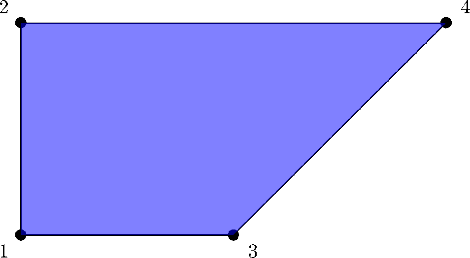
The sample space can be identified with the value of the sufficient statistics, hence with a finite subset of ℚ² ⊃ Ω, Ω = {(0, 0), (0, 1), (1, 0), (2, 1)}; see Figure 1. Given a finite subset of ℝ^d, it is a general algebraic fact that there exists a filtering set of monomial functions that is a vector basis of all real functions on the subset itself; see an exposition and the applications to statistics in [24] or [27]. In our case, the monomial basis is 1, T₁, T₂, T₁T₂, and we define the matrix of the saturated model to be:

$$\begin{array}{l}1T_1{T}_2{T}_1{T}_2\\ A=\begin{array}{l}1\\ 2\\ 3\\ 4\end{array}\left[\begin{array}{llll}1& 0& 0& 0\\ 1& 0& 1& 0\\ 1& 1& 0& 0\\ 1& 2& 1& 2\end{array}\right],A^{-1}=\frac{1}{2}\left[\begin{array}{llll}2& 0& 0& 0\\ -2& 0& 2& 0\\ -2& 2& 0& 0\\ 2& -1& -2& 1\end{array}\right].\end{array}$$

(14)

The matrix A one-to-one maps probabilities into expected values,

$$[\begin{array}{llll}1& {\eta }_1& {\eta }_2& {\eta }_{12}\end{array}]=\left[\begin{array}{llll}1& E\left[T_1\right]& E\left[T_2\right]& E\left[T_1{T}_2\right]\end{array}\right]=\left[\begin{array}{llll}{p}_1& p_2& p_3& p_4\end{array}\right]\left[\begin{array}{llll}1& 0& 0& 0\\ 1& 0& 1& 0\\ 1& 1& 0& 0\\ 1& 2& 1& 2\end{array}\right],$$

(15)

and vice versa,

$$\left[\begin{array}{llll}{p}_1& p_2& p_3& p_4\end{array}\right]=\left[\begin{array}{llll}1& {\eta }_1& {\eta }_2& {\eta }_{12}\end{array}\right]\left[\begin{array}{llll}1& 0& 0& 0\\ -1& 0& 1& 0\\ -1& 1& 0& 0\\ 1& -\frac{1}{2}& -1& \frac{1}{2}\end{array}\right].$$

(16)

On Model (13), the (positive) probabilities are constrained by the model:

$$\begin{array}{lll}\mathrm{\Omega }\hfill & p_{\mathit{\theta }}\hfill & \exp ({\theta }_1{T}_1+{\theta }_2{T}_2-\log (1+e^{{\theta }_2}+e^{{\theta }_1}+e^{2{\theta }_1+{\theta }_2}))\hfill \\ 1\hfill & p(1;\mathit{\theta })\hfill & \exp (-\log (1+e^{{\theta }_2}+e^{{\theta }_1}+e^{2{\theta }_1+{\theta }_2}))\hfill \\ 2\hfill & p(2;\mathit{\theta })\hfill & \exp ({\theta }_2-\log (1+e^{{\theta }_2}+e^{{\theta }_1}+e^{2{\theta }_1+{\theta }_2}))\hfill \\ 3\hfill & p(3;\mathit{\theta })\hfill & \exp ({\theta }_1-\log (1+e^{{\theta }_2}+e^{{\theta }_1}+e^{2{\theta }_1+{\theta }_2}))\hfill \\ 4\hfill & p(4;\mathit{\theta })\hfill & \exp (2{\theta }_1+{\theta }_2-\log (1+e^{{\theta }_2}+e^{{\theta }_1}+e^{2{\theta }_1+{\theta }_2}))\hfill \end{array}.$$

(17)

If we introduce the parameters ζ₁ = exp (θ₁), ζ₂ = exp (θ₂), the model is shown to be a (piece of an) algebraic variety, that is a set described by the rational parametric equations:

$$\begin{array}{lll}\mathrm{\Omega }\hfill & p_{\mathit{\zeta }}\hfill & {\zeta }^{T_1}{\zeta }^{T_2}/(1+{\zeta }_2+{\zeta }_1+{\zeta }_1^2{\zeta }_2)\hfill \\ 1\hfill & p(1;\mathit{\zeta })\hfill & 1/(1+{\zeta }_2+{\zeta }_1+{\zeta }_1^2{\zeta }_2)\hfill \\ 2\hfill & p(2;\mathit{\zeta })\hfill & {\zeta }_2/(1+{\zeta }_2+{\zeta }_1+{\zeta }_1^2{\zeta }_2)\hfill \\ 3\hfill & p(3;\mathit{\zeta })\hfill & {\zeta }_1/(1+{\zeta }_2+{\zeta }_1+{\zeta }_1^2{\zeta }_2)\hfill \\ 4\hfill & p(4;\mathit{\zeta })\hfill & {\zeta }_1^2{\zeta }_2/(1+{\zeta }_2+{\zeta }_1+{\zeta }_1^2{\zeta }_2)\hfill \end{array}.$$

(18)

The peculiar structure of the toric model is best seen by considering the unnormalized probabilities:

$$\begin{array}{lll}\mathrm{\Omega }\hfill & q_{\mathit{\zeta }}\hfill & {\zeta }^{T_1}{\zeta }^{T_2}\hfill \\ 1\hfill & q(1;\mathit{\zeta })\hfill & 1\hfill \\ 2\hfill & q(2;\mathit{\zeta })\hfill & {\zeta }_2\hfill \\ 3\hfill & q(3;\mathit{\zeta })\hfill & {\zeta }_1\hfill \\ 4\hfill & q(4;\mathit{\zeta })\hfill & {\zeta }_1^2{\zeta }_2\hfill \end{array},p(\mathit{x};\mathit{\zeta })=\frac{q(\mathit{x};\mathit{\zeta })}{1+{\zeta }_2+{\zeta }_1+{\zeta }_1^2{\zeta }_2}.$$

(19)

In algebraic terms, the homogeneous coordinates [q₁ : q₂ : q₃ : q₄] belong to the projective space P³. Precisely, the (real) projective space P³ is the set of all non-zero points of ℝ⁴ together with the equivalence relation $[q_1:q_2:q_3:q_4]=[{\overline{q}}_1:{\overline{q}}_2:{\overline{q}}_3:{\overline{q}}_4]$ if, and only if, $[q_1:q_2:q_3:q_4\left]=k\right[{\overline{q}}_1:{\overline{q}}_2:{\overline{q}}_3:{\overline{q}}_4]$, k ≠ 0. The domain of unnormalized signed probabilities as projective points is the open subset ${\mathbb{P}}_{*}^3$ of ℙ³ where q₁ + q₂ + q₃ + q₄ ≠ 0. On this set, we can compute the normalization:

$${\mathbb{P}}_{*}^3\ni [q_1:q_2:q_3:q_4]\mapsto [q_1,q_2,q_3,q_4]/(q_1+q_2+q_3+q_4){\in }^{\ast }ℰ,$$

where ^*ℇ is the affine space generated by the simplex Δ₃. Notice that this embedding produces a number of natural geometrical structures on ^*ℇ.

Because of the form of (13), a positive density p belongs to that family if, and only if, log p ∈ Span (1, T₁, T₂), which, in turn, is equivalent to log p ⊥ T₃. We can rewrite the orthogonality as:

$$\begin{array}{l}0={\displaystyle \sum _{\mathit{x}\in \mathrm{\Omega }}\log p(\mathit{x})T_3(\mathit{x})}={\displaystyle \sum _{\mathit{x}:T_3(\mathit{x})>0}\log p(\mathit{x})T_3^{+}(\mathit{x})}-{\displaystyle \sum _{\mathit{x}:T_3(\mathit{x})<0}\log p(\mathit{x})T_3^{-}(\mathit{x})}\\ =\log \left({\displaystyle \prod _{\mathit{x}:T_3(\mathit{x})>0}p(\mathit{x})T_3^{+}(\mathit{x})}\right)-\log \left({\displaystyle \prod _{\mathit{x}:T_3(\mathit{x})<0}p(\mathit{x})T_3^{-}(\mathit{x})}\right).\end{array}$$

Dropping the log function in the last expression, we observe that the positive probabilities described by either Equation (17) with θ₁, θ₂ ∈ ℝ or Equation (18) with ζ₁, ζ₂ ∈ ℝ_> are equivalently described by the equations:

$$p_1+p_2+p_3+p_4-1=0,$$

(20)

$$p_1^2{p}_4-p_2{p}_3^2=0.$$

(21)

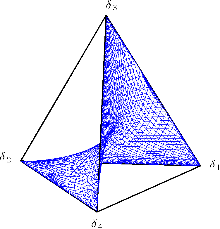
Equation (21) identifies a surface within the probability simplex Δ₃, which is represented in Figure 2 by the triangularization of a grid of points that satisfy the invariant.

By choosing a basis for the space orthogonal to Span (1, T₁, T₂)^⊥, we can embed the marginal polytope of Figure 1 into the associated full marginal polytope. By expressing probabilities as a function of the expectation parameters, Equation (21) identifies a relationship between η₁, η₂ and the expected values of the chosen basis for the orthogonal space. This corresponds to an equivalent invariant in the expectation parameters, which, in turn, identifies a surface in the full marginal polytope.

For instance, consider the full marginal polytope parametrized by η = (η₁, η₂, η₃), with ${\eta }_3=\mathrm{E}[T_3]$, which corresponds to the choice of T₃ as a basis for the space orthogonal to the span of the sufficient statistics of the model, together with the constant 1, as in Equation (12). We introduce the following matrix:

$$\begin{array}{l}1T_1{T}_2{T}_3\\ B=\begin{array}{l}1\\ 2\\ 3\\ 4\end{array}\left[\begin{array}{llll}1& 0& 0& -2\\ 1& 0& 1& 1\\ 1& 1& 0& 2\\ 1& 2& 1& -1\end{array}\right],\end{array}$$

(22)

and similarly to Equation (15), we use the B matrix to one-to-one map probabilities into expected values, that is:

$$\left[\begin{array}{l}1\\ {\eta }_1\\ {\eta }_2\\ {\eta }_3\end{array}\right]=\left[\begin{array}{llll}1& 1& 1& 1\\ 0& 0& 1& 2\\ 0& 1& 0& 1\\ -2& 1& 2& -1\end{array}\right]\left[\begin{array}{l}{p}_1\\ p_2\\ p_3\\ p_4\end{array}\right],$$

(23)

and:

$$\left[\begin{array}{l}{p}_1\\ p_2\\ p_3\\ p_4\end{array}\right]=\left[\begin{array}{llll}\frac{3}{5}& -\frac{1}{5}& -\frac{2}{5}& -\frac{1}{5}\\ \frac{1}{5}& -\frac{2}{5}& \frac{7}{10}& \frac{1}{10}\\ \frac{2}{5}& \frac{1}{5}& -\frac{3}{5}& \frac{1}{5}\\ -\frac{1}{5}& \frac{2}{5}& \frac{3}{10}& -\frac{1}{10}\end{array}\right]\left[\begin{array}{l}1\\ {\eta }_1\\ {\eta }_2\\ {\eta }_3\end{array}\right].$$

(24)

Then, by expressing probabilities as a function of the expectation parameters in Equation (21), we obtain the following invariant in η associated with the model:

$$(4{\eta }_1+3{\eta }_2-{\eta }_3-2){({\eta }_1+2{\eta }_2+{\eta }_3-3)}^2+(4{\eta }_1-7{\eta }_2-{\eta }_3-2){({\eta }_1-3{\eta }_2+{\eta }_3+2)}^2=0.$$

(25)

From the linear relationship between probabilities and expectation probabilities, we know that on the interior of the full marginal polytope, there exists a unique η₃ which can be computed as a function of the other expectation parameters. Solving Equation (25) for η₃ allows one to express explicitly the value of η₃ given (η₁, η₂) and represent the surface associated with the invariant in the full marginal polytope. However, the cubic polynomial in Equation (25) in general admits three roots. The unique value of η₃ can be obtained from the roots of the cubic polynomial, by imposing that η₃ must be real and belong to the full marginal polytope given by Conv {(T₁(x), T₂(x), T₃(x))|x ∈ Ω}.

We remind that the determinant Δ associated with the cubic function in Equation (25) in the η₃ variable:

$$a{\eta }_3^3+b{\eta }_3^2+c{\eta }_3+d=0,$$

(26)

with:

$$a=1$$

(27)

$$b=-2{\eta }_1+{\eta }_2+1$$

(28)

$$\begin{array}{l}c=-(4{\eta }_1+3{\eta }_2-2)({\eta }_1+2{\eta }_2-3)+\frac{1}{2}{({\eta }_1+2{\eta }_2-3)}^2-(4{\eta }_1+7{\eta }_2-2)({\eta }_1-3{\eta }_2+2)+\\ +\frac{1}{2}{({\eta }_1-3{\eta }_2+2)}^2\end{array}$$

(29)

$$d=-\frac{1}{2}(4{\eta }_1+3{\eta }_2-2){({\eta }_1+2{\eta }_2-3)}^2-\frac{1}{2}(4{\eta }_1-7{\eta }_2-2){({\eta }_1-3{\eta }_2+2)}^2$$

(30)

is given by:

$$\mathrm{\Delta }=18abcd-4b^{3}d+b^2{c}^2-4a{c}^3-27a^2{d}^2.$$

(31)

For Δ = 0, the polynomial has a real root with multiplicity equal to three; for Δ < 0, we have one real root and two complex conjugates roots, while for Δ > 0, there exist three real roots. The three roots of the polynomial as a function of the coefficients are given by:

$${\eta }_{3,k}=-\frac{1}{3}\left(b+u_{k}C+\frac{{\mathrm{\Delta }}_0}{u_{k}C}\right),$$

(32)

for k ∈ {1, 2, 3}, with:

$$u_1=1,$$

(33)

$$u_2=\frac{-1+i\sqrt{3}}{2},$$

(34)

$$u_3=\frac{-1-i\sqrt{3}}{2},$$

(35)

and:

$$C=\sqrt[3]{\frac{{\mathrm{\Delta }}_1+\sqrt{\left({\mathrm{\Delta }}_1^2-4{\mathrm{\Delta }}_0^3\right)}}{2}},$$

(36)

$${\mathrm{\Delta }}_0=b^2-3ac,$$

(37)

$${\mathrm{\Delta }}_1=2b^3+9abc+27a^{2}d.$$

(38)

For the cubic polynomial in η₃ of Equation (25), Δ < 0 for η₂ − 1 ≠ 0 and for:

$$4{\eta }_1^4-8{\eta }_1^3{\eta }_2+24{\eta }_1^2{\eta }_2^2-20{\eta }_1{\eta }_2^3-2{\eta }_2^4-8{\eta }_1^3-12{\eta }_1^2{\eta }_2+4{\eta }_2^3+8{\eta }_1^2+16{\eta }_1{\eta }_2-{\eta }_2^2-4{\eta }_1-2{\eta }_2+1>0.$$

(39)

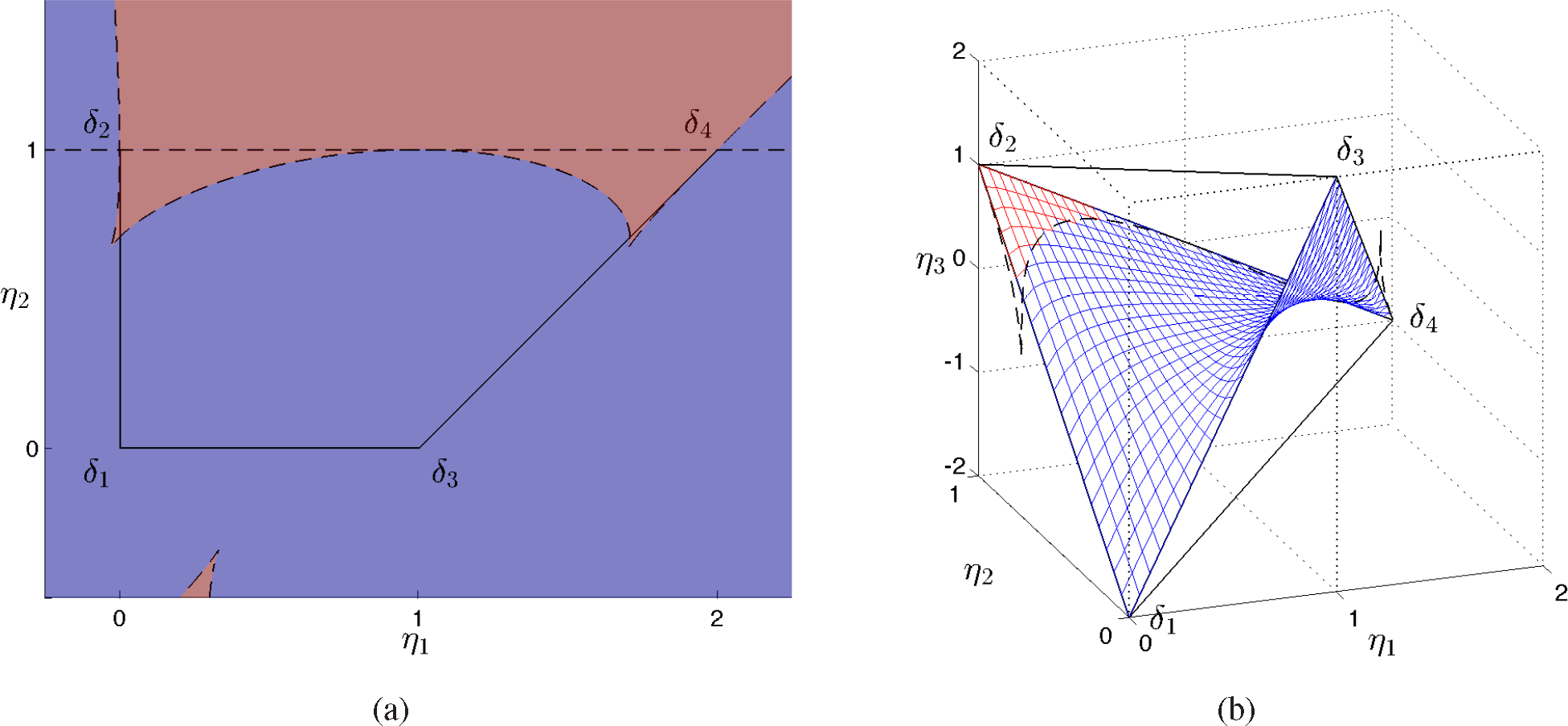
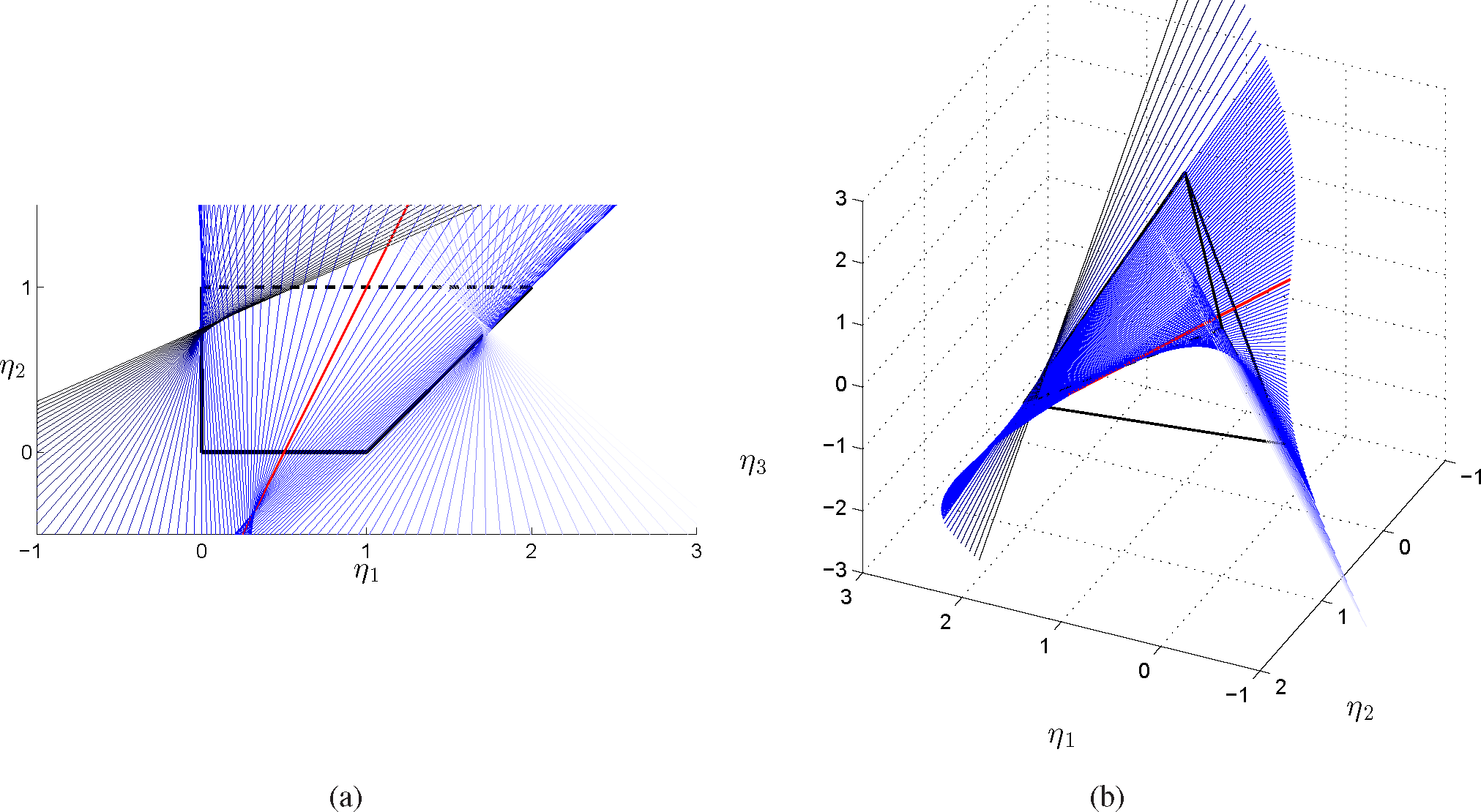
In Figure 3(a), we represent in blue the region of the space (η₁, η₂) where Δ < 0, in red where Δ > 0, and the points where Δ = 0 with a dashed line. For Δ < 0, the only real root is η_3,1, which identifies the blue surface in the full marginal polytope in Figure 3(b). For Δ > 0, it is easy to verify that only η_3,2 belongs to the interior of the full marginal polytope parametrized by (η₁, η₂, η₃), since it satisfies the inequalities given by the facets of the marginal polytope, and is represented in Figure 3(b) by the red surface. Finally, the three real roots coincide for Δ = 0, that is, for η₂ = 1, and where:

$$4{\eta }_1^4-8{\eta }_1^3{\eta }_2+24{\eta }_1^2{\eta }_2^2-20{\eta }_1{\eta }_2^3-2{\eta }_2^4-8{\eta }_1^3-12{\eta }_1^2{\eta }_2+4{\eta }_2^3+8{\eta }_1^2+16{\eta }_1{\eta }_2-{\eta }_2^2-4{\eta }_1-2{\eta }_2+1=0.$$

(40)

In the polynomial ring ℚ [p₁, p₂, p₃, p₄], the model ideal:

$$I=\langle p_1+p_2+p_3+p_4-1,p_1^2{p}_4-p_2{p}_3^2\rangle$$

(41)

consists of all the polynomials of the form:

$$A=(p_1+p_2+p_3+p_4-1)+B(p_1^2{p}_4-p_2{p}_3^2),\forall A,B\in \mathbb{Q}[p_1,p_2,p_3,p_4].$$

The algebraic variety of $\mathrm{I}$ uniquely extends the exponential family outside the positive octant. In the language of commutative algebra, it is the real Zariski closure of the exponential family model, cf. [29]. It is a notable example of toric variety. The general theory is in the monograph [30], and the applications to statistical models were first discussed in [31,32].

Let us discuss in some detail the parameterization of the toric variety as the submanifold of ℝ⁴ defined by Equations (20) and (21). The Jacobian matrix is:

$$J=\left[\begin{array}{llll}1\hfill & 1\hfill & 1\hfill & 1\hfill \\ 2p_1{p}_4\hfill & -p_3^2\hfill & -2p_2{p}_3\hfill & p_1^2\hfill \end{array}\right].$$

It has rank one, that is, there is a singularity, if, and only if,

$$2p_1{p}_4=-p_3^2=-2p_2{p}_3=p_1^2.$$

This is equivalent to $p_1^2=p_3^2=0$, which is a subspace of dimension two, whose intersection with Equation (20), is a line $\mathrm{C}$ in the affine space ^*ℇ = {p ∈ ℝ⁴|p₁ + p₂ + p₃ + p₄ = 1}. This (double) critical line intersects the simplex along the edge δ₂ ↔ δ₄. Outside $\mathrm{C}$, that is in the open complement set, the equations of the toric variety are locally solvable in two among the p_i’s under the condition that the corresponding minor is not zero. To have a picture of what this critical set looks like, let us intersect our surface with the plane p₃ = 0. On the affine space p₁ + p₂ + p₄ = 1 we have $p_1^2{p}_4=0$, that is the union of the double line $p_1^2=0$ with the line p₄ = 0.

In the following, we derive a parameterization based on an algebraic argument, the Bézout theorem. In fact, it is remarkable that the cubic surface defined by Equations (20) and (21) is a well known example of ruled surface, see Exercise 5.8.15 in [33]. In fact, the singular line is a double line, so that the intersection of the cubic surface with any plane through the singular line is of degree 1 = 3 − 2, by the Bézout theorem, and thus, it is a line.

The line $\mathrm{C}$ is said to be double because the polynomial $p_1^2{p}_4-p_2{p}_3^2$ belongs to the ideal generated by $p_1^2$ and $p_3^2$. Let us consider the sheaf of planes through the singular line defined for each [α : β] ∈ P¹ by the equations:

$$\mathcal{P}[\alpha :\beta ]=\{p_1+p_2+p_3+p_4-1=0,\alpha p_1+\beta p_3=0\}.$$

Let us intersect each plane $\mathcal{P}[\alpha :\beta ]$ of the sheaf with the model variety $\mathcal{M}$ by solving the system of equations:

$$\{\begin{array}{ll}{p}_1+p_2+p_3+p_4& =1\\ p_1^2{p}_4-p_2{p}_3^2& =0\\ \alpha p_1+\beta p_3& =0\end{array}.$$

(42)

On the critical line $\mathrm{C}$, a generic point is parameterized as p(τ, 0) = (0, τ, 0, 1 − τ), which satisfies Equation (42) for τ ∈ ℝ. If 0 ≤ τ ≤ 1, then p(τ, 0) belongs to the edge δ₂ ↔ δ₄.

As the critical line is double and the intersection of the model variety with the plane of the sheaf is a cubic curve, we expect the remaining part to be of degree 3 − 2 = 1, that is to be a line. Assume first α, β ≠ 0. Outside the critical line, as p₁, p₃ are not both zero and αp₁ + βp₃ = 0, then αp₁ = − βp₃ ≠ 0. It follows (αp₁)² = (βp₃)²≠ 0; hence:

$$p_1^2{p}_4-p_2{p}_3^2=0\Rightarrow {\beta }^2{(\alpha p_1)}^2{p}_4-{\alpha }^2{p}_2{(\beta p_3)}^2=0\Rightarrow {\beta }^2{p}_4-{\alpha }^2{p}_2=0.$$

We have found that for α, β ≠ 0, the intersection between the plane $\mathcal{P}[\alpha :\beta ]$ and the model variety $\mathcal{M}$ is the union of the critical line $\mathrm{C}$ and the line of equations:

$$\{\begin{array}{ll}{p}_1+p_2+p_3+p_4& =1\\ \alpha p_1+\beta p_3& =0\\ -{\alpha }^2{p}_2+{\beta }^2{p}_4& =0\end{array}.$$

(43)

This line intersects the critical line where:

$$p_1=p_3=0,p_2+p_4=1,-{\alpha }^2{p}_2+{\beta }^2{p}_4=0,$$

that is in the point:

$$\mathit{p}([\alpha :\beta ],0))=\left(0,\frac{{\beta }^2}{{\alpha }^2+{\beta }^2},0,\frac{{\alpha }^2}{{\alpha }^2+{\beta }^2}\right).$$

In parametric form, the line in Equations (43) is:

$$\mathit{p}([\alpha :\beta ],t)=\mathit{p}([\alpha :\beta ],0)+\mathit{u}t,$$

with $\mathit{u}=\left(\beta ,\frac{{\beta }^2(\alpha -\beta )}{{\alpha }^2+{\beta }^2},-\alpha ,\frac{{\alpha }^2(\alpha -\beta )}{{\alpha }^2+{\beta }^2}\right),$

$$\begin{array}{l}{p}_1([\alpha :\beta ],t)=\beta t\\ p_2([\alpha :\beta ],t)=\frac{{\beta }^2}{{\alpha }^2+{\beta }^2}+\frac{{\beta }^2(\alpha -\beta )}{{\alpha }^2+{\beta }^2}t\\ p_3([\alpha :\beta ],t)=-\alpha t\\ p_4([\alpha :\beta ],t)=\frac{{\alpha }^2}{{\alpha }^2+{\beta }^2}+\frac{{\alpha }^2(\alpha -\beta )}{{\alpha }^2+{\beta }^2}t.\end{array}$$

(44)

The same equations hold in the previously excluded case αβ = 0.

Positive values of components 1 and 3 of the probability are obtained in Equation (44) for αβ < 0 and βt > 0, say α < 0, β > 0, t > 0. In this case, we have for component 2:

$$\frac{{\beta }^2}{{\alpha }^2+{\beta }^2}+\frac{{\beta }^2(\alpha -\beta )}{{\alpha }^2+{\beta }^2}t=\frac{{\beta }^2}{{\alpha }^2+{\beta }^2}(1-(\beta -\alpha )t),$$

which is positive if t < (β − α)⁻¹. The same condition applies to component 4. As $[\alpha :\beta ]=\left[\frac{\alpha }{\beta -\alpha }:\frac{\beta }{\beta -\alpha }\right]$, we can always assume β > 0 and β − α = 1 that is, α = β − 1; hence β < 1. The parameterization of the positive probabilities in the model becomes:

$$\begin{array}{l}{p}_1(\alpha ,t)=(\alpha +1)t\\ p_2(\alpha ,t)=\frac{{\alpha }^2-({\alpha }^2+2\alpha +1)t+2\alpha +1}{2{\alpha }^2+2\alpha +1}\\ p_3(\alpha ,t)=-\alpha t\\ p_4(\alpha ,t)=-\frac{{\alpha }^{2}t-{\alpha }^2}{2{\alpha }^2+2\alpha +1}\end{array},0<t<1,-1<\alpha <0.$$

(45)

For example, with $\alpha =-\frac{1}{2}$, we have:

$$\begin{array}{l}{p}_1(\alpha ,t)=\frac{1}{2}t\\ p_2(\alpha ,t)=\frac{1}{2}(1-t)\\ p_3(\alpha ,t)=\frac{1}{2}t\\ p_4(\alpha ,t)=\frac{1}{2}(1-t)\end{array},0<t<1.$$

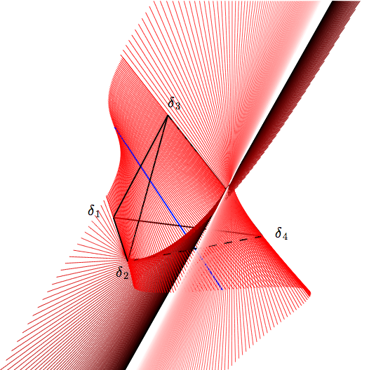
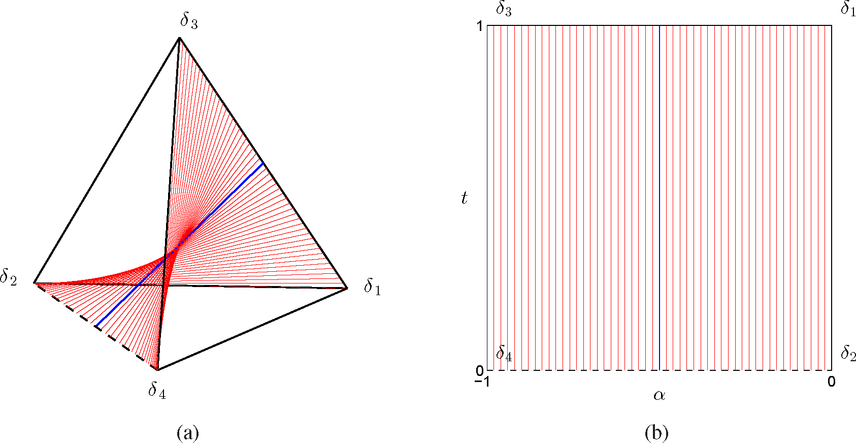
In Figure 4(a), we represented the surface associated with the invariant of Equation (21) as a ruled surface in the probability simplex, according to Equations (45), where the blue line corresponds to the case $\alpha =-\frac{1}{2}$. The ruled surface corresponds to the surface in Figure 2 that was approximated by the triangularization of a grid of points satisfying the invariant. In Figure 4(b), we represent the same lines of Figure 4(a) in the chart (α, t).

From Equation (45), we can express the expectation parameters η as a function of (α, t), i.e.,

$${\eta }_1=\frac{2{\alpha }^2-(2{\alpha }^3+4{\alpha }^2+\alpha )t}{2{\alpha }^2+2\alpha +1},$$

(46)

$${\eta }_2=-t+1,$$

(47)

$${\eta }_3=-\frac{(8{\alpha }^3+12{\alpha }^2+10\alpha +3)t-2\alpha -1}{2{\alpha }^2+2\alpha +1}.$$

(48)

Notice that the dependence on (α, t) is rational. In Figure 5(a), the ruled surface has been represented in the full marginal polytope, while in Figure 5(a), the lines have been projected over the marginal polytope.

Let us invert Equation (45) to obtain the corresponding chart p ↦ (β, t). From p₁ and p₃, we obtain β = p₁/(p₁ + p₃). As p₂ + p₄ = 1 − t, we have the chart:

$$\begin{array}{l}\beta =\frac{p_1}{p_1+p_3},\\ t=1-p_2-p_4=p_1+p_3.\end{array}$$

It is remarkable that the model depends on the probability restricted to {1, 3}; similarly, the expectation parameters depend on p₁ and p₃ only.

From the theory of exponential families, we know that the gradient mapping:

$$({\theta }_1,{\theta }_2)\mapsto \nabla \psi ({\theta }_1,{\theta }_2)=\left[\frac{2e^{(2{\theta }_1+{\theta }_2)}+e^{{\theta }_1}}{e^{(2{\theta }_1+{\theta }_2)}+e^{{\theta }_1}+e^{{\theta }_2}+1}\frac{e^{(2{\theta }_1+{\theta }_2)}+e^{{\theta }_2}}{e^{(2{\theta }_1+{\theta }_2)}+e^{{\theta }_1}+e^{{\theta }_2}+1}\right]$$

is one-to-one from ℝ² onto the interior of the marginal polytope M; see Figure 3(b). The equations:

$$\begin{array}{l}{\eta }_1=\frac{{\zeta }_1+2{\zeta }_1^2{\zeta }_2}{1+{\zeta }_2+{\zeta }_1+{\zeta }_1^2{\zeta }_2},\\ {\eta }_2=\frac{{\zeta }_2+{\zeta }_1^2{\zeta }_2}{1+{\zeta }_2+{\zeta }_1+{\zeta }_1^2{\zeta }_2},\end{array}$$

are uniquely solvable for (η₁, η₂) ∈ M°. We study the local solvability in ζ₁, ζ₂ of:

$$\begin{array}{l}(1+{\zeta }_2+{\zeta }_1+{\zeta }_1^2{\zeta }_2){\eta }_1={\zeta }_1+2{\zeta }_1^2{\zeta }_2,\\ (1+{\zeta }_2+{\zeta }_1+{\zeta }_1^2{\zeta }_2){\eta }_2={\zeta }_2+{\zeta }_1^2{\zeta }_2,\end{array}$$

that is,

$$\begin{array}{l}0={\eta }_1+({\eta }_1-1){\zeta }_1+{\eta }_1{\zeta }_2+({\eta }_1-2){\zeta }_1^2{\zeta }_2,\\ 0={\eta }_2+{\eta }_2{\zeta }_1+({\eta }_2-1){\zeta }_2+({\eta }_2-1){\zeta }_1^2{\zeta }_2.\end{array}$$

The Jacobian is:

$$\left[\begin{array}{ll}({\eta }_1-1)+2({\eta }_1-2){\zeta }_1{\zeta }_2& {\eta }_1+({\eta }_1-2){\zeta }_1^2\\ {\eta }_2+2({\eta }_2-1){\zeta }_1{\zeta }_2& ({\eta }_2-1)+({\eta }_2-1){\zeta }_1^2\end{array}\right].$$

If we introduce the extra variable η₁₂, from Equations (15) and (18) we have the system:

$$\begin{array}{l}(1+{\zeta }_2+{\zeta }_1+{\zeta }_1^2{\zeta }_2){\eta }_1={\zeta }_1+2{\zeta }_1^2{\zeta }_2,\\ (1+{\zeta }_2+{\zeta }_1+{\zeta }_1^2{\zeta }_2){\eta }_2={\zeta }_2+{\zeta }_1^2{\zeta }_2,\\ (1+{\zeta }_2+{\zeta }_1+{\zeta }_1^2{\zeta }_2){\eta }_{12}=2{\zeta }_1^2{\zeta }_2,\end{array}$$

Instead, if we use the variable η₃, from Equations (16) and (41), it is possible to derive the equation of the model variety in the η₁, η₂, η₃ parameters. From Equation (18), we have:

$$\begin{array}{l}{\eta }_1={\mathrm{E}}_{\mathit{\zeta }}[T_1]=\frac{{\zeta }_1+2{\zeta }_1^2{\zeta }_2}{1+{\zeta }_2+{\zeta }_1+{\zeta }_1^2{\zeta }_2},\\ {\eta }_2={\mathrm{E}}_{\mathit{\zeta }}[T_2]=\frac{{\zeta }_2+{\zeta }_1^2{\zeta }_2}{1+{\zeta }_2+{\zeta }_1+{\zeta }_1^2{\zeta }_2},\\ {\eta }_3={\mathrm{E}}_{\mathit{\zeta }}[T_3]=\frac{-2+{\zeta }_2+2{\zeta }_1-{\zeta }_1^2{\zeta }_2}{1+{\zeta }_2+{\zeta }_1+{\zeta }_1^2{\zeta }_2}.\end{array}$$

Let us solve for the ζ, that is:

There is another way to derive the model constraint in the η. In the example, the sample space has four points; the monomials 1, T₁, T₂, T₁T₂ are a vector basis of the linear space of the columns of the matrix A, in particular T₃ is a linear combination:

$$\begin{array}{llllll}\mathrm{\Omega }\hfill & 1\hfill & T_1\hfill & T_2\hfill & T_1{T}_2\hfill & T_3\hfill \\ 1\hfill & 1\hfill & 0\hfill & 0\hfill & 0\hfill & -2\hfill \\ 2\hfill & 1\hfill & 0\hfill & 1\hfill & 0\hfill & 1\hfill \\ 3\hfill & 1\hfill & 1\hfill & 0\hfill & 0\hfill & 2\hfill \\ 4\hfill & 1\hfill & 2\hfill & 1\hfill & 2\hfill & -1\hfill \\ \hfill & -2\hfill & 4\hfill & 3\hfill & -5\hfill & =\hfill \end{array}$$

It follows that:

$$\begin{array}{l}{\eta }_3={\mathrm{E}}_{\mathit{\theta }}[T_3]={\mathrm{E}}_{\mathit{\theta }}[-2+4T_1+3T_2-5T_1{T}_2]\\ =-2+4{\mathrm{E}}_{\mathit{\theta }}[T_1]+3{\mathrm{E}}_{\mathit{\theta }}[T_2]+3{\text{Cov}}_{\mathit{\theta }}(T_1,T_2)+3{\mathrm{E}}_{\mathit{\theta }}[T_1]{\mathrm{E}}_{\mathit{\theta }}[T_2]\\ =-2+4{\partial }_1\psi (\mathit{\theta })+3{\partial }_2\psi (\mathit{\theta })-5{\partial }_1{\partial }_2\psi (\mathit{\theta })-5{\partial }_1\psi (\mathit{\theta }){\partial }_2\psi (\mathit{\theta })\\ =-2+4{\eta }_1+3{\eta }_2-5{\partial }_1{\partial }_2\psi (\mathit{\theta })-5{\eta }_1{\eta }_2.\end{array}$$

3.1. Border

Let us consider the points in the model variety that are probabilities, that is,

$$p_1+p_2+p_3+p_4=1,p_1^2{p}_4=p_2{p}_3^2,p_1,p_2,p_3,p_4\ge 0.$$

(49)

From the equation above, we see that single zeros are not allowed, that is to say there are no intersections between the model in Equation (49) and the open facets of the probability simplex. We now consider the full marginal polytope obtained by adding the sufficient statistics T₁T₂, and parametrized by (η₁, η₂, η₁₂). By Equation (16), the marginal polytope is represented by the inequalities:

$$\begin{array}{l}{p}_1=1-{\eta }_1-{\eta }_2+{\eta }_{12}\ge 0,\\ p_2={\eta }_2-\frac{1}{2}{\eta }_{12}\ge 0,\\ p_3={\eta }_1-{\eta }_{12}\ge 0,\\ p_4=\frac{1}{2}{\eta }_3\ge 0,\end{array}$$

which is a convex set with vertexes (0, 0, 0), (0, 1, 0), (1, 0, 0), (2, 1, 2), which corresponds to the full marginal polytope associated to the sufficient statistics {T₁, T₂, T₁T₂}. As the critical set is the edge δ₂ ↔ δ₄ in the p space, it is the edge (0, 1, 0) ↔ (2, 1, 2) in the η space.

We have the following possible models on the border of the probability simplex and on the border of the full marginal polytope, where the values for η₁ and η₂ are obtained from Equation (15).

$$\begin{array}{llllll}{p}_1\hfill & p_2\hfill & p_3\hfill & p_4\hfill & {\eta }_1\hfill & {\eta }_2\hfill \\ 0\hfill & 0\hfill & +\hfill & +\hfill & p_3+2p_4\hfill & p_4\hfill \\ 0\hfill & +\hfill & 0\hfill & +\hfill & 2p_4\hfill & p_2+p_4\hfill \\ +\hfill & 0\hfill & +\hfill & 0\hfill & p_3\hfill & 0\hfill \\ +\hfill & +\hfill & 0\hfill & 0\hfill & 0\hfill & p_2\hfill \end{array}\begin{array}{llllll}{p}_1\hfill & p_2\hfill & p_3\hfill & p_4\hfill & {\eta }_1\hfill & {\eta }_2\hfill \\ +\hfill & 0\hfill & 0\hfill & 0\hfill & 0\hfill & 0\hfill \\ 0\hfill & +\hfill & 0\hfill & 0\hfill & 0\hfill & 1\hfill \\ 0\hfill & 0\hfill & +\hfill & 0\hfill & 1\hfill & 0\hfill \\ 0\hfill & 0\hfill & 0\hfill & +\hfill & 2\hfill & 1\hfill \end{array}$$

That is, the domains that can be support of probabilities in the algebraic model are the faces of the marginal polytope. This is general; see [20,34].

3.2. Fisher Information

Let us consider the covariance matrix of the sufficient statistics. Let us denote by A_|12 the block of the two central columns in A in Equation (14) and by p the row vector of probabilities. Then, the variance matrix is:

$$A_{|12}^T\mathrm{diag}(\mathit{p})A_{|12}-{(\mathit{p}{A}_{|12})}^T\mathit{p}{A}_{|12}=A_{|12}^T\mathrm{diag}(\mathit{p})A_{|12}-A_{|12}^T{\mathit{p}}^T\mathit{p}{A}_{|12}=A_{|12}^T(\mathrm{diag}(\mathit{p})-{\mathit{p}}^T\mathit{p})A_{|12}.$$

On each of the cases of probabilities supported by a single point, the matrix p − p^T p is zero; hence, the covariance matrix is zero. In each of the cases where the probability is supported by a facet, say {1, 2}, the matrix p − p^T p reduces to the corresponding block, and the covariance matrix is:

$$\begin{array}{l}\left[\begin{array}{llll}0\hfill & 0\hfill & 1\hfill & 1\hfill \\ 0\hfill & 1\hfill & 0\hfill & 1\hfill \end{array}\right]\left[\begin{array}{llll}{p}_1-p_1^2& -p_1{p}_2& 0& 0\\ -p_1{p}_2& p_2-p_2^2& 0& 0\\ 0& 0& 0& 0\\ 0& 0& 0& 0\end{array}\right]\left[\begin{array}{ll}0\hfill & 0\hfill \\ 0\hfill & 1\hfill \\ 1\hfill & 0\hfill \\ 2\hfill & 1\hfill \end{array}\right]\\ =\left[\begin{array}{ll}0& 0\\ 0& 1\end{array}\right]\left[\begin{array}{ll}{p}_1-p_1^2& -p_1{p}_2\\ -p_1{p}_2& p_2-p_2^2\end{array}\right]\left[\begin{array}{ll}0& 0\\ 0& 1\end{array}\right]\\ =\left[\begin{array}{ll}0& 0\\ 0& p_2-p_2^2\end{array}\right].\end{array}$$

The space generated by the covariance matrix is ℚ (0, 1), that is the affine space that contains the facets itself. Analogous results hold for each facet, and this result is general.

We note that the determinant of the covariance matrix is a polynomial of degree six in the indeterminates p₁, p₂, p₃. This polynomial is zero on each facet.

The η parameters can be given as a function of either θ or ζ. We have:

$$\begin{array}{ll}\mathit{\eta }\hfill & A^T[p\mathit{\zeta }]\hfill \\ {\eta }_1\hfill & ({\zeta }_1+2{\zeta }_1^2{\zeta }_2)/(1+{\zeta }_2+{\zeta }_1+{\zeta }_1^2{\zeta }_2)\hfill \\ {\eta }_2\hfill & ({\zeta }_2+{\zeta }_1^2{\zeta }_2)/(1+{\zeta }_2+{\zeta }_1+{\zeta }_1^2{\zeta }_2)\hfill \\ {\eta }_3\hfill & (-2+{\zeta }_2+2{\zeta }_1-{\zeta }_1^2{\zeta }_2)/(1+{\zeta }_2+{\zeta }_1+{\zeta }_1^2{\zeta }_2)\hfill \end{array}$$

(50)

We know from the theory of exponential families that the mapping:

$$]0,\infty [\times ]0,\infty [∍({\zeta }_1,{\zeta }_2)\mapsto ({\eta }_1,{\eta }_2)\in \text{Conv}\{(T_1(x),T_2(x))|x\in \mathrm{\Omega }\}°$$

is one-to-one. We look for an algebraic inversion of the equations:

$$\begin{array}{l}(1+{\zeta }_2+{\zeta }_1+{\zeta }_1^2{\zeta }_2){\eta }_1={\zeta }_1+2{\zeta }_1^2{\zeta }_2,\\ (1+{\zeta }_2+{\zeta }_1+{\zeta }_1^2{\zeta }_2){\eta }_2={\zeta }_2+{\zeta }_1^2{\zeta }_2.\end{array}$$

If we rewrite Equations (50) as polynomials in ζ₁, ζ₂, we obtain:

$${\eta }_1+({\eta }_1-1){\zeta }_1+{\eta }_1{\zeta }_2+({\eta }_1-2){\zeta }_1^2{\zeta }_2=0,$$

(51)

$${\eta }_2+{\eta }_2{\zeta }_1+({\eta }_2-1){\zeta }_2+({\eta }_2-1){\zeta }_1^2{\zeta }_2=0,$$

(52)

$$-{\eta }_3+({\eta }_3-2){\zeta }_1+({\eta }_3-1){\zeta }_2+({\eta }_3+1){\zeta }_1^2{\zeta }_2=0.$$

(53)

Gauss elimination produces a linear system in ζ₁, ζ₂ with coefficients that are polynomials in η₁, η₂, η₃ to be considered with the implicit equation derived from $p_1^2{p}_4-p_2{p}_3^2=0$. The system is:

$$\begin{array}{c}-2{\eta }_2{\eta }_3-2{\eta }_1+2{\eta }_2=(-2{\eta }_2{\eta }_3-2{\eta }_1+2){\zeta }_1+(-2{\eta }_2{\eta }_3+2{\eta }_2+2{\eta }_3-2){\zeta }_2,\\ {\eta }_2={\eta }_2\zeta 1+({\eta }_2-1){\zeta }_2.\end{array}$$

3.3. Extension of the Model

In this subsection, we study an extension to signed probabilities of the exponential family in Equations (12) and (13) based on the representation of the statistical model as a ruled surface in the probability simplex. Our motivation for such an analysis is the study of the stability of the critical points of a gradient field in the η parameters, in particular when the critical points belong to the boundary of the model. Indeed, by extending the gradient field outside the marginal polytope, we can identify open neighborhoods for critical points on the boundary of the polytope, which allow one to study the convergence of the differential equations associated with the gradient flows, for instance by means of Lyapunov stability.

In the following, we describe more in detail how the extension can be obtained. Let a be a point along the edge δ₂ ↔ δ₄ of the full marginal polytope parametrized by (η₁, η₂, η₃) and b the coordinates of the corresponding point over δ₁ ↔ δ₃ obtained by intersecting the line of the ruled surface through a with the edge δ₁ ↔ δ₃. The values of the η₂ coordinate for a and b are one and zero, respectively. The other coordinates of b depend on those of a though α. First, we obtain the values of the η₃ coordinates as a function of the η₁ coordinate. For a, we find the equation of the line to which δ₂ ↔ δ₄ belongs, given by:

$$\left(\begin{array}{l}{\eta }_1\\ {\eta }_2\\ {\eta }_3\end{array}\right)=\left(\begin{array}{l}0\\ 1\\ 1\end{array}\right)+u\left(\begin{array}{l}2\\ 0\\ -2\end{array}\right)=\left(\begin{array}{l}2u\\ 1\\ 1-2u\end{array}\right),$$

(54)

from which we obtain η₃ = 1 − η₁. Similarly, for the η₃ coordinate of b, we consider the line through δ₁ ↔ δ₃, that is:

$$\left(\begin{array}{l}{\eta }_1\\ {\eta }_2\\ {\eta }_3\end{array}\right)=\left(\begin{array}{l}0\\ 0\\ -2\end{array}\right)+u\left(\begin{array}{l}1\\ 0\\ 4\end{array}\right)=\left(\begin{array}{l}u\\ 0\\ 4u-2\end{array}\right),$$

(55)

which gives us η₃ = 4η₁ − 2. Finally, for the η₁ coordinate, we use Equations (44). In a, since t = 0 and p₁ = p₃ = 0, then $p_2=\frac{{\beta }^2}{{\alpha }^2+{\beta }^2}$ and $p_4=\frac{{\alpha }^2}{{\alpha }^2+{\beta }^2}$. From Equation (24), it follows that:

$${\eta }_1=\frac{2{\alpha }^2}{2{\alpha }^2+2\alpha +1}.$$

(56)

Similarly, for b, we have p₂ = p₄ = 0 and t = 1, so that p₁ = α + 1 and p₃ = −α. From Equation (24), it follows that:

$${\eta }_1=-\alpha .$$

(57)

As a result, the coordinates of a and b both depend on α as follows,

$$\mathit{a}=\left(\frac{2{\alpha }^2}{2{\alpha }^2+2\alpha +1},1,\frac{2\alpha +1}{2{\alpha }^2+2\alpha +1}\right)$$

(58)

$$\mathit{b}=(-\alpha ,0,-4\alpha -2)$$

(59)

The ruled surface in the full marginal polytope is given by the lines through a and b described by the following implicit representation, for −1 < α < 1 and 0 < t < 1,

$$\left[\begin{array}{l}{\eta }_1\\ {\eta }_2\\ {\eta }_3\end{array}\right]=\left[\begin{array}{l}-\alpha \\ 0\\ -4\alpha -2\end{array}\right]+t\left[\begin{array}{l}\frac{2{\alpha }^3+4{\alpha }^2+\alpha }{2{\alpha }^2+2\alpha +1}\\ 1\\ \frac{8{\alpha }^3+12{\alpha }^2+10\alpha +3}{2{\alpha }^2+2\alpha +1}\end{array}\right].$$

(60)

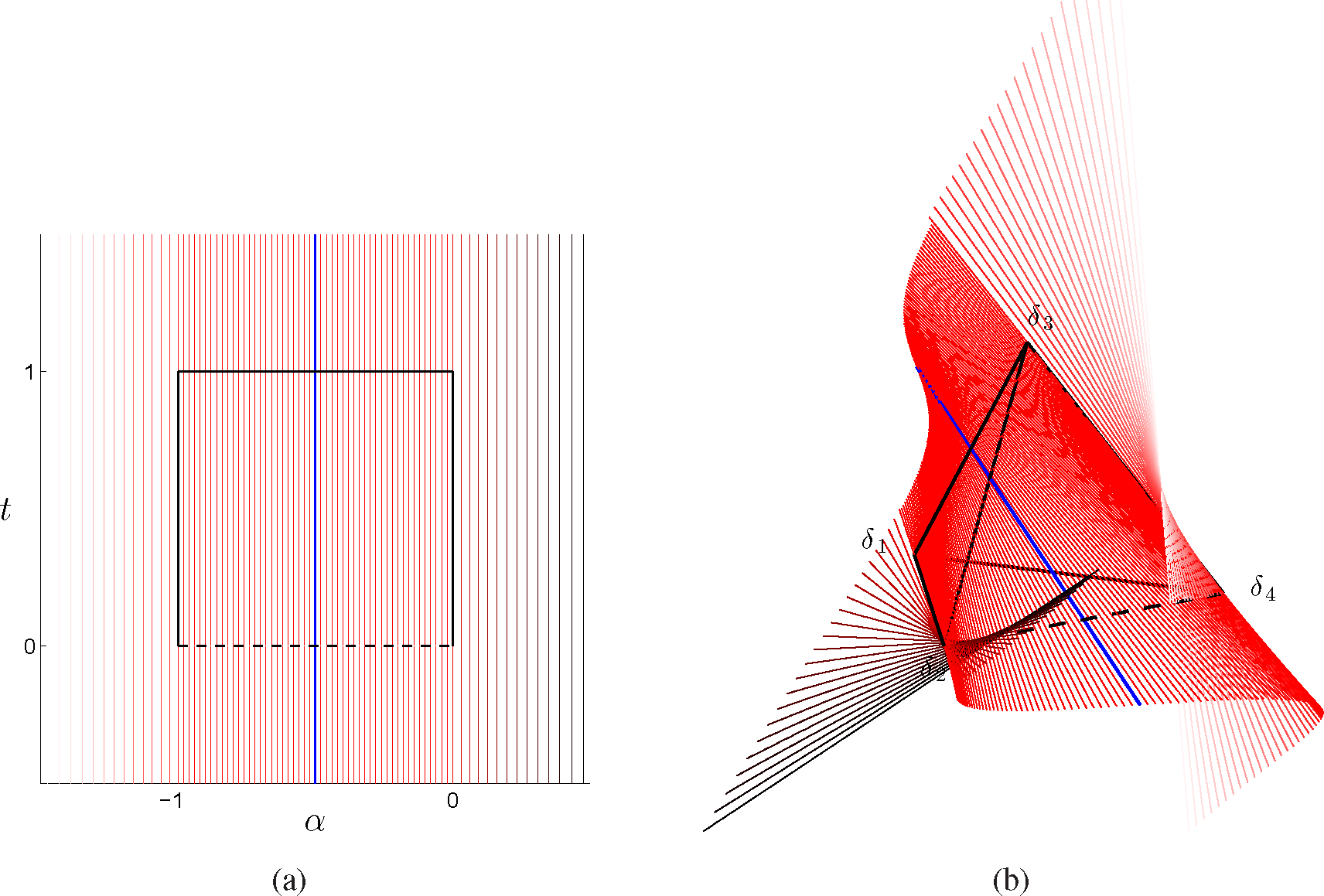
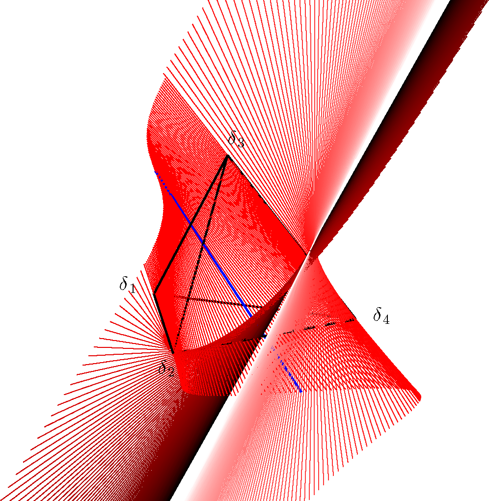
The ruled surface can be extended outside the marginal polytope by taking values of α, t ∈ ℝ and considering the set of lines through a and b for different values of α. For α → ±∞, the η₁ coordinate of b tends to ∓∞, while the η₁ of a tends to one. For α → ±∞, the ruled surface admits the same limit given by the line parallel to δ₁ ↔ δ₃ passing through (1, 1, 0). The surface intersects the interior of the marginal polytope for t ∈ (0, 1) and α ∈ (−1, 0). Moreover, the surface intersects the critical line twice, for t = 0, α ∈ [−1, 0] and for t = 0, α ∉ [−1, 0].

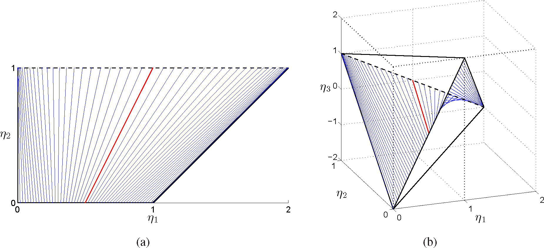
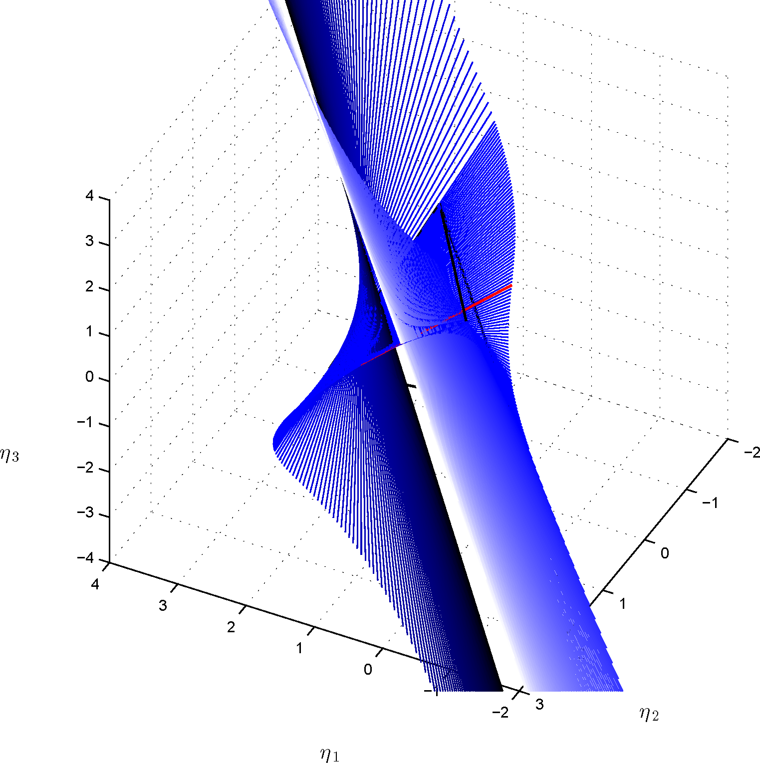
In Figures 6 and 7, we represent the extension of the ruled surface outside the probability simplex and in the (α, t) chart, while in Figures 8 and 9, the extended surface has been represented in the full marginal polytope parametrized by (η₁, η₂, η₃) and in the marginal polytope parametrized by (η₁, η₂).

3.4. Optimization and Natural Gradient Flows

We are interested in the study of natural gradient flows of functions defined over statistical models. Our motivation is the study of the optimization of the stochastic relaxation of a function, i.e., the optimization of the expected value of the function itself with respect to a distribution p in a statistical model. Natural gradient flows associated with the stochastic relaxation converge to the boundary of the model, where the probability mass is concentrated on some instances of the search space. To study the convergence over the boundary, we proposed to extend the natural gradient field outside the marginal polytope and the probability simplex, by employing a parameterization that describes the model as a ruled surface, as we described in the tutorial example of this section.

In the following, we focus on the optimization of a function f : Ω → ℝ, and we consider its stochastic relaxation with respect to a probability distribution in the exponential family in Equations (12) and (13). First, we compute a basis for all real-valued functions defined over Ω using algebraic arguments. Consider the zero-dimensional ideal I associated with the set of points in Ω, and let R be the polynomial ring with the field of real coefficients; a vector space basis for the quotient ring R/I defines a basis for all functions defined over Ω. In CoCoA [36], this can be computed with the command QuotientBasis.

Coming back to our example, with Ω = {1, 2, 3, 4}, by fixing the graded reverse lexicographical monomial order, which is the default one in CoCoA [36], we obtain a basis given by {1, x₁, x₂, x₁ x₂}, so that any f : Ω → ℝ can be written as:

$$f=c_0+c_1{x}_1+c_2{x}_2+c_{12}{x}_1{x}_2.$$

(61)

We are interested in the study of the natural gradient field of $F(p)={\mathbb{E}}_p[f]$. Recall that T₃ = 4x₁ + 3x₂ − 5x₁x₂ − 2 and ${\eta }_3=\mathbb{E}[{\mathrm{T}}_3]$, so that:

$$\mathbb{E}\left[x_1{x}_2\right]=\frac{1}{5}(4{\eta }_1+3{\eta }_2-{\eta }_3-2),$$

(62)

which implies:

$$F_{\eta }(\mathit{\eta })c_0-\frac{2}{5}{c}_{12}+\left(c_1+\frac{4}{5}{c}_{12}\right){\eta }_1+\left(c_2+\frac{3}{4}{c}_{12}\right){\eta }_2-\frac{1}{5}{c}_{12}{\eta }_3.$$

(63)

In order to study the gradient field of F_η(η) over the marginal polytope parameterized by (η₁, η₂), we need to express η₃ as a function of η₁ and η₂. In order to do that, we parametrize the exponential family as a ruled surface by means of the (α, t) parameters. Moreover, this parametrization has a natural extension outside the marginal polytope, which allows one to study the stability of the critical points on the boundary of the marginal polytope. We start by evaluating the gradient field of F_α,t(α, t) in the (α, t) parametrization, then we map it to the marginal polytope in the η parameterization.

By expressing (η₁, η₂) as a function of (α, t), we obtain:

$$F_{\alpha ,t}(\alpha ,t)=\frac{2{\alpha }^2(c_1+c_{12})+(2{\alpha }^2+2\alpha +1)(c_0+c_2)-(2{\alpha }^2(c_1+c_{12})+(2{\alpha }^2+2\alpha +1)(c_1\alpha +c_2))t}{2{\alpha }^2+2\alpha +1}.$$

(64)

If we take partial derivatives of Equation (64) with respect to α and t, we have:

$${\partial }_{\alpha }{F}_{\alpha ,t}(\alpha ,t)=\frac{4({\alpha }^2+\alpha )(c_1+c_{12})-((4{\alpha }^4+8{\alpha }^3+12{\alpha }^2+8\alpha +1)c_1+4({\alpha }^2+\alpha )c_{12})t}{4{\alpha }^4+8{\alpha }^3+8{\alpha }^2+4\alpha +1},$$

(65)

$${\partial }_t{F}_{\alpha ,t}(\alpha ,t)=-\frac{2{\alpha }^2{c}_{12}+(2{\alpha }^3+4{\alpha }^2+\alpha )c_1+(2{\alpha }^2+2\alpha +1)c_2}{2{\alpha }^2+2\alpha +1}.$$

(66)

In the (α, t) parameterization, the Fisher information matrix reads:

$$I_{\alpha ,t}(\alpha ,t)={\mathbb{E}}_{\alpha ,t}[-{\partial }^2\log p(x;\alpha ,t)]=\left[\begin{array}{cc}\frac{4{\alpha }^2-(4{\alpha }^4+8{\alpha }^3+12{\alpha }^2+8\alpha +1)t+4\alpha }{4{\alpha }^6+12{\alpha }^5+16{\alpha }^4+12{\alpha }^3+5{\alpha }^2+\alpha }& 0\\ 0& -{(t^2-t)}^{-1}\end{array}\right].$$

(67)

Finally, the natural gradient becomes:

$$\begin{array}{l}\tilde{\nabla }{F}_{\alpha ,t}(\alpha ,t)=I_{\alpha ,t}{(\alpha ,t)}^{-1}\nabla F_{\alpha ,t}(\alpha ,t)\\ =\left[\begin{array}{c}\frac{(4{\alpha }^6+12{\alpha }^5+16{\alpha }^4+12{\alpha }^3+5{\alpha }^2+\alpha )(4({\alpha }^2+\alpha )c_1+4({\alpha }^2+\alpha )c_{12}-((4{\alpha }^4+8{\alpha }^3+12{\alpha }^2+8\alpha +1)c_1+4({\alpha }^2+\alpha )c_{12})t)}{(4{\alpha }^4+8{\alpha }^3+8{\alpha }^2+4\alpha +1)(4{\alpha }^2-(4{\alpha }^4+8{\alpha }^3+12{\alpha }^2+8\alpha +1)t+4\alpha }\\ \frac{(2{\alpha }^2{c}_{12}+(2{\alpha }^3+4{\alpha }^2+\alpha )c_1+(2{\alpha }^2+2\alpha +1)c_2)(t^2-t)}{2{\alpha }^2+2\alpha +1}\end{array}\right]\end{array}$$

(68)

We obtained a rational formula for the natural gradient in the (α, t) parameterization, which can be easily extended outside the marginal polytope. However, notice that the inverse Fisher information matrix and the natural gradient are not defined for:

$$t=\frac{4({\alpha }^2+\alpha )}{4{\alpha }^4+8{\alpha }^3+12{\alpha }^2+8\alpha +1}.$$

(69)

We also remark that over the boundary of the model, for t ∈ {0, 1} and α ∈ {−1, 0}, the determinant of the inverse Fisher information vanishes, so that the matrix is not full rank. It follows that the trajectories associated with natural gradient flows with initial conditions in the interior of the marginal polytope remain in the marginal polytope.

In order to study the natural gradient field over the marginal polytope, we apply a reparameterization of a tangent vector from the (α, t) parameterization to the (η₁, η₂) parameterization. Indeed, by the chain rule and the inverse function theorem, we have:

$$\nabla F_{\eta }(\alpha ,t)=\nabla F_{\alpha ,t}{(\alpha ,t)}^{T}J{(\alpha ,t)}^{-1}$$

(70)

The Jacobian of the map (α, t) 7↦ (η₁, η₂) is:

$$J(\alpha ,t)=\left[\begin{array}{cc}-\frac{(6{\alpha }^2+8\alpha +1)t-4\alpha }{2{\alpha }^2+2\alpha +1}-\frac{2(2{\alpha }^2-(2{\alpha }^3+4{\alpha }^2+\alpha )t)(2\alpha +1)}{{(2{\alpha }^2+2\alpha +1)}^2}& -\frac{2{\alpha }^3+4{\alpha }^2+\alpha }{2{\alpha }^2+2\alpha +1}\\ 0& -1\end{array}\right],$$

(71)

with inverse:

$$J{(\alpha ,t)}^{-1}=\left[\begin{array}{cc}\frac{4{\alpha }^4+8{\alpha }^3+8{\alpha }^2+4\alpha +1}{4{\alpha }^2-(4{\alpha }^4+8{\alpha }^3+12{\alpha }^2+8\alpha +1)t+4\alpha }& \frac{4{\alpha }^5+12{\alpha }^4+12{\alpha }^3+6{\alpha }^2+\alpha }{4{\alpha }^2-(4{\alpha }^4+8{\alpha }^3+12{\alpha }^2+8\alpha +1)t+4\alpha }\\ 0& -1\end{array}\right].$$

(72)

It follows that:

$$\nabla F_{\eta }(\alpha ,t)=\left[\begin{array}{c}\frac{4({\alpha }^2+\alpha )c1+4({\alpha }^2+\alpha )c12-((4{\alpha }^4+8{\alpha }^3+12{\alpha }^2+8\alpha +1)c1+4({\alpha }^2+\alpha )c12)t}{4{\alpha }^2-(4{\alpha }^4+8{\alpha }^3+12{\alpha }^2+8\alpha +1)t+4\alpha }\\ -\frac{4({\alpha }^3+{\alpha }^2)c12-4({\alpha }^2+\alpha )c2+(2(2{\alpha }^4-{\alpha }^2)c12+(4{\alpha }^4+8{\alpha }^3+12{\alpha }^2+8\alpha +1)c2)t}{4{\alpha }^2-(4{\alpha }^4+8{\alpha }^3+12{\alpha }^2+8\alpha +1)t+4\alpha }\end{array}\right].$$

(73)

Notice that, as for the inverse Fisher information matrix, the inverse Jacobian J(α, t)⁻¹ is not defined for t which satisfies Equation (69).

We compute the inverse Fisher information matrix by evaluating the covariance between the sufficient statistics of the exponential family. Since over Ω, we have $x_1^2=x_1+x_1{x}_2$ and $x_1^2=x_1$, it follows that:

$$I_{\eta }{(\eta )}^{-1}=\left[\begin{array}{cc}\frac{1}{5}(9{\eta }_1+3{\eta }_2-{\eta }_3-2)-{\eta }_1^2& \frac{1}{5}(4{\eta }_1+3{\eta }_2+{\eta }_3-2)-{\eta }_1{\eta }_2\\ \frac{1}{5}(4{\eta }_1+3{\eta }_2-{\eta }_3-2)-{\eta }_1{\eta }_2& {\eta }_2-{\eta }_2^2\end{array}\right].$$

(74)

By parameterizing $I_{\eta }^{-1}$ with (α, t), we have:

$$\begin{array}{l}{I}_{\eta }{(\alpha ,t)}^{-1}\\ =\left[\begin{array}{cc}\frac{4{\alpha }^4+8{\alpha }^3-(4{\alpha }^6+16{\alpha }^5+20{\alpha }^4+8{\alpha }^3+{\alpha }^2)t^2+4{\alpha }^2+(4{\alpha }^5-12{\alpha }^3-8{\alpha }^2-\alpha )t}{4{\alpha }^4+8{\alpha }^3+8{\alpha }^2+4\alpha +1}& \frac{(2{\alpha }^3+4{\alpha }^2+\alpha )t^2-(2{\alpha }^3+4{\alpha }^2+\alpha )t}{2{\alpha }^2+2\alpha +1}\\ -\frac{(2{\alpha }^3+4{\alpha }^2+\alpha )t^2-(2{\alpha }^3+4{\alpha }^2+\alpha )t}{2{\alpha }^2+2\alpha +1}& -t^2+t\end{array}\right].\end{array}$$

(75)

Finally, we derive the following rational formula for the natural gradient over the marginal polytope parametrized as a ruled surface by (α, t):

$$\begin{array}{l}\tilde{\nabla }{F}_{\eta }(\alpha ,t)=I_{\eta }{(\alpha ,t)}^{-1}\nabla F_{\eta }(\alpha ,t)\\ =\left[\begin{array}{c}((4{\alpha }^6+16{\alpha }^5+20{\alpha }^4+8{\alpha }^3+{\alpha }^2)c_1+2(2{\alpha }^5+4{\alpha }^4+{\alpha }^3)c_{12}+(4{\alpha }^5+12{\alpha }^4+12{\alpha }^3+6{\alpha }^2+\alpha )c_2)t^2-4({\alpha }^4+2{\alpha }^3+{\alpha }^2)c_1+\\ -\frac{-4({\alpha }^4+2{\alpha }^3+{\alpha }^2)c_{12}-((4{\alpha }^5-12{\alpha }^3-8{\alpha }^2-\alpha )c_1+2(2{\alpha }^5+2{\alpha }^4-3{\alpha }^3-2{\alpha }^2)c_{12}+(4{\alpha }^5+12{\alpha }^4+12{\alpha }^3+6{\alpha }^2+\alpha )c_2)t}{4{\alpha }^4+8{\alpha }^3+8{\alpha }^2+4\alpha +1}\\ -\frac{(2{\alpha }^2{c}_{12}+(2{\alpha }^3+4{\alpha }^2+\alpha )c_1+(2{\alpha }^2+2\alpha +1)c_2)t^2-(2{\alpha }^2{c}_{12}+(2{\alpha }^2{c}_{12}+(2{\alpha }^3+4{\alpha }^2+\alpha )c_1+(2{\alpha }^2+2\alpha +1)c_2)t}{2{\alpha }^2+2\alpha +1}\end{array}\right].\end{array}$$

(76)

3.5. Examples with Global and Local Optima

We conclude this section with two examples of natural gradient flows associated with two different f functions. First, consider the case where c₀ = 0, c₁ = 1, c₂ = 2, c₃ = 3, so that:

$$\begin{array}{llll}\mathrm{\Omega }\hfill & x_1\hfill & x_2\hfill & f_1\hfill \\ 1\hfill & 0\hfill & 0\hfill & 0\hfill \\ 2\hfill & 0\hfill & 1\hfill & 2\hfill \\ 3\hfill & 1\hfill & 0\hfill & 1\hfill \\ 4\hfill & 2\hfill & 1\hfill & 10\hfill \end{array}.$$

(77)

The function admits a minimum on {1}. In Figure 10, we plotted the vector fields associated with the vanilla and natural gradient, together with some gradient flows for different initial conditions, in the (α, t) parameterization. In Figure 11, we represent the vanilla and natural gradient field over the marginal polytope in the (η₁, η₂) parameterization. Notice that, as expected, differently from the vanilla gradient, the natural gradient flows converge to the unique global optima, which corresponds to the vertex where all of the probability is concentrated over {1}. In the (α, t) parameterization, the flows have been extended outside the statistical model by prolonging the lines of the ruled surface, and as we can see, they remain compatible with the flows on the interior of the model, in the sense that the nature of the critical point is the same for trajectories with initial conditions on the interior and on the exterior of the model. In other words, the global optima is an attractor from both the interior and the exterior of the model and similarly for the other critical points on the vertices, both for saddle points and the unstable points, where the natural gradient vanishes.

In the second example, we set c₀ = 0, c₁ = 1, c₂ = 2, c₃ = −5/2, and we have:

$$\begin{array}{llll}\mathrm{\Omega }\hfill & x_1\hfill & x_2\hfill & f_2\hfill \\ 1\hfill & 0\hfill & 0\hfill & 0\hfill \\ 2\hfill & 0\hfill & 1\hfill & 2\hfill \\ 4\hfill & 2\hfill & 1\hfill & -1\hfill \\ \hfill & \hfill & \hfill & \hfill \end{array}$$

(78)

so that f₂ admits a minimum on {4}. In Figures 12 and 13, we plotted the vector fields associated with the vanilla and natural gradient, together with some gradient flows for different initial conditions, in the (α, t) and (η₁, η₂) parameterization, respectively. As in the previous example, natural gradient flows converge to the vertices of the model; however, in this case, we have one local optima in {1} and one global optima in {4}, together with a saddle point in the interior of the model. Similarly to the previous example, in the (α, t) parameterization, the flows have been extended outside the statistical model, and the nature of the critical points is the same for trajectories with initial conditions in the statistical model and in the extension of the statistical model.

We conclude the section by noticing that in both examples, for certain values of t in Equation (69), the natural gradient flows are not defined on the extension of the statistical model. As represented in the figures, once a trajectory encounters the dashed blue line in the (α, t) parameterization, the flow stops at that point.

4. Pseudo-Boolean Functions

We turn to discuss a case of considerable practical interest to see which of the results obtained in the example of the previous section we are able to extend.

For binary variables, we use the coding ±1, that is x = (x₁,…,x_n) ∈ {+1, −1}ⁿ = Ω. For any function f : Ω ↦ ℝ, with multi-index notation, f(x) = ∑_α∈L a_αx^α, with L = {0, 1}ⁿ and ${\mathit{x}}^{\alpha }={\displaystyle {\prod }_{i=1}^n{x}_i^{{\alpha }_i}}$, 0⁰=1. If M ⊂ L* = L\{0}, the model where p ∈ ε if:

$$p\propto \exp \left({\displaystyle \sum _{\alpha \in M}{\theta }_{\alpha }{X}^{\alpha }}\right)={{\displaystyle \prod _{\alpha \in M}\left(e^{{\theta }_{\alpha }}\right)}}^{X^{\alpha }}$$

has been considered in a number of papers on combinatorial optimization; see [3–5]. The following statements are results in algebraic statistics; cf. [20,35]. Let ${\mathcal{P}}^1=\{f\in {ℝ}^{\mathrm{\Omega }}|{\displaystyle {\sum }_{x\in \mathrm{\Omega }}p(\mathit{x})=1\}}$.

Proposition 6 (Implicitization of the exponential family). Given a function p: Ω → ℝ, then and p ∈ ε if, and only if, the following conditions all hold:

• p(x) > 0, x ∈ Ω;
• ∑_x∈Ωp(x)=1;
• ${\displaystyle {\prod }_{\mathit{x}:{\mathit{x}}^{\beta }=1}p\left(\mathit{x}\right)}={\displaystyle {\prod }_{\mathit{x}:{\mathit{x}}^{\beta }=-1}p\left(\mathit{x}\right)}$ for all β ∈ L*\M.

Proof. (⇒) If p ∈ ε, then p(x) > 0, x ∈ Ω (Item 1) and ∑_x∈Ω p(x) = 1 (Item 2). Moreover, log $p(\mathit{x})={\displaystyle {\sum }_{\alpha \in M}{\theta }_{\alpha }{\mathit{x}}^{\alpha }-\psi (\mathit{\theta })}$. The function log p is orthogonal to each X^β, β ∈ L* \ M. Hence:

$$0={\displaystyle \sum _{x\in \mathrm{\Omega }}\log p(\mathit{x}){\mathit{x}}^{\beta }}={\displaystyle \sum _{\mathit{x}:{\mathit{x}}^{\beta }=1}\log p\left(\mathit{x}\right)-}{\displaystyle \sum _{\mathit{x}:{\mathit{x}}^{\beta }=-1}\log p\left(\mathit{x}\right)}=\log {\displaystyle \prod _{\mathit{x}:{\mathit{x}}^{\beta }=1}p\left(\mathit{x}\right)}-\log {\displaystyle \prod _{\mathit{x}:{\mathit{x}}^{\beta }=1}p\left(\mathit{x}\right)},$$

(79)

which is equivalent to Item 3.

(⇐) Oppositely, the computation in Equation (79) implies that log p is orthogonal to each X^β; hence, there exists θ, such that log $p={\displaystyle {\sum }_{\alpha \in M}{\theta }_{\alpha }{\mathit{X}}^{\alpha }+C}$. Now, Item 2 implies C = −ψ(θ).

Let ℝ [Ω] denote the ring of polynomials in the indeterminates {p(x)|x ∈ Ω}. Given a binary model M, the set of polynomials:

$$\left\{{\displaystyle \prod _{\mathit{x}:{\mathit{x}}^{\beta }=1}p(\mathit{x})}-{\displaystyle \prod _{\mathit{x}:{\mathit{x}}^{\beta }=-1}p(\mathit{x})}|\beta \in L*\backslash M\right\},$$

generates an ideal $\mathcal{J}(M)$, which is called the toric ideal of the model M. Its variety $\mathrm{V}(M)$ is called the exponential variety of M.

Proposition 7.

• The exponential variety of M is the Zariski closure of the exponential model ε.
• The closure$\overline{ℰ}$ of ε in $\mathcal{P}\ge$ is characterized by p(x) ≥ 0, x ∈ Ω, together with Items 2 and 3 of Proposition 6.
• The algebraic variety of the ring ℝ[p(x): x ∈ Ω], which is generated by the polynomials Σ_x∈Ωp(x)−1, ${\displaystyle {\prod }_{\mathit{x}:{\mathit{x}}^{\beta }=1}p\left(\mathit{x}\right)}-{\displaystyle {\prod }_{\mathit{x}:{\mathit{x}}^{\beta }=-1}p\left(\mathit{x}\right)}$, β ∈ L* \ M, is an extension ε¹ of ε to ${\mathcal{P}}^1$.
• Define the moments${\eta }_{\alpha }={\displaystyle {\sum }_{\mathit{x}\in \mathrm{\Omega }}{\mathit{x}}^{\alpha }}p\left(\mathit{x}\right)$, α ∈ L, i.e., the discrete Fourier transform of p, with inverse$p(\mathit{x})=2^{-n}{\displaystyle {\sum }_{\alpha \in L}{\mathit{x}}^{\alpha }{\eta }_{\alpha }}$. There exists an algebraic extension of the moment function ε ∋ p ↔ η(p) ∈ M° to a mapping defined on ε¹.
• Proof. 1. According to the implicitization Proposition 6, the exponential family is characterized by the positivity condition together with the algebraic binomial conditions.
• This follows from the implicit form, and it is proven, for example, in [20].
• By definition.
• As the mapping from the probabilities to the moments is affine and one-to-one, such a transformation extends to a one-to-one mapping from the extended model to the affine space of the marginal polytope.

We conclude this section by introducing the so-called no three-way interaction example. On Ω = {0, 1}³, the full model in the statistics 0 ↦ 1, 1 ↦ −1, that is t = (−1)^x = 1 − 2x, is described by the matrix:

$$\begin{array}{l}1T_3{T}_2{T}_2{T}_3{T}_1{T}_1{T}_3{T}_1{T}_2{T}_1{T}_2{T}_3\\ D_3=\begin{array}{l}000\hfill \\ 001\hfill \\ 010\hfill \\ 011\hfill \\ 100\hfill \\ 101\hfill \\ 110\hfill \\ 111\hfill \end{array}\left[\begin{array}{llllllll}1\hfill & 1\hfill & 1\hfill & 1\hfill & 1\hfill & 1\hfill & 1\hfill & 1\hfill \\ 1\hfill & -1\hfill & 1\hfill & -1\hfill & 1\hfill & -1\hfill & 1\hfill & -1\hfill \\ 1\hfill & 1\hfill & -1\hfill & -1\hfill & 1\hfill & 1\hfill & -1\hfill & -1\hfill \\ 1\hfill & -1\hfill & -1\hfill & 1\hfill & 1\hfill & -1\hfill & -1\hfill & 1\hfill \\ 1\hfill & 1\hfill & 1\hfill & 1\hfill & -1\hfill & -1\hfill & -1\hfill & -1\hfill \\ 1\hfill & -1\hfill & 1\hfill & -1\hfill & -1\hfill & 1\hfill & -1\hfill & 1\hfill \\ 1\hfill & 1\hfill & -1\hfill & -1\hfill & -1\hfill & -1\hfill & 1\hfill & 1\hfill \\ 1\hfill & -1\hfill & -1\hfill & 1\hfill & -1\hfill & 1\hfill & 1\hfill & -1\hfill \end{array}\right].\end{array}$$

(80)

Note the lexicographic order of both the sample points and the statistics’ exponents.

The exponential family without the interaction term T₁T₂T₃ is the same model as the toric model without the three-way interaction, which is based on the matrix:

$$\begin{array}{l}C{\varsigma }_1{\varsigma }_2{\varsigma }_3{\varsigma }_4{\varsigma }_5{\varsigma }_6\\ B=\begin{array}{l}000\hfill \\ 001\hfill \\ 010\hfill \\ 011\hfill \\ 100\hfill \\ 101\hfill \\ 110\hfill \\ 111\hfill \end{array}\left[\begin{array}{lllllll}1\hfill & 0\hfill & 0\hfill & 0\hfill & 0\hfill & 0\hfill & 0\hfill \\ 1\hfill & 1\hfill & 0\hfill & 1\hfill & 0\hfill & 1\hfill & 0\hfill \\ 1\hfill & 0\hfill & 1\hfill & 1\hfill & 0\hfill & 0\hfill & 1\hfill \\ 1\hfill & 1\hfill & 1\hfill & 0\hfill & 0\hfill & 1\hfill & 1\hfill \\ 1\hfill & 0\hfill & 0\hfill & 0\hfill & 1\hfill & 1\hfill & 1\hfill \\ 1\hfill & 1\hfill & 0\hfill & 1\hfill & 1\hfill & 0\hfill & 1\hfill \\ 1\hfill & 0\hfill & 1\hfill & 1\hfill & 1\hfill & 1\hfill & 0\hfill \\ 1\hfill & 1\hfill & 1\hfill & 0\hfill & 1\hfill & 0\hfill & 0\hfill \end{array}\right]\end{array}$$

(81)

that is the probabilities as a function of the ζ’s are:

$$\{\begin{array}{l}{p}_1=c\\ p_2=c{\varsigma }_1{\varsigma }_3{\varsigma }_5\\ p_3=c{\varsigma }_2{\varsigma }_3{\varsigma }_6\\ p_4=c{\varsigma }_1{\varsigma }_2{\varsigma }_5{\varsigma }_6\\ p_5=c{\varsigma }_4{\varsigma }_5{\varsigma }_6\\ p_6=c{\varsigma }_1{\varsigma }_3{\varsigma }_4{\varsigma }_6\\ p_7=c{\varsigma }_2{\varsigma }_3{\varsigma }_4{\varsigma }_5\\ p_8=c{\varsigma }_1{\varsigma }_2{\varsigma }_4\end{array}.$$

(82)

The toric ideal of the toric model in Equation (82) is generated by the polynomial:

$$p_2{p}_3{p}_5{p}_8-p_1{p}_4{p}_6{p}_7=0,$$

(83)

this means that the closure of the exponential family is given by the solution of the equations:

$$\{\begin{array}{l}{p}_1+p_2+p_3+p_4+p_5+p_6+p_7+p_8=1\\ p_2{p}_3{p}_5{p}_8-p_1{p}_4{p}_6{p}_7=0\end{array}.$$

(84)

The η parameters are the expected values of the sufficient statistics of the full model,

$$\begin{array}{l}000001010011100101110111\\ \left[\begin{array}{l}{\eta }_1\hfill \\ {\eta }_2\hfill \\ {\eta }_3\hfill \\ {\eta }_4\hfill \\ {\eta }_5\hfill \\ {\eta }_6\hfill \\ {\eta }_7\hfill \end{array}\right]=\left[\begin{array}{l}001\hfill \\ 010\hfill \\ 011\hfill \\ 100\hfill \\ 101\hfill \\ 110\hfill \\ 111\hfill \end{array}\right]\left[\begin{array}{llllllll}1\hfill & -1\hfill & 1\hfill & -1\hfill & 1\hfill & -1\hfill & 1\hfill & -1\hfill \\ 1\hfill & 1\hfill & -1\hfill & -1\hfill & 1\hfill & 1\hfill & -1\hfill & -1\hfill \\ 1\hfill & -1\hfill & -1\hfill & 1\hfill & 1\hfill & -1\hfill & -1\hfill & 1\hfill \\ 1\hfill & 1\hfill & 1\hfill & 1\hfill & -1\hfill & -1\hfill & -1\hfill & -1\hfill \\ 1\hfill & -1\hfill & 1\hfill & -1\hfill & -1\hfill & 1\hfill & -1\hfill & 1\hfill \\ 1\hfill & 1\hfill & -1\hfill & -1\hfill & -1\hfill & -1\hfill & 1\hfill & 1\hfill \\ 1\hfill & -1\hfill & -1\hfill & 1\hfill & -1\hfill & 1\hfill & 1\hfill & -1\hfill \end{array}\right]\left[\begin{array}{l}{p}_1\hfill \\ p_2\hfill \\ p_3\hfill \\ p_4\hfill \\ p_5\hfill \\ p_6\hfill \\ p_7\hfill \\ p_8\hfill \end{array}\right].\end{array}$$

(85)

In the ring:

$$R=\mathbb{Q}[p_1,p_2,p_3,p_4,p_5,p_6,p_7,p_8,{\eta }_2,{\eta }_3,{\eta }_4,{\eta }_5,{\eta }_6,{\eta }_7]$$

(86)

we can consider the ideal $\mathrm{I}$ generated by the Equations (84) together with Equations (85). The elimination ideal:

$$\mathcal{J}=\mathrm{I}\cap \mathbb{Q}[{\eta }_1,{\eta }_2,{\eta }_3,{\eta }_4,{\eta }_5,{\eta }_6,{\eta }_7]$$

(87)

will express the model as a dependence between the η’s.

Computation with CoCoA [36] gives the following polynomial:

$$\begin{array}{l}f\left({\eta }_1,{\eta }_2,{\eta }_3,{\eta }_4,{\eta }_5,{\eta }_6;{\eta }_7\right)=\\ {\eta }_1^2{\eta }_3{\eta }_4+{\eta }_2^2{\eta }_3{\eta }_4-{\eta }_3^3{\eta }_4-{\eta }_3{\eta }_4^3+{\eta }_1^2{\eta }_2{\eta }_5-{\eta }_2^3{\eta }_5+{\eta }_2{\eta }_3^2{\eta }_5+{\eta }_2{\eta }_4^2{\eta }_5+{\eta }_3{\eta }_4{\eta }_5^2-{\eta }_2{\eta }_5^3-{\eta }_1^3{\eta }_6+{\eta }_1{\eta }_2^2{\eta }_6+{\eta }_1{\eta }_3^2{\eta }_6\\ +{\eta }_1{\eta }_4^2{\eta }_6+{\eta }_1{\eta }_5^2{\eta }_6+{\eta }_3{\eta }_4{\eta }_6^2+{\eta }_2{\eta }_5{\eta }_6^2-{\eta }_1{\eta }_6^3-2{\eta }_1{\eta }_2{\eta }_4-2{\eta }_1{\eta }_3{\eta }_5-2{\eta }_2{\eta }_3{\eta }_6-2{\eta }_4{\eta }_5{\eta }_6+{\eta }_3{\eta }_4+{\eta }_2{\eta }_5+{\eta }_1{\eta }_6\\ +\left(-2{\eta }_1{\eta }_2{\eta }_3-2{\eta }_1{\eta }_4{\eta }_5-2{\eta }_2{\eta }_4{\eta }_6-2{\eta }_3{\eta }_5{\eta }_6+{\eta }_1^2+{\eta }_2^2+{\eta }_3^2+{\eta }_4^2+{\eta }_5^2+{\eta }_6^2-1\right){\eta }_7\\ +\left({\eta }_3{\eta }_4+{\eta }_2{\eta }_5+{\eta }_1{\eta }_6\right){\eta }_7^2+\left(-1\right){\eta }_7^3.\end{array}$$

(88)

The equation:

$$f\left({\eta }_1,{\eta }_2,{\eta }_3,{\eta }_4,{\eta }_5,{\eta }_6;{\eta }_7\right)=0$$

(89)

is an expression of the model in the expectation parameters, and this expression is a polynomial equation. We know unique solvability in η₇ if (η₁, η₂, η₃, η₄, η₅, η₆) is in the interior of the marginal polytope. As in the example of the previous section, it is possible to intersect the polynomial invariant in Equation (83) with one or more sheaves of hyperplanes around some faces of the simplex, in order to lower the degree of the invariant and thus decompose the model as the convex hull of probabilities on the boundary of the model. We do not describe the details here, and we postpone the discussion of this example to a paper which is in preparation.

5. Conclusions

Geometry and algebra play a fundamental role in the study of statistical models, and in particular in the exponential family. In the fist part of the paper, starting from the definition of the natural gradient over an exponential family, we described the relationship between its expression in the basis of the sufficient statistics and in the conjugate basis. From this perspective, the terms natural gradient and vanilla gradient, to denote gradients evaluated with respect to the Fisher and the Euclidean geometry, together with their duality in the natural and expectation parameters, assume a new meaning, since these definitions depend on the choice of the basis for the tangent space.

In order to study natural gradient flows for a generic discrete exponential model and, in particular, their convergence, it is convenient to move to the mixture geometry of the expectation parameters and to study trajectories over the marginal polytope. However, in order to obtain explicit equations for the flows, it is necessary to determine the dependence between the moments associated with the sufficient statistics of the model, which are constrained to belong to the marginal polytope, and the remaining moments, which on the other side are not free. Such a relationship, which for finite search spaces is given by a system of polynomial invariants, cannot be easily solved explicitly in general. In the second part of the paper, by using algebraic tools, we proposed a novel parameterization based on ruled surfaces for an exponential family, which does not require to solve the polynomial invariant explicitly. We applied our approach to a simple example, and we showed that the surface associated with the model in the full marginal polytope is a ruled surface. We claim that these results are not peculiar to the example we described, and we are working towards an extension of this approach in a more general case.