
A Hybrid Physical and Maximum-Entropy Landslide Susceptibility Model

Department of Geography & Environment, San Francisco State University, 1600 Holloway Ave., San Francisco, CA 94132, USA
*
Author to whom correspondence should be addressed.
Entropy 2015, 17(6), 4271-4292; https://doi.org/10.3390/e17064271
Submission received: 28 February 2015
/
Revised: 28 May 2015
/
Accepted: 12 June 2015
/
Published: 19 June 2015
(This article belongs to the Special Issue Entropy in Hydrology)
Abstract
:The clear need for accurate landslide susceptibility mapping has led to multiple approaches. Physical models are easily interpreted and have high predictive capabilities but rely on spatially explicit and accurate parameterization, which is commonly not possible. Statistical methods can include other factors influencing slope stability such as distance to roads, but rely on good landslide inventories. The maximum entropy (MaxEnt) model has been widely and successfully used in species distribution mapping, because data on absence are often uncertain. Similarly, knowledge about the absence of landslides is often limited due to mapping scale or methodology. In this paper a hybrid approach is described that combines the physically-based landslide susceptibility model “Stability INdex MAPping” (SINMAP) with MaxEnt. This method is tested in a coastal watershed in Pacifica, CA, USA, with a well-documented landslide history including 3 inventories of 154 scars on 1941 imagery, 142 in 1975, and 253 in 1983. Results indicate that SINMAP alone overestimated susceptibility due to insufficient data on root cohesion. Models were compared using SINMAP stability index (SI) or slope alone, and SI or slope in combination with other environmental factors: curvature, a 50-m trail buffer, vegetation, and geology. For 1941 and 1975, using slope alone was similar to using SI alone; however in 1983 SI alone creates an Areas Under the receiver operator Curve (AUC) of 0.785, compared with 0.749 for slope alone. In maximum-entropy models created using all environmental factors, the stability index (SI) from SINMAP represented the greatest contributions in all three years (1941: 48.1%; 1975: 35.3; and 1983: 48%), with AUC of 0.795, 0822, and 0.859, respectively; however; using slope instead of SI created similar overall AUC values, likely due to the combined effect with plan curvature indicating focused hydrologic inputs and vegetation identifying the effect of root cohesion. The combined approach––using either stability index or slope––highlights the importance of additional environmental variables in modeling landslide initiation.
1. Introduction
Mass movement or mass wasting describes the movement of rock, debris, soil, or earth material by gravity. This movement may be fast or slow, typically depending on the amount of water present in the mass. Therefore multiple kinds of mass wasting can be distinguished. Varnes [1] has provided a comprehensive and widely accepted classification of mass movement types. Landslides are a special case of mass movement, but the term is also often used as a general description of any loose material sliding down a slope. The sizes of landslides vary, with smaller ones being more common than larger ones. Landslides are triggered when a threshold of stability is crossed, usually involving earthquakes or excess water, or an intrinsic threshold resulting from successive weathering of slope material [2]. Hydrologic inputs are a significant contributor to decreasing slope stability by their effect on pore pressure, and redirected flows can lead to slope failures. For instance, soil piping can contribute to landslides by increasing within-soil drainage rates [3], and runoff from impervious surfaces such as roads [4] can also contribute to downslope failures through concentrating flow.
Landslides can be a serious threat to human habitat, and they are amongst the most damaging geo-hazards, although their effect may be attributed to the triggering factor. Recently, the 2014 Oso landslide in Washington State, USA, likely due to prolonged precipitation and involving a volume of 8 × 10⁶ m3 over an area of about 2.6 km2, killed 41 people [5,6]. In 2010, a large landslide along the Hunza River in Pakistan not only erased two villages, but additionally created a large dam resulting in a lake which flooded villages upstream and threatened flooding of habitat downstream [7]. The cumulative effect of small landslides can also be very destructive, particularly when large regions are affected by swarms of landslides. Thousands of landslides caused by an intense storm in January of 1982 resulted in the loss of life of 25 people in the San Francisco Bay area. Although most of these slides were not of large size, some of the scars can still be recognized on recent aerial photography.
Given that landslides can be a dangerous event, it is important to understand their behaviour, and the conditions under which they occur. For this purpose, a spatiotemporal inventory of landslide episodes in the past is critical, and these inventories are a crucial component in the process of landslide analysis. Various methods are applied, although the most common procedures are identification in the field and detection of landslide scars from aerial photography. There are of course many logistical challenges in developing timely, accurate inventories; and it has been shown that landslide inventories can differ between investigators, methods applied, and multiple scales of data sources [8,9]. Recently, semi-automated landslide mapping using object-oriented image analysis (OBIA) from very-high resolution satellite images has received some attention [10,11]. Full automation has yet to be achieved, but this approach could be a promising path to rapidly creating a landslide record shortly after the event. The inventory is subsequently used to create maps of landslide susceptibility in order to identify areas or locations that may experience sliding at some time in the future. Landslide hazard maps finally combine spatial with temporal probabilities [6,9].
Landslide susceptibility mapping typically involves one of three approaches: heuristic reasoning, statistical analysis, and physically-based models. Each procedure has advantages and disadvantages. In general, heuristic methods are considered basic, involving coarse scales; statistical analysis is assumed to be appropriate at intermediate scales; while deterministic or physically-based methods are the most sophisticated but may only be possible at very fine scales. This progression from basic to sophisticate necessitates the inclusion of additional parameters. For example, physically-based models require geotechnical parameters, such as soil or root cohesion and angle of internal friction [12]. These variables are not routinely collected or available for large areas.
Heuristic models can be easily implemented in a GIS environment and include consideration of variables such as lithology, geomorphology, land use, soils, or elevation and its derivatives. It should be noted, however, that slope needs to be treated with caution at coarse scales. A more detailed discussion of the variables can be found in van Westen et al. [9]. These variables are frequently weighted either by the investigator, or by more objective methods, such as multi-criteria decision analysis or physical modeling [13,14].
Statistical models require a thorough landslide inventory for at least part of the study area for model development and validation. In addition, they assume that the environmental factors in the validation and development part of the study area are very similar. Statistical models that have been widely adopted to model landslide susceptibility are logistic regression and discriminant analysis [15]. While appealing and easily interpreted, these methods assume that the modeler has data on absences, which is unlikely to be true. Landslide inventories vary depending on scale or method, so that the absence of a landslide on a particular map may not necessarily imply that there are no landslides at a certain location. Only large-scale field-based methods have the potential to clearly show even smaller failures, whereas aerial photography-based methods may miss landslides due to vegetation cover or insufficient scale. Even so, older landslides may be fairly obscured due to erosional processes [8].
Physically-based models of landslides often employ the limit equilibrium method, predicting slope stability as a factor of safety (FS) from cohesion, slope, pore water pressure and angle of internal friction. The factor of safety describes the stability of a slope as a ratio of shear strength and shear stress. While methods to calculate the FS vary, in a GIS environment, the infinite slope method is used almost exclusively, because it is the most suitable for a pixel-based analysis. The factor of safety can be written as (modified after Tosi [16]):
where c′ is effective soil cohesion, γ is unit weight of the soil, z is soil depth, θ is slope angle, and ϕ is effective angle of internal friction.
Cohesion ideally includes the added effect of root cohesion, which can be complex with large ranges even within nominally forested land cover, because the cohesive action of roots will have a stabilizing effect on the slope to the point of preventing the slope from failure [16,17]. While root cohesion can be quantified, this is a complex procedure not routinely done and availability of sufficiently spatially accurate data is extremely limited. Although it is therefore often ignored, there have been instances where it is included. Attempts have been made to relate root cohesion to satellite derived vegetation information [18,19]. However, more research is needed in this area.
When studying large numbers of landslides in a study area with limited detailed geotechnical site data, statistical methods commonly provide higher prediction accuracies [20], though the results are best seen as identifying causal factors instead of a general model that can be applied to many sites as a physical model can be. Other methods such as support vector machine, artificial neural networks, fuzzy logic, or decision trees have also been successfully employed recently, including applications of hybrid or ensemble methods [14,21–23].
While classical entropy-based models have long been used in geomorphic systems (e.g., on longitudinal profiles and on stream morphology), application to event-based landforms such as landslides and gullies is recent, although Haigh [24] distinguished entropy dissipating and entropy accumulating landslides in the Himalayas. The presence-only nature of landslides––or the limited knowledge of absence locations––makes maximum entropy methods designed for species habitat analysis appealing. Geomorphological events such as rapid mass wasting share many characteristics with biological occurrences in that while they respond to environmental conditions, absences may not imply the lack of favorable conditions. At a local scale, positively and negatively spatially autocorrelated effects may also play a part, since mass wasting events may either increase the likelihood of other events in close proximity due to increasing hillslope gradients along the failure margins, or change the local hydrological conditions to decrease the probability for nearby events.
This research presents a novel hybrid or ensemble type model where the result of a physically-based method is incorporated into an entropy model, specifically a maximum entropy model (MaxEnt). Physical and maximum entropy models are at opposite ends of the spectrum in that the former is easily interpreted, based on physical principles, while the latter is in the realm of black boxes, operating in information (sometimes called environmental) space. However, the hybrid approach combines advantages of both methods. Given an appropriate scale of study where all critical parameters are known, physical models are clearly the best approach, and those that are spatially explicit should be able to have a high predictive power. However, many of these parameters are poorly known and spatially heterogeneous, so a pure physical modeling approach may be difficult to achieve. Maximum entropy models make no statistical assumptions about the variables used as inputs, and as a Bayesian approach focuses on maximizing probabilities, in this case that observations are similar based upon inputs in terms of maximizing entropy in information space which may include environmental space [25]. In the process, the model is parsimonious, with variables incorporated on the basis of their being necessary and sufficient in maximizing prediction accuracy [26].
2. Study Area
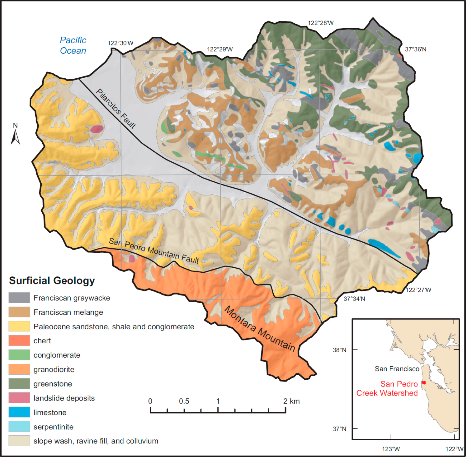
The 21.3 km2 watershed of San Pedro Creek (Pacifica, CA, USA) has been the focus of numerous landslide and hydrological studies as a result of its steep hillslopes and hazardous conditions [27]. Steep hillslopes are common with more than ten per cent of slopes greater than 35° and a median slope at 10 m precision of 21°. The maximum elevation is along the southern boundary of the watershed, the 578-m North Peak of Montara Mountain, a mass of granodiorite on the Salinian block that is moving northwestward with the Pacific Plate (Figure 1). The dominant surficial geology derives from marine deposits accreted at a convergent plate boundary, divided by the right-lateral Pilarcitos Fault into Jurassic/Cretaceous Franciscan Assemblage of graywacke, melange, greenstone, limestone and serpentinite to the north; and Paleogene marine sedimentary rocks to the south, including extensive uplifted turbidite beds visible along coastal bluffs. Mollisols of varying thickness have developed on weathered bedrock, slopewash, ravine fill and colluvium [28,29].
Land cover is one third urbanized as residential and commercial development, including most of the valley floors but extending upslope (Figure 2). The undeveloped areas are vegetated by a mixture of native and exotic grasses, forests, coastal scrub and chaparral, with riparian corridors of varying complexity along drainage lines (Figure 3). Upland vegetation communities are influenced by bedrock type, soil depth, slope and aspect, with Arctostaphylos chaparral prominent on steep areas with thin soils, and coastal scrub (with Baccharis pilularis, Chrysolepis chrysophylla, and other species) commonly on colluvium. Grasses are primarily on some south facing slopes, while trees are primarily introduced, mostly composed of Eucalyptus globulus and Pinus radiata.
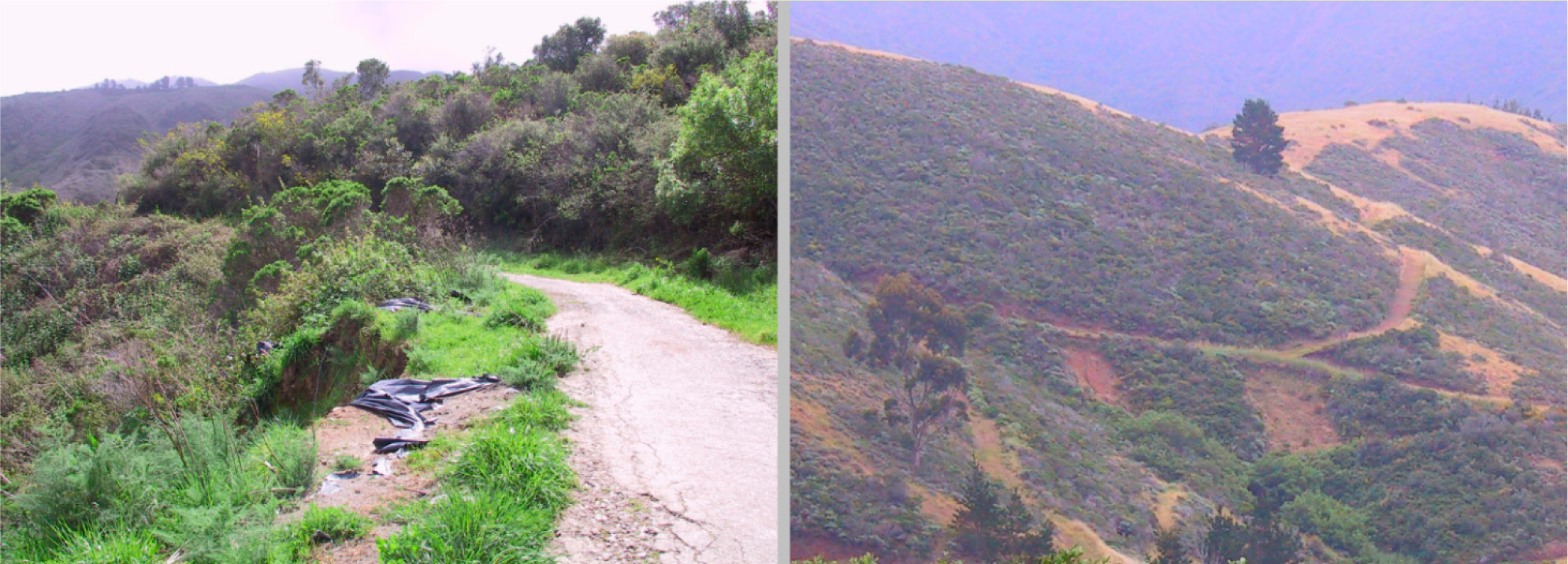
A combination of steep terrain and relatively weak bedrock can lead to extensive debris flows and slides during intense rainfall events [31]. Field and aerial photographic analysis conducted during a sediment source analysis [32] also points to the significance of impervious runoff from roads crossing steep midslopes, as seen in Figure 4. Precipitation is markedly seasonal, with 90% of the 840 mm annual rainfall occurring between November and April [33].
3. Methodology
3.1. Physically-Based Model
Several versions of the infinite slope method have been employed with two good examples being SHALSTAB and SINMAP [34]. For this research SINMAP was used where the FS is given as:
where C is made dimensionless by a combination of soil (Cs) and root cohesion (Cr), soil thickness D, soil density ρs, and gravity g.
Here, r = ρw/ρs is the ratio of the density of water to soil density, and the ratio of the height of the saturated zone, Dw, and D, is the relative wetness w = Dw/D.
The model extends the infinite slope model spatially to accumulate flows downslope, using the assumption that the capacity for downslope lateral flux is T sinθ, where T is soil transmissivity (m2 h−1) derived as the product of hydraulic conductivity and soil thickness, and provides spatial patterns of relative wetness. In SINMAP, together with an estimate of specific catchment area a = A/b, where A is contributing area for unit contour length b, slope and recharge (R) relative to transmissivity T, the relative wetness w is derived as:
A stability index (SI) is then derived as the minimum factor of safety, with minimum cohesion and maximum recharge-to-transmissivity ratio. For
, SI is set to
; and for
, SI is set to zero [34].
3.2. Maximum Entropy Model
Maximum entropy (MaxEnt) is increasingly being considered in the study of a variety of earth system processes [35,36]. MaxEnt compares the conditional density function of covariates (predictor variables) at presence sites
to the marginal (background) density of covariates in the study area
, in order to derive the conditional occurrence probability
[37]. Maximum entropy models derive from information theory (as opposed to thermodynamic entropy models), and have shown promise in a variety of applications in earth science [38].
A maximum entropy modeling approach was used by Convertino et al. [26] for the 9130 km2 Arno River basin in the Tuscany region of Italy. Felicísimo [39] compared logistic regression, the maximum entropy (MaxEnt) application of Phillips et al. [40], multiple adaptive regression splines (MARS), and classification and regression trees (CART) for modeling landslide susceptibility in a region of northern Spain; CART and MaxEnt performed best based upon area under the receiver operator characteristic curve (AUC).
3.3. Hybrid Model
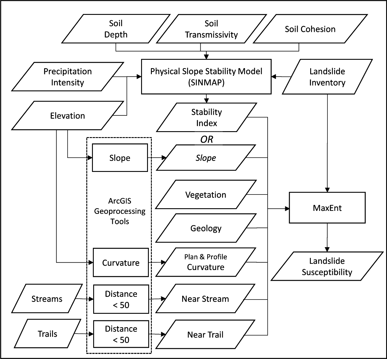
We propose a hybrid approach (Figure 5), starting with a physical infinite-slope model extended spatially with downslope accumulated flows influenced by soil thickness and tranmissivity (SINMAP) that is then used as an input into a maximum entropy model that is able to incorporate factors unsuitable for the physical model; various GIS geoprocessing tools are also used to create derivative datasets such as slope, curvature, and distances to streams and trails or roads. A physical model such as SINMAP has the advantage of employing the nature of water movement and the stability factors of the infinite slope model, and thus it can go farther than its inputs can do statistically, but it also has limitations. Inputs to the model itself are often difficult to assess, and cohesion in particular is well known to vary spatially, due in part to the major influence yet complex nature of root cohesion [41]. If no suitable root cohesion data are available, maps generated by the purely physical model considering only particle cohesion often show extensive slope failures. This is not surprising given the well-known counteracting role of root structures for preventing landslides. Because some parameters, particularly engineering properties of soil, such as cohesion and friction angle are difficult to quantify with the physically-based models at medium to coarse scales; other variables, such as distance to streams, roads and trails become more significant. Many slope failures may be attributed to local hydrologic factors such as concentrated runoff from impervious surfaces, for example trails and abandoned roads built on hillslopes. A hybrid approach incorporating as an input slope stability derived from a physical model, itself unattainable from any statistical approach, has the potential to do better than either a purely physical or purely statistical model.
3.4. Landslide Scar Data and Causal Factors
Landslides are commonly focused in colluvial hollows similar to those described by Reneau et al. [42], and in this watershed colluvial fills of up to 6 m have been documented [43]. Subsurface hydrology is a major cause of shallow landslides [44]. Landslides appear to largely originate on slopes of 26°–45° and more than 35% of all watershed hillslopes fall into this range. In an El Niño event of January 1982, the largest landslides all occurred between a narrow range of 26°–30° [45] during a period of intense rainfall on already saturated hillslopes [46].
Urbanization has been an important factor increasing landslide hazards in the watershed. Pampeyan [30] found that hillslope toe removal associated with increased development is a factor in increasing landslide potential within the watershed. Development on steep hillslopes has been seen as a contributing cause of landslides, leading in the 1970’s to the passage of a Hillside Protection Ordinance by the City of Pacifica. Finally, recreational use of steep hillslopes has led to the construction of extensive trail networks, most problematically in the case of off-road motorcycles, though the latter use has been greatly curtailed in recent decades. These trails divert and concentrate flow, contributing to landslide hazards downslope.
A combination of archival research, aerial photography interpretation and field surveys were used to compile a spatiotemporal inventory of landslides (as well as gullies) occurring in San Pedro Creek watershed [32]. In this study, shallow landslides were identified by scars and tracks from imagery from 1941 (1:24,000), 1955 (1:10,000), 1975, 1983, 1991 and 1997 (1:12,000). Environmental factors considered included surficial geology, vegetated land cover, distances to streams and trail networks, and slope and curvature derivatives of elevation. While gullies were primarily developed during the earlier agricultural development of the watershed, as seen on the 1941 aerial photograph, steep topography and intense rainfall events clearly drove the patterns of landslides especially in later years with an expansion of impervious surfaces including road and trail development on hillslopes [47]. The focus of this paper is on a hybrid model applied to data collected for these studies for 1941, 1975 and 1983, when contributing factors appear to be more closely aligned with either (a) expansion of agricultural and other land uses (1941 imagery), (b) hydrological connectivity to impervious surfaces (1975), or (c) widespread slope instability after an intense precipitation event in 1982 (1983).
Causal factors considered included categorical variables such as major vegetation classes (grassland/herbaceous, scrub, and forest), major surficial geology groups (granitics, sandstone, and colluvial hillslope deposits), and proximity to trails and streams. Vegetation is based on Wieslander [48] for 1941; aerial photographic interpretation in 1955, 1975, 1983, and 1997; and 2002 field mapping [49]. The most significant vegetation changes occurred between 1955 and 1975, a time of accelerated suburban development of the watershed. Trails and predominantly dirt roads built on hillslopes were digitized from these same aerial photographs (paved roads on valley floors were not used in our analysis.)
Continuous factors were derived from elevation data, including slope and curvature. We acquired elevation data in two resolutions––3 m from LiDAR and 10 m from photogrammetric contouring––from the US Geological Survey, but selected the 10-m data for the model to avoid detecting actual scars in the LiDAR data. Each source has characteristic artifacts––LiDAR noise and stepped contour interpolation effects––that were mitigated using 3 × 3 low-pass filters: one for slope and two in succession for curvature. Spatial variation in precipitation intensity as was used in Convertino et al. [26], was not considered for our study due to the relatively small size of our study area with very few rain gauges to derive a suitable spatial input. Categorical variables included vegetation, geology, and Boolean 50-m trail and stream buffers.
4. Results
The hybrid landslide susceptibility model (see Figure 5) starts with deriving a stability index that employs data on soils, surficial geology, and elevation. Transmissivity and soil thickness were derived from a combination of soil and colluvium thickness, and a single set of inputs to approximate two contrasting conditions that create similar SINMAP inputs was selected: (a) moderately thick soils with high hydraulic conductivity on the granitic slopes of Montara Mountain, and (b) deep colluvium with moderate hydraulic conductivity (Table 1). Steady-state rainfall conditions are assumed.
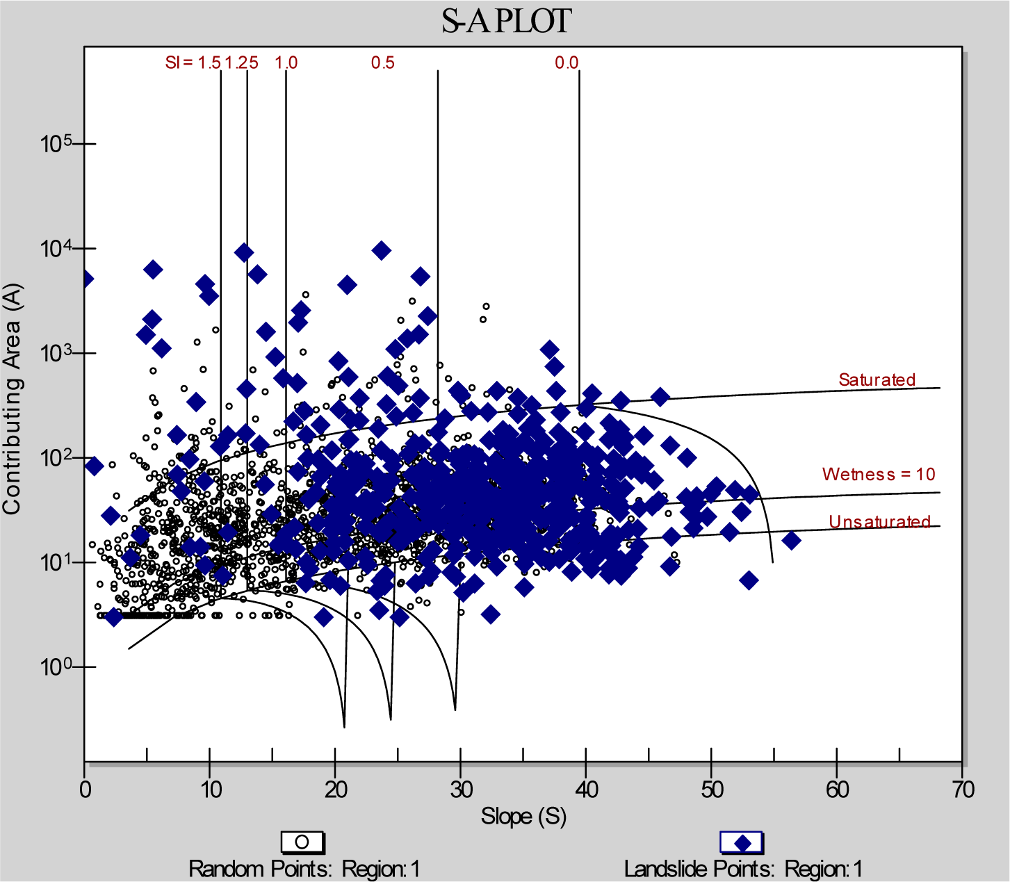
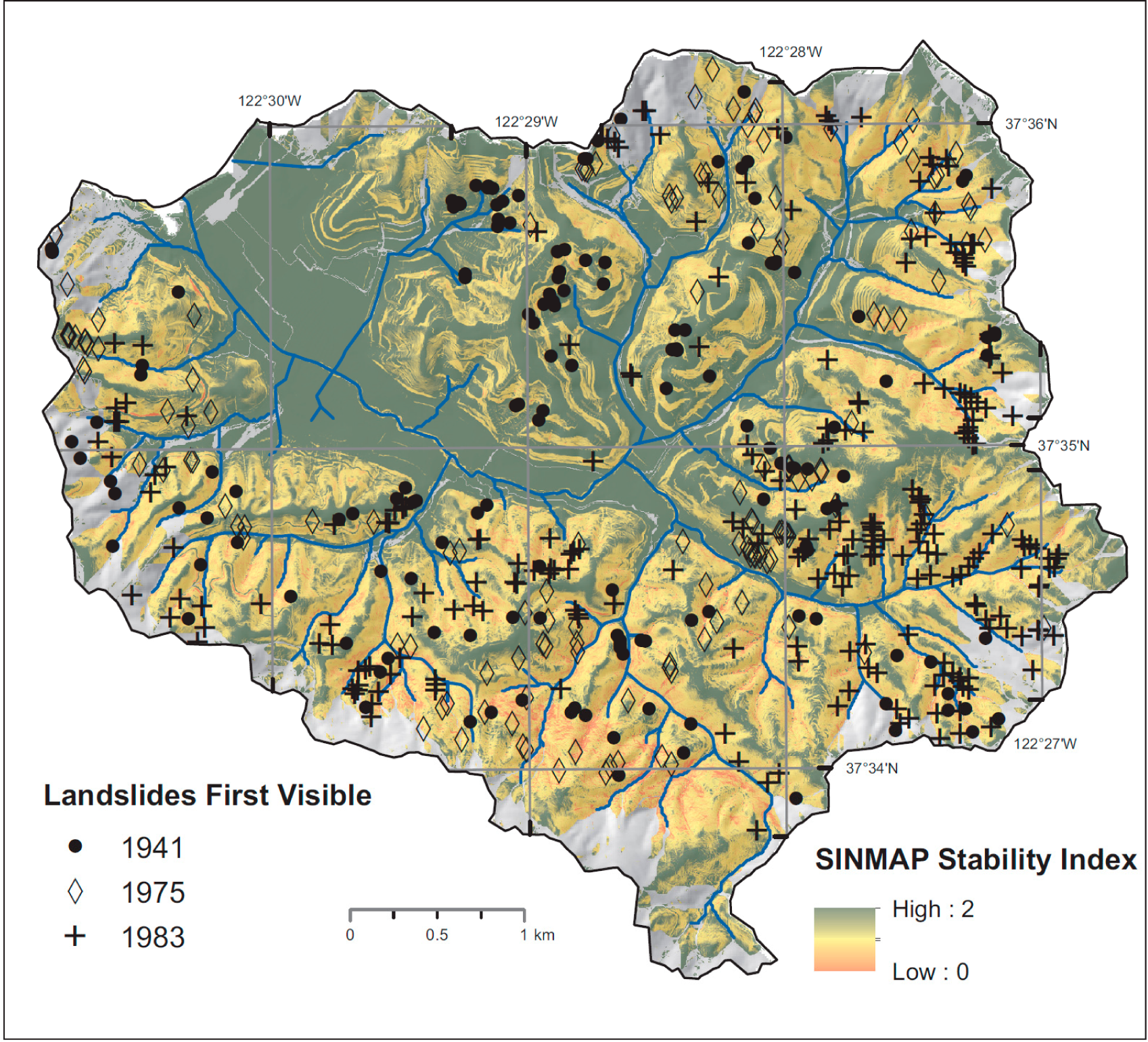
Given these assumptions, inventoried landslides from all years were predicted by SINMAP to be mostly undersaturated but unstable, with majorities of observed scars predicted in areas with a stability index less than 1.0 (Figure 6; Table 2). The stability index is mapped together with 1941, 1975, and 1983 landslides in Figure 7. The general patterns observed is a widespread occurrence of slope failures each year, with 154 visible in 1941, 142 in 1975 and 252 in 1983. The last period is strikingly missing scars on the steepest slopes of Montara Mountain, suggesting somewhat contrasting conditions for slope failures captured in 1983. In both 1975 and 1983, however, many areas with predicted low stability index experienced no landslides, and while this may partially relate to an inability to predict the more complex local hydrologic flow and cohesion patterns in soils and colluvium, clearly missing are some important spatial controls that could not be considered in the physical model.
Variations in root cohesion is clearly an important missing variable in the physical model. The SINMAP inputs were based on soil particle cohesion alone, yet it appears this is insufficient to avoid slope failure; this is not surprising as the significance of roots in maintaining slopes is well known [16]. Given the highly variable depth of rooting in general and for scrub and chaparral plant communities in particular, however, reasonable root cohesion estimates could not be sufficiently partitioned spatially to derive realistic estimates for physical modeling. Other potentially important variables may be slope curvature and proximity to features such as impervious surfaces and streams. In the hybrid model, the stability index result from SINMAP is therefore transferred along with these other factors into a maximum entropy model.
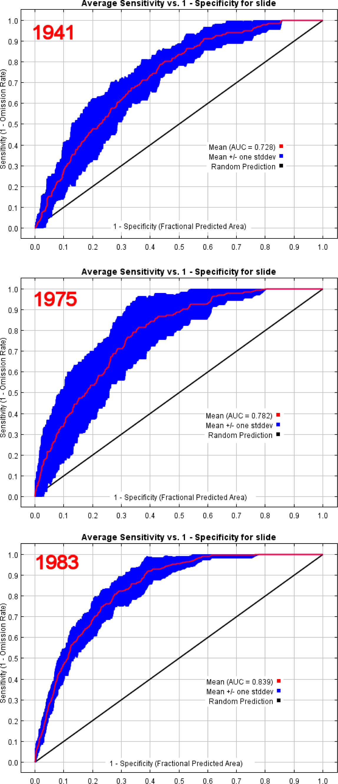
MaxEnt models were developed for landslides first visible in 1941, 1975, and 1983 aerial photography, for 10 m input rasters; smaller numbers of scars first visible in 1955 and 1997 were used to test models developed for prior years 1941 and 1983, with 1983 data used to test the 1975 model. Results as receiver operator curves and prediction maps are given in Figures 8–10. Using a cross-validation approach, ten-fold random replicates (similar to the approach of Felicísimo et al. [39] for landslide modeling and Phillips et al. [40] for species distribution niche modeling) were used to assess model performance as AUC and threshold-based p values (Table 3). As slope and stability index are correlated, separate models were developed, one the hybrid model employing SI, the other a purely statistical model employing slope in degrees. Two measures of covariate contributions were assessed: percent contribution and permutation importance with lambda results reported for each class of categorical variables.
5. Discussion and Conclusions
In considering the hybrid model as an improvement over either a physically based model or a maximum entropy based statistical model, we can compare results from MaxEnt with varying inputs, such as (a) using stability index alone; (b) using stability index along with environmental factors; and (c) using slope angle as an alternative to stability index, along with the remaining environmental variables. Each of the three years of significant landslide evidence––1941, 1975 and 1983––represent contrasting scenarios indicative of both land cover changes and varying rainfall intensity conditions. These are interpreted below as the effects of cultivation and grazing on moderate slopes before 1941, suburban development leading up to 1975, and an especially intense rainfall event in 1982 seen in 1983 imagery.
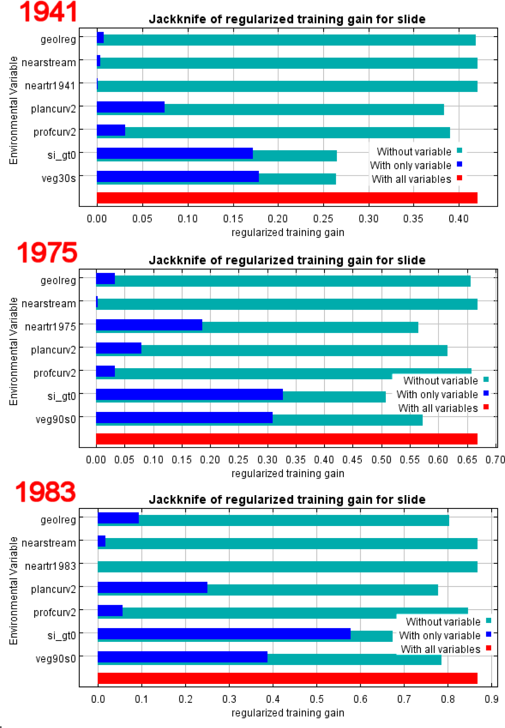
The landslide model for 1941 (AUC = 0.795) illustrates a preference for the areas of relatively moderate relief in the north-central part of the watershed, with vegetation and the SINMAP stability index contributing the most to the resulting model: 48% and 35%, respectively. Patterns of landslides reflect agricultural and grazing conditions prevalent until later residential development in the 1950’s. Many landslides occurred in scrubland areas on the steep eastern and southern hillslopes, though the north-central grassland shared a propensity for landslides, where grazing on hillslopes is a likely factor. Replacing the stability index with slope, however, produced identical results (AUC = 0.796), with slope contributing 59% of the model), suggesting no real improvement over stability index in the MaxEnt model. Stability index alone produced MaxEnt AUC of 0.652, while slope alone yielded an AUC of 0.687.
Similarly, in 1975, little difference results from choosing slope over SI, either alone (AUC for SI alone is 0.717, for slope alone is 0.719), or in combination with other factors (0.822 for the hybrid model with SI, 0.814 for a purely statistical model with slope). By 1975, the north-central area had experienced suburban development, with some landslide areas in the north central area landscaped and stabilized for housing. The greatest numbers of landslides occurred instead on steeper grassland and scrubland hillslopes to the east and south. Using landslide scars from 1983 as test data scored low in AUC, suggesting that the 1975 model reflects contrasting conditions in that year as compared with the later year. One likely factor is the prominence of suburban development and major expansion of trails, including off-road motorcycle trails [50], on hillslopes leading up to 1975, and this is shown by the 22.5% contribution of a 50-m trail buffer for the hybrid model and the 16.8% contribution of this factor in the purely statistical model employing slope.
The model from 1983 however does appear to show stability index contributing more than slope, at least as a single factor: when used alone, SI creates an AUC of 0.785, with slope alone creating an AUC of 0.749. But there is no real difference between the overall hybrid model (AUC of 0.859) and the statistical model employing slope (AUC = 0.857). In 1983, plan curvature and vegetation are the next most important contributors. Interestingly, numerous scars occur on the scrublands that dominate undeveloped steep hillslopes; it is likely that scrubland root structures do not extend deep enough to prevent landslides that result from an intense rainfall event. Similarly, only in the 1983 model does surficial geology play a prominent role, when landslides were abundant on colluvium, likely initiated from pore pressure threshold exceedances during the 1982 ENSO year [51].
Based on the mean and spread of receiver operator curves, the model worked much better for 1983 slope failures. This may have resulted from better landslide data from that more recent year, aided by better preservation of landslide scars that could be observed during field visits in later years. Another explanation may be the conditions leading to failures that likely provide a contrast between 1975 and 1983: the significance of impervious runoff in 1975 is less evident in 1983 in a lesser contribution of trail proximity, when under the intense 1982 ENSO rainfall events plan curvature (concentrating flow) appears to have played a more widespread role, in contrast to the possibly less predictable effects of impervious runoff.
In conclusion, the potential benefit of the hybrid approach will certainly take additional testing, perhaps also in larger study areas where spatial variability in rainfall intensity may play a part. While apparent from this and other studies that a maximum entropy model provides the ability to incorporate many variables that cannot be incorporated in a physical model alone, the results are difficult to apply generally, which is of course the appeal of a physical model. Our results suggest that while a stability measure developed via a physical modeling approach can provide more information than slope alone, slope in combination with plan curvature (influencing the concentration of hydrologic flows) and vegetation (influencing patterns of root cohesion) can provide similar overall predictive power. The potential benefit of the hybrid approach may be to better identify the contributing factors for initiating landslides by including a potentially clearer picture of slope stability variation from the physical model output, and one that can be improved with more spatially detailed soil parameters, but may benefit from the additional contribution of environmental factors influencing root cohesion and hydrologic flows, in a maximum-entropy model.
Author Contributions
Conceptualization of the project was initiated by Jerry Davis and further developed in discussions between the two authors. SINMAP, MaxEnt, and ArcGIS analysis and figures were completed by Jerry Davis. Composition of the document was completed by both authors. Both authors have read and approved the final manuscript.
Conflicts of Interest
The authors declare no conflict of interest.
References
- Varnes, D.J. Slope movement types and processes. In Landslides: Analysis and Control; Schuster, R.L., Krizek, R.J., Eds.; Volume Special Report 176; National Academy of Science Transportation Research Board: Washington, DC, USA, 1978; pp. 11–33. [Google Scholar]
- Schumm, S.A. Geomorphic thresholds: The concept and its applications. Trans. Inst. Br. Geogr. 1979, 4, 485–515. [Google Scholar]
- Uchida, T.; Kosugi, K.; Mizuyama, T. Effects of pipeflow on hydrological process and its relation to landslide: A review of pipeflow studies in forested headwater catchments. Hydrol. Process. 2001, 15, 2151–2174. [Google Scholar]
- Montgomery, D.R. Road surface drainage, channel initiation, and slope instability. Water Resour. Res. 1994, 30, 1925–1932. [Google Scholar]
- Iverson, R.M.; George, D.L.; Allstadt, K.; Reid, M.E.; Collins, B.D.; Vallance, J.W.; Schilling, S.P.; Godt, J.W.; Cannon, C.M.; Magirl, C.S. Landslide mobility and hazards: Implications of the 2014 Oso disaster. Earth Planet. Sci. Lett. 2015, 412, 197–208. [Google Scholar]
- Leshchinsky, B.A.; Olsen, M.J.; Tanyu, B.F. Contour Connection Method for automated identification and classification of landslide deposits. Comput. Geosci. 2015, 74, 27–38. [Google Scholar]
- Butt, M.; Umar, M.; Qamar, R. Landslide dam and subsequent dam-break flood estimation using HEC-RAS model in Northern Pakistan. Nat. Hazards 2013, 65, 241–254. [Google Scholar]
- Wills, C.J.; McCrink, T.P. Comparing landslide inventories: The map depends on the method. Environ. Eng. Geosci. 2002, VIII, 279–293. [Google Scholar]
- Van Westen, C.J.; Castellanos, E.; Kuriakose, S.L. Spatial data for landslide susceptibility, hazard, and vulnerability assessment: An overview. Eng. Geol. 2008, 102, 112–131. [Google Scholar]
- Martha, T.R.; Kerle, N.; Jetten, V.; van Westen, C.J.; Kumar, K.V. Characterising spectral, spatial and morphometric properties of landslides for semi-automatic detection using object-oriented methods. Geomorphology 2010, 116, 24–36. [Google Scholar]
- Parker, O.; Blesius, L. Object-Based Segmentation of Multi-Temporal Quickbird Imagery for Landslide Detection. Proceedings of XII International Symposium on Environmental Geotechnology, Energy and Global Sustainable Development, Los Angeles, CA, USA, 27–29 June 2012; Menezes, G.B., Moo-Young, H.K., Khachikian, C., de Brito Galvao, T.C., Eds.; Environmental Geotechnology: Los Angeles, CA, USA, 2012; pp. 291–299. [Google Scholar]
- Cascini, L. Applicability of landslide susceptibility and hazard zoning at different scales. Eng. Geol. 2008, 102, 164–177. [Google Scholar]
- Blesius, L.; Weirich, F. Shallow Landslide susceptibility mapping using stereo air photos and thematic maps. Cartogr. Geogr. Inf. Sci. 2010, 37, 105–118. [Google Scholar]
- Kavzoglu, T.; Sahin, E.K.; Colkesen, I. Landslide susceptibility mapping using GIS-based multi-criteria decision analysis, support vector machines and logistic regression. Landslides 2014, 11, 425–439. [Google Scholar]
- Dhakal, A.; Amada, T.; Aniya, M. Landslide hazard mapping and the application of GIS in the Kulekhani Watershed, Nepal. Mt. Res. Dev. 1999, 19, 3–16. [Google Scholar]
- Tosi, M. Root tensile strength relationships and their slope stability implications of three shrub species in the Northern Apennines (Italy). Geomorphology 2007, 87, 268–283. [Google Scholar]
- Rice, R.M.; Foggin, G.T. Effect of high intensity storms on soil slippage on mountainous watersheds in southern California. Water Resour. Res. 1971, 7, 1485–1496. [Google Scholar]
- Blesius, L.; Weirich, F. The use of high-resolution satellite imagery for deriving geotechnical parameters applied to landslide susceptibility. Proceedings of the ISPRS Hannover Workshop 2009 on High-resolution Earth Imaging for Geospatial Information, Hannover, Germany, 2–5 June 2009; Heipke, C., Jacobsen, K., Müller, S., Sörgel, U., Eds.; International Society for Photogrammetry and Remote Sensing: Hannover, Germany, 2009. [Google Scholar]
- Band, L.E.; Hwang, T.; Hales, T.C.; Vose, J.; Ford, C. Ecosystem processes at the watershed scale: Mapping and modeling ecohydrological controls of landslides. Geomorphology 2012, 137, 159–167. [Google Scholar]
- Cervi, F.; Berti, M.; Borgatti, L.; Ronchetti, F.; Manenti, F.; Corsini, A. Comparing predictive capability of statistical and deterministic methods for landslide susceptibility mapping: A case study in the northern Apennines (Reggio Emilia Province, Italy). Landslides 2010, 7, 433–444. [Google Scholar]
- Althuwaynee, O.F.; Pradhan, B.; Park, H.-J.; Lee, J.H. A novel ensemble decision tree-based CHi-squared Automatic Interaction Detection (CHAID) and multivariate logistic regression models in landslide susceptibility mapping. Landslides 2014, 11, 1063–1078. [Google Scholar]
- Tien Bui, D.; Tuan, T.A.; Klempe, H.; Pradhan, B.; Revhaug, I. Spatial prediction models for shallow landslide hazards: A comparative assessment of the efficacy of support vector machines, artificial neural networks, kernel logistic regression, and logistic model tree. Landslides 2015. [Google Scholar] [CrossRef]
- Tien Bui, D.; Pradhan, B.; Lofman, O.; Revhaug, I.; Dick, O.B. Spatial prediction of landslide hazards in Hoa Binh province (Vietnam): A comparative assessment of the efficacy of evidential belief functions and fuzzy logic models. Catena 2012, 96, 28–40. [Google Scholar]
- Haigh, M.J. Dynamic systems approaches in landslide hazard risk. Z. Fuer Geomorphol. 1988, 67, 79–91. [Google Scholar]
- Phillips, S.; Anderson, R.; Schapire, R. Maximum entropy modeling of species geographic distributions. Ecol. Model. 2006, 190, 231–259. [Google Scholar]
- Convertino, M.; Troccoli, A.; Catani, F. Detecting fingerprints of landslide drivers: A MaxEnt model. J. Geophys. Res. Earth Surf. 2013, 118, 1367–1386. [Google Scholar]
- Brabb, E.E.; Pampeyan, E.H.; Bonilla, M.G. Landslide susceptibility in San Mateo County California scale 1:62500. In Miscellaneous Field Studies Map MF-360; US Geological Survey: Reston, VA, USA, 1972. [Google Scholar]
- Kashiwagi, J.H.; Hokholt, L.A. Soil Survey of San Mateo County, Eastern part, and San Francisco County, California; U.S. Department of Agriculture, Soil Conservation Service: Washington, DC, USA, 1991. [Google Scholar]
- Soil Survey Staff. Soil Taxonomy, A Basic System of Soil Classification for Making and Interpreting Soil Surveys, 2nd ed; US Department of Agriculture, Natural Resources Conservation Service: Washington DC, USA, 1999; Volume Agriculture Handbook #436; p. 869. [Google Scholar]
- Pampeyan, E.H. Geologic Map of the Montara Mountain and San Mateo 7–1/2′ Quadrangles, San Mateo County, California, Scale 1:24,000; US Geological Survey: Reston, VA, USA, 1994. [Google Scholar]
- Brabb, E.E.; Pampeyen, E.H. Preliminary map of landslide deposits in San Mateo County, California, scale 1:62,500. In Miscellaneous Field Studies Map MF-344; U.S. Geological Survey: Reston, VA, USA, 1972. [Google Scholar]
- Sims, S. Hillslope sediment source assessment of San Pedro Creek Watershed, California. Master’s Thesis, The San Francisco State University, San Francisco, CA, USA, 2004. [Google Scholar]
- United States Army Corps of Engineers, San Francisco District. San Pedro Creek Section 205 Flood Control Study; Engineers, U.S. Army Corps of Engineers: San Francisco, 1998. [Google Scholar]
- Pack, R.; Tarboton, D.; Goodwin, C.; Prasad, A. A Stability Index Approach to Terrain Stability Hazard Mapping 2005, User’s Manual; CEE Faculty Publications: Logan, UT, USA, 2005. Avaliable online: http://hydrology.usu.edu/sinmap2/ accessed on 8 May 2013.
- Dyke, J.; Kleidon, A. The maximum entropy production principle: Its theoretical foundations and applications to the earth system. Entropy 2010, 12, 613–630. [Google Scholar]
- Phillips, J.D. Divergence, convergence, and self-organization in landscapes. Ann. Assoc. Am. Geogr. 1999, 89, 466–488. [Google Scholar]
- Elith, J.; Phillips, S.; Hastie, T.; Dudík, M.; Chee, Y.; Yates, C. A statistical explanation of MaxEnt for ecologists. Divers. Distrib. 2011, 17, 43–57. [Google Scholar]
- Ruddell, B.L.; Brunsell, N.A.; Stoy, P. Applying information theory in the geosciences to quantify process uncertainty, feedback, scale. Eos Trans. Am. Geophys. Union 2013, 94, 56. [Google Scholar]
- Felicísimo, Á.; Cuartero, A.; Remondo, J.; Quirós, E. Mapping landslide susceptibility with logistic regression, multiple adaptive regression splines, classification and regression trees, and maximum entropy methods: A comparative study. Landslides 2013, 10, 175–189. [Google Scholar]
- Phillips, S.; Dudík, M. Modeling of species distributions with Maxent: New extensions and a comprehensive evaluation. Ecography 2008, 31, 161–175. [Google Scholar]
- Ghestem, M.; Sidle, R.; Stokes, A. The influence of plant root systems on subsurface flow: Implications for slope stability. BioScience 2011, 61, 869–879. [Google Scholar]
- Reneau, S.L.; Dietrich, W.E.; Donahue, D.J.; Jull, A.J.T.; Rubin, M. Late Quaternary history of colluvial deposition and erosion in hollows, central California Coast Ranges. Geol. Soc. Am. Bull. 1990, 102, 969–982. [Google Scholar]
- Rib, H.T.; Liang, T. Landslides: Analysis and control. In Recognition and Identification; Schuster, R.L., Krizek, R.J., Eds.; Volume Special Report 176; National Academy of Sciences: Washington, DC, USA, 1978; pp. 34–80. [Google Scholar]
- Collins, L.; Amato, P.; Morton, D. San Pedro Creek geomorphic analysis. In San Pedro Creek Watershed Assessment and Enhancement Plan; San Pedro Creek Watershed Coalition: Pacifica, CA, USA, 2001; pp. 631–646. [Google Scholar]
- Howard, T.R.; Baldwin, J.E.; Donley, H.F. Landslides in Pacifica California caused by the storm. In Landslides Floods and Marine Effects of the Storm of January 3–5, 1982 in the San Francisco Bay Region California; Volume US Geological Survey Professional Paper 1434; US Geological Survey: Reston, VA, USA, 1988; pp. 3–5. [Google Scholar]
- Cannon, S.H.; Ellen, S.D. Rainfall that resulted in abundant debris-flow activity during the storm. In Landslides, Floods, and Marine Effects of the Storm of January 3–5 1982 in the San Francisco Bay Region, California; Volume US Geological Survey Professional Paper 1434; U.S. Geological Survey: Reston, VA, USA, 1988; pp. 3–5. [Google Scholar]
- Davis, J.D.; Sims, S.M. Physical and maximum entropy models applied to inventories of hillslope sediment sources. J. Soils Sediments 2013, 13, 1784–1801. [Google Scholar]
- Wieslander, A.E. A vegetation type map of California. Madroño 1935, 3, 140–144. [Google Scholar]
- Davis, J.D.; Matuk, V.; Wilkinson, N.L.; Chan, C. San Pedro Creek Watershed Assessment and Enhancement Plan; San Pedro Creek Watershed Coalition: Pacifica, CA, USA, 2002. [Google Scholar]
- Davis, J.D.; Davis, A.W.; Harvey, B.J. Pedro Point Headlands 1941 to 2010: A Preliminary Study Using Historical Remote Sensing and Dendrochronology; Pacifica Land Trust: Pacifica, CA, USA, 2010. [Google Scholar]
- Wieczorek, G.F.; Harp, E.L.; Mark, R.K.; Bhattacharyya, A.K. Debris flows and other landslides in San Contra Costa, Alameda, Napa, Solano, Sonoma, Lake, and Yolo Counties, and other factors influencing debris-flow distribution. In Landslides, Floods, and Marine Effects of the Storm of January 3–5, 1982 in the San Francisco Bay Region, California; Volume US Geological Survey Professional Paper 1434; U.S. Geological Survey: Reston, VA, USA, 1988; pp. 3–5. [Google Scholar]
Figure 1.
Surficial geology of San Pedro Creek watershed, after Pampeyan [30].
Figure 1.
Surficial geology of San Pedro Creek watershed, after Pampeyan [30].

Figure 2.
Streams, roads and trails in San Pedro Creek watershed.

Figure 3.
Major vegetation types in undeveloped areas, San Pedro Creek watershed, based upon field mapping in 2002.
Figure 3.
Major vegetation types in undeveloped areas, San Pedro Creek watershed, based upon field mapping in 2002.

Figure 4.
Shallow landslides associated with impervious runoff in San Pedro Creek watershed. At left is the crest of a failure that occurred below Higgins Road in 2003; at right are older scars from the 1970’s below a dirt road above Picardo Ranch. (Photographs by Jerry Davis)
Figure 4.
Shallow landslides associated with impervious runoff in San Pedro Creek watershed. At left is the crest of a failure that occurred below Higgins Road in 2003; at right are older scars from the 1970’s below a dirt road above Picardo Ranch. (Photographs by Jerry Davis)

Figure 5.
Hybrid model combining a physical infinite-slope model extended spatially via soil thickness and transmissivity using downslope accumulated flows (SINMAP) with a maximum entropy (MaxEnt) model. SINMAP runs in ArcGIS, and ArcGIS geoprocessing tools are used to generate slope, plan curvature, stream distance and trail/road distance. If slope is used instead of stability index, this produces a purely statistical maximum-entropy model.

Figure 6.
Slope-Area Plot generated by SINMAP, with inventory landslides from all years plotted with boundary curves of stability index and saturation.
Figure 6.
Slope-Area Plot generated by SINMAP, with inventory landslides from all years plotted with boundary curves of stability index and saturation.

Figure 7.
Locations where landslides were first visible in 1941, 1975 and 1983, plotted on SINMAP Stability Index.
Figure 7.
Locations where landslides were first visible in 1941, 1975 and 1983, plotted on SINMAP Stability Index.

Figure 8.
Receiver operator curves (ROC) generated by MaxEnt for 1941, 1975, and 1983 landslides, from 10-fold replicate models. Receiving operator curves are shown as the total range of replicate curves, with the mean curve in red.
Figure 8.
Receiver operator curves (ROC) generated by MaxEnt for 1941, 1975, and 1983 landslides, from 10-fold replicate models. Receiving operator curves are shown as the total range of replicate curves, with the mean curve in red.

Figure 9.
Variable contribution jackknife plots generated by MaxEnt for 1941, 1975, and 1983 landslides, from 10-fold replicate models. Jackknife plots provide the variable contributions from geology (geolreg), proximity to streams (nearstream), proximity to trails (neartr_), plan curvature (plancurv2), profile curvature (profcurv2), stability index (si_gt0), and vegetation (veg_).

Figure 10.
Maps generated by MaxEnt for 1941, 1975, and 1983 landslides, from 10-fold replicate models.
Figure 10.
Maps generated by MaxEnt for 1941, 1975, and 1983 landslides, from 10-fold replicate models.


Table 1.
SINMAP inputs for transmissivity (T), recharge (R), cohesion (C), friction (φ), and density (ρ). Soil data from Natural Resources Conservation Service SSURGO data, modified with colluvium depths from [30].
| Parent material | Soil depth (m) | Hydraulic conductivity (m h−1) | T (m2 h−1) | R (m h−1) | T/R (m) | C | Φ (°) | Ρ (kg m−3) |
|---|---|---|---|---|---|---|---|---|
| granitic | 1 | 0.10 | 0.1 | 0.0002–0.0042 | 24–500 | 0–0.25 | 30–45 | 2000 |
| colluvium | 3 | 0.03 | 0.1 | 0.0002–0.0042 | 24–500 | 0–0.25 | 30–45 | 2000 |
| Imagery Year | 1941 | 1955 | 1975 | 1983 | 1997 |
|---|---|---|---|---|---|
| n scars | 154 | 39 | 142 | 253 | 10 |
| n SI < 1.0 | 91 | 24 | 91 | 197 | 6 |
| % | 59% | 62% | 64% | 78% | 60% |
Table 3.
Maxent results by year of shallow landslide scars from aerial photography, including overall and 10-fold replicate models. Variables were chosen based upon their contribution to one or more models, and correlated variables (SI and slope) were not used together. Variable contributions are given as percent contribution (%) and permutation importance (PI). Models are evaluated as AUC for a threshold-independent assessment; for a threshold-dependent evaluation, arithmetic means of the 10 p values use the maximum test sensitivity + specificity threshold from MaxEnt [40]. Lambdas for categorical variables are for unreplicated models using all data for training.
| 1941 | 1975 | 1983 | |||||
|---|---|---|---|---|---|---|---|
| using: | SI | slope | SI | slope | SI | slope | |
| n | 132 | 154 | 132 | 141 | 226 | 252 | |
| AUC (using all data) | 0.795 | 0.796 | 0.822 | 0.814 | 0.859 | 0.857 | |
| AUC subsequent-year test data | 0.778 | 0.795 | 0.749 | 0.742 | 0.853 | 0.842 | |
| subsequent test year | 1955 | 1983 | 1997 | ||||
| n slides in test year | 31 | 39 | 226 | 253 | 9 | 10 | |
| 10-fold replicates: | |||||||
| AUC with 10-fold replicates | 0.728 | 0.743 | 0.782 | 0.772 | 0.839 | 0.836 | |
| AUC standard deviation | 0.044 | 0.041 | 0.058 | 0.040 | 0.026 | 0.024 | |
| p: maximum test sensitivity + specificity | 0.004 | 0.041 | 0.001 | 0.000 | 0.000 | 0.000 | |
| SINMAP stability index | %C | 48.1 | 35.3 | 48 | |||
| PI | 50.2 | 49.7 | 57.4 | ||||
| Slope (°) | %C | 59.1 | 41 | 37.5 | |||
| PI | 59.3 | 49.2 | 46.4 | ||||
| Plan curvature | %C | 9.6 | 13.4 | 6.4 | 7.4 | 15.3 | 19.6 |
| PI | 9.4 | 15 | 3.9 | 6.6 | 13.9 | 18.8 | |
| Profile curvature | %C | 6.7 | 2.3 | 1.5 | 1.1 | 2.2 | 1.7 |
| PI | 10.1 | 4.8 | 4.2 | 3.1 | 5 | 2.7 | |
| 50-m trail buffer | %C | 0 | 0.3 | 22.5 | 16.8 | 0.1 | 0 |
| PI | 0 | 0.2 | 14.9 | 16.4 | 0.1 | 0 | |
| Vegetation | %C | 35 | 23.7 | 32.2 | 33.2 | 24.6 | 27 |
| PI | 29.9 | 20 | 24.9 | 23.6 | 15.5 | 20.3 | |
| 0. Farmed (1941), Developed (1975 & 1983) λ | 0.0 | 0.00 | −1.93 | −2.14 | −0.02 | −0.42 | |
| 1. Grassland λ | 1.76 | 1.17 | 1.06 | 1.25 | |||
| 2. Scrublands λ | 0.54 | 1.43 | 1.39 | ||||
| 3. Forest λ | −0.01 | −0.56 | −0.34 | ||||
| Geology | %C | 0.5 | 1.1 | 2.1 | 0.6 | 9.8 | 13.4 |
| PI | 0.1 | 0.7 | 2.2 | 1.2 | 7.9 | 11.4 | |
| 1. Granitic λ | −0.22 | −0.40 | 0.0 | 0.0 | −1.10 | −1.03 | |
| 2. Sandstone λ | 0.03 | 0.15 | |||||
| 3. Colluvium λ | 0.03 | −0.33 | −0.02 | 0.54 | 0.58 | ||
© 2015 by the authors; licensee MDPI, Basel, Switzerland This article is an open access article distributed under the terms and conditions of the Creative Commons Attribution license (http://creativecommons.org/licenses/by/4.0/).
Share and Cite
MDPI and ACS Style
Davis, J.; Blesius, L. A Hybrid Physical and Maximum-Entropy Landslide Susceptibility Model. Entropy 2015, 17, 4271-4292. https://doi.org/10.3390/e17064271
AMA Style
Davis J, Blesius L. A Hybrid Physical and Maximum-Entropy Landslide Susceptibility Model. Entropy. 2015; 17(6):4271-4292. https://doi.org/10.3390/e17064271
Chicago/Turabian StyleDavis, Jerry, and Leonhard Blesius. 2015. "A Hybrid Physical and Maximum-Entropy Landslide Susceptibility Model" Entropy 17, no. 6: 4271-4292. https://doi.org/10.3390/e17064271