Analysis of the Keller–Segel Model with a Fractional Derivative without Singular Kernel

Abstract

Using some investigations based on information theory, the model proposed by Keller and Segel was extended to the concept of fractional derivative using the derivative with fractional order without singular kernel recently proposed by Caputo and Fabrizio. We present in detail the existence of the coupled-solutions using the fixed-point theorem. A detailed analysis of the uniqueness of the coupled-solutions is also presented. Using an iterative approach, we derive special coupled-solutions of the modified system and we present some numerical simulations to see the effect of the fractional order.

1. Introduction

The mathematical exemplification of the environments and parameters affecting the diffusion and management of information is referred as to information theory. Information theory is a branch of applied mathematics, electrical engineering and computer science involving the quantification of information. In applied mathematics, to model real world problem, one needs to observe the physical behavior of the problem and then convert it into mathematical formulas. The concept of information theory is therefore needed to accurately represent the physical problem in mathematical formula, and quantify problem uncertainties via entropy in order to have better prediction. Other important applications of information theory can be found in [1–5]. The field of fractional order derivatives has attracted the attention of many researchers in all branches of sciences and engineering. In recent years, many field of sciences and technology have used fractional order derivatives to model many real world problems in their respective fields, as it has been revealed that these fractional order derivatives are very efficient in describing such problems [6–12]. It is no wonder therefore why many researchers in the field of fractional calculus have devoted their attention to proposing new fractional order derivatives [13–19].

These derivative definitions range from the well-known Riemann–Liouville derivative to the newly proposed one known as the Caputo–Fabrizio derivative. It is very important to note that most of these definitions are based on the convolution. The definitions proposed by Riemann–Liouville and the first Caputo version has the weakness that their kernel had singularity. Since the kernel is used to describe the memory effect of the system, it is clear that with this weakness, these two derivatives cannot accurately describe the full effect of the memory. To further enhance the full description of memory, Caputo and Fabrizio have recently introduced a new fractional order derivative without a singular kernel [16,20,21]. In their paper, they demonstrated that the interest in the new derivative is because of the requirement of exploiting the performance of the conventional viscoelastic materials, thermal media, electromagnetic systems and others. However, they pointed out the fact that the commonly used fractional derivatives were designed to deal with mechanical phenomena, connected to plasticity, fatigue, damage and also electromagnetic hysteresis [20]. Therefore the new derivative can be used outside the scope of the described field. More importantly, their proposed derivative is able to portray material heterogeneities and structures at different scales [20]. The aim of this paper is to check the possibility of applying this new derivative to other branches of sciences, in particular epidemiology. In this work, we will modify the model proposed by Keller and Segel [22–26] by replacing the ordinary time derivative with the Caputo–Fabrizio fractional order derivative. In the knowledge that the new derivative is not popular, we will first present some useful information about this derivative to inform those readers that are not aware of it.

2. The Caputo and Fabrizio Fractional Order Derivative

The main problem faced with the first definition of fractional order derivative is the singularity at the end point of the interval. To avoid the singularity, Caputo and Fabrizio recently proposed a fractional order derivative without any singularity worries. The definition is based on the convolution of a first order derivative and the exponential function, given in the following definition:

Definition 1. Let$f\in H^1\left(a,b\right),b>a,\alpha \in [0,1]$ then, the new Caputo derivative of a fractional derivative is defined as:

$$D_t^{\alpha }\left(f\left(t\right)\right)=\frac{M(\alpha )}{1-\alpha }\underset{a}{\overset{t}{{\displaystyle \int }}}f\prime (x)exp\left[-\alpha \frac{t-x}{1-\alpha }\right]dx$$

(1)

where$M(\alpha )$ is a normalization function such that$M\left(0\right)=M\left(1\right)=1$ [20]. However, if the function does not belong to$H^1\left(a,b\right)$ then, the derivative can be reformulated as:

$$D_t^{\alpha }\left(f\left(t\right)\right)=\frac{\alpha M(\alpha )}{1-\alpha }\underset{a}{\overset{t}{{\displaystyle \int }}}\left(f\left(t\right)-f(x)\right)exp\left[-\alpha \frac{t-x}{1-\alpha }\right]dx$$

Remark 1. The instigators observed that, if$\sigma =\frac{1-\alpha }{\alpha }\in \left[0,\infty \right),\alpha =\frac{1}{1+\sigma }\in [0,1]$, then Equation (2) assumes the form:

$$D_t^{\alpha }\left(f\left(t\right)\right)=\frac{N(\sigma )}{\sigma }\underset{a}{\overset{t}{{\displaystyle \int }}}f\prime \left(x\right)exp\left[-\frac{t-x}{\sigma }\right]dx,N\left(0\right)=N\left(\infty \right)=1$$

(2)

In addition:

$$\underset{\sigma \to 0}{\lim }\frac{1}{\sigma }exp\left[-\frac{t-x}{\sigma }\right]=\delta \left(x-t\right)$$

(3)

At this instant subsequent to the preface of the novel derivative, the connected anti-derivative, the associate integral, turns out to be imperative [23,24].

Definition 2. Let$0<\alpha <1.$ The fractional integral of order$\alpha$ of a function$f$ is defined as:

$$I_{\alpha }^t(f(t))=\frac{2(1-\alpha )}{(2-\alpha )M(\alpha )}f(t)+\frac{2\alpha }{(2-\alpha )M(\alpha )}\underset{t}{\overset{0}{{\displaystyle \int }}}f(s)ds,t\ge 0$$

(4)

Remark 2. Note that, according to the above definition, the fractional integral of Caputo type of function of order$0<\alpha <1$ is an average between function f and its integral of order one. This therefore imposes the condition [21]:

$$\frac{2\left(1-\alpha \right)}{\left(2-\alpha \right)M\left(\alpha \right)}+\frac{2\alpha }{\left(2-\alpha \right)M\left(\alpha \right)}=1$$

(5)

The above expression yields an explicit formula:

$$M\left(\alpha \right)=\frac{2}{2-\alpha },0\le \alpha \le 1$$

Because of the above, Nieto and Losada [21] proposed that the new Caputo derivative of order $0<\alpha <1$ can be reformulated as:

$$D_t^{\alpha }\left(f\left(t\right)\right)=\frac{1}{1-\alpha }\underset{a}{\overset{t}{{\displaystyle \int }}}f\prime (x)exp\left[-\alpha \frac{t-x}{1-\alpha }\right]dx$$

(6)

Theorem 1. For the new Caputo fractional order derivative, if the function$f(t)$ is such that:

$$f^{\left(s\right)}\left(a\right)=0,s=1,2,\dots n$$

then, we have:

$$D_t^{\alpha }\left(D_t^n(f(t))\right)=D_t^n\left(D_t^{\alpha }(f(t))\right)$$

The proof this can be found in [20,21].

3. Chemotaxis Model Proposed by Keller and Segel

Keller and Segel proposed the dynamic model of the aggregation process of cellular slime mold by chemical attraction in 1970. The simplified model in one dimension of the model is given by:

$$\{\begin{array}{c}\frac{\partial u(x,t)}{\partial t}=a\frac{{\partial }^{2}u(x,t)}{\partial x^2}-\frac{\partial }{\partial x}\left(u(x,t)\frac{\partial \phi (\rho (x,t))}{\partial x}\right)\\ \frac{\partial \rho (x,t)}{\partial t}=b\frac{{\partial }^2\rho (x,t)}{\partial x^2}+cu\left(x,t\right)-d\rho (x,t)\end{array}$$

(7)

The associated initial conditions to the above system are given as:

$$u\left(x,0\right)=u_0\left(x\right),\rho \left(x,0\right)={\rho }_0\left(x\right),x\in I=(\alpha ,\beta )$$

$a,b,c,$ and $d$ are positive constants. The coupled solutions $\rho (x,t)$ and $u(x,t)$ represent the concentration of a chemical substance and concentration of amoebae, respectively. The sensibility of the chemicals and attraction of terms are indicated by the chemotactic expression:

$$\frac{\partial }{\partial x}\left(u(x,t)\frac{\partial \phi (\rho \frac{\partial }{\partial x}\left(u(x,t)\frac{\partial \phi (\rho (x,t))}{\partial x}\right)(x,t))}{\partial x}\right)$$

(8)

The term $\phi (\rho (x,t))$ represents the sensitivity function, and is a smooth function of $\rho \in (0,\infty )$ which described a cell’s perception and response to chemical stimulus. However, the above model is not able to describe the effect of memory and also the movement of the bacteria within different layers of the medium via which the global movement is taking place. Therefore in order to include these two effects into the mathematical formulation, we modified the system by replacing the ordinary time derivative to the newly proposed fractional order derivative as follows:

$$\{\begin{array}{c}{}_0{}^{CF}D{}_t^{\alpha }u(x,t)=a\frac{{\partial }^{2}u(x,t)}{\partial x^2}-\frac{\partial }{\partial x}\left(u(x,t)\frac{\partial \phi (\rho (x,t))}{\partial x}\right)\\ {}_0{}^{CF}D{}_t^{\alpha }\rho (x,t)=b\frac{{\partial }^2\rho (x,t)}{\partial x^2}+cu\left(x,t\right)-d\rho (x,t)\end{array}$$

(9)

To be more precise, we chose the sensitivity function to be:

$$\phi \left(\rho \left(x,t\right)\right)=\frac{\rho (x,t)}{\rho \left(x,t\right)+1},\rho \left(x,t\right),\frac{{\rho }^2(x,t)}{{\rho }^2\left(x,t\right)+1},log\left(\rho \left(x,t\right)\right)$$

(10)

The initial conditions are the same as in Equation (8).

3.1. Existence of Coupled Solutions

In this section, using the fixed-point theorem, we present the existence of the coupled-solution. We first transform Equation (9) to an integral equation as follows:

$$\{\begin{array}{c}u\left(x,t\right)-u\left(x,0\right)={}_0{}^{CF}I{}_t^{\alpha }\left\{a\frac{{\partial }^{2}u(x,t)}{\partial x^2}-\frac{\partial }{\partial x}\left(u(x,t)\frac{\partial \phi (\rho (x,t))}{\partial x}\right)\right\}\\ \rho \left(x,t\right)-\rho \left(x,0\right)={}_0{}^{CF}I{}_t^{\alpha }\left\{b\frac{{\partial }^2\rho (x,t)}{\partial x^2}+cu\left(x,t\right)-d\rho (x,t)\right\}\end{array}$$

Using the notation proposed by Nieto, we obtain:

$$\{\begin{array}{c}u\left(x,t\right)-u\left(x,0\right)=\frac{2\left(1-\alpha \right)}{\left(2-\alpha \right)M\left(\alpha \right)}\left\{a\frac{{\partial }^{2}u\left(x,t\right)}{\partial x^2}-\frac{\partial }{\partial x}\left(u\left(x,t\right)\frac{\partial \phi \left(\rho \left(x,t\right)\right)}{\partial x}\right)\right\}+\\ \frac{2\alpha }{\left(2-\alpha \right)M\left(\alpha \right)}\underset{0}{\overset{t}{{\displaystyle \int }}}\left\{a\frac{{\partial }^{2}u\left(x,y\right)}{\partial x^2}-\frac{\partial }{\partial x}\left(u\left(x,y\right)\frac{\partial \phi \left(\rho \left(x,y\right)\right)}{\partial x}\right)\right\}dy\\ \rho \left(x,t\right)-\rho \left(x,0\right)=\frac{2\left(1-\alpha \right)}{\left(2-\alpha \right)M\left(\alpha \right)}\left\{b\frac{{\partial }^2\rho \left(x,t\right)}{\partial x^2}+cu\left(x,t\right)-d\rho \left(x,t\right)\right\}+\\ \frac{2\alpha }{\left(2-\alpha \right)M\left(\alpha \right)}\underset{0}{\overset{t}{{\displaystyle \int }}}\left\{b\frac{{\partial }^2\rho (x,y)}{\partial x^2}+cu\left(x,y\right)-d\rho (x,y)\right\}dy\end{array}$$

(11)

For simplicity, we define the following kernels:

$$\begin{array}{c}{K}_1\left(x,t,u\right)=a\frac{{\partial }^{2}u\left(x,y\right)}{\partial x^2}-\frac{\partial }{\partial x}\left(u\left(x,y\right)\frac{\partial \phi \left(\rho \left(x,y\right)\right)}{\partial x}\right)\\ K_2\left(x,t,\rho \right)=b\frac{{\partial }^2\rho (x,y)}{\partial x^2}+cu\left(x,y\right)-d\rho (x,y)\end{array}$$

(12)

Theorem 2.$K_1$ and$K_2$ satisfy the Lipschiz condition and contraction if the following inequality holds:

$$0<a{\delta }_1^2+{\delta }_2\Vert \frac{\partial \phi \left(\rho \left(x,t\right)\right)}{\partial x}\Vert \le 1$$

Proof. We shall start with $K_1$. Let $u$and $v$ be two functions, then we evaluate the following:

$$\Vert K_1\left(x,t,u\right)-K_1\left(x,t,v\right)\Vert =\Vert a\frac{{\partial }^2\left\{u\left(x,t\right)-v(x,t)\right\}}{\partial x^2}-\frac{\partial }{\partial x}\left(\left\{u\left(x,t\right)-v(x,t)\right\}\frac{\partial \phi \left(\rho \left(x,t\right)\right)}{\partial x}\right)\Vert$$

(13)

Using the triangular inequality, we transform the above Equation (13) to:

$$\Vert K_1(x,t,u)-K_1(x,t,v)\Vert \le \Vert a\frac{{\partial }^2\{u(x,t)-v(x,t)\}}{\partial x^2}\Vert +\Vert -\frac{\partial }{\partial x}(\{u(x,t)-v(x,t)\}\frac{\partial \phi (\rho (x,t))}{\partial x})\Vert$$

Knowing that the operator derivative satisfies the Lipchitz condition, we can then find two positive parameters ${\delta }_1$ and ${\delta }_2$ such that:

$$\begin{array}{c}a\Vert \frac{{\partial }^2\{u(x,t)-v(x,t)\}}{\partial x^2}\Vert \le a{\delta }_1^2\Vert u(x,t)-v(x,t)\Vert \\ \Vert -\frac{\partial }{\partial x}(\{u(x,t)-v(x,t)\}\frac{\partial \phi (\rho (x,t))}{\partial x})\Vert \le {\delta }_2\Vert \frac{\partial \phi (\rho (x,t))}{\partial x}\Vert \Vert u(x,t)-v(x,t)\Vert \end{array}$$

(14)

Replacing Equation (14) into Equation (12), we obtain:

$$\Vert K_1(x,t,u)-K_1(x,t,v)\Vert \le \{a{\delta }_1^2+{\delta }_2\Vert \frac{\partial \phi (\rho (x,t))}{\partial x}\Vert \}\Vert u(x,t)-v(x,t)\Vert$$

(15)

Taking:

$$H=\left\{a{\delta }_1^2+{\delta }_2\Vert \frac{\partial \phi \left(\rho \left(x,t\right)\right)}{\partial x}\Vert \right\}$$

then:

$$\Vert K_1\left(x,t,u\right)-K_1\left(x,t,v\right)\Vert \le H\Vert u\left(x,t\right)-v(x,t)\Vert$$

Therefore $K_1$ satisfies the Lipschiz conditions and if in addition:

$$0<a{\delta }_1^2+{\delta }_2\Vert \frac{\partial \phi \left(\rho \left(x,t\right)\right)}{\partial x}\Vert \le 1$$

then it is also a contraction.

With the second case we have that, the kernel is linear then it satisfies the Lipchitz condition as follows:

$$\Vert K_2(x,t,\rho )-K_2(x,t,{\rho }_1)\Vert \le \{b{\theta }_1^2+c\}\Vert \rho (x,t)-{\rho }_1(x,t)\Vert$$

Considering these kernels, Equation (11) is reduced to:

$$\{\begin{array}{c}u\left(x,t\right)=\frac{2\left(1-\alpha \right)}{\left(2-\alpha \right)M\left(\alpha \right)}{K}_1\left(x,t,u\right)+u\left(x,0\right)+\frac{2\alpha }{\left(2-\alpha \right)M\left(\alpha \right)}\underset{0}{\overset{t}{{\displaystyle \int }}}\left\{K_1\left(x,t,u\right)\right\}dy\\ \rho \left(x,t\right)=\frac{2\left(1-\alpha \right)}{\left(2-\alpha \right)M\left(\alpha \right)}{K}_2\left(x,t,\rho \right)+\rho \left(x,0\right)+\frac{2\alpha }{\left(2-\alpha \right)M\left(\alpha \right)}\underset{0}{\overset{t}{{\displaystyle \int }}}{K}_2\left(x,t,\rho \right)dy\end{array}$$

(16)

We consider the following recursive formula:

$$\{\begin{array}{c}{u}_n\left(x,t\right)=\frac{2\left(1-\alpha \right)}{\left(2-\alpha \right)M\left(\alpha \right)}{K}_1\left(x,t,u_{n-1}\right)+\frac{2\alpha }{\left(2-\alpha \right)M\left(\alpha \right)}\underset{0}{\overset{t}{{\displaystyle \int }}}\left\{K_1\left(x,t,u_{n-1}\right)\right\}dy\\ {\rho }_n\left(x,t\right)=\frac{2\left(1-\alpha \right)}{\left(2-\alpha \right)M\left(\alpha \right)}{K}_2\left(x,t,{\rho }_{n-1}\right)+\frac{2\alpha }{\left(2-\alpha \right)M\left(\alpha \right)}\underset{0}{\overset{t}{{\displaystyle \int }}}{K}_2\left(x,t,{\rho }_{n-1}\right)dy\end{array}$$

(17)

With initial component

$$\{\begin{array}{l}{u}_0\left(x,t\right)=u(x,0)\\ {\rho }_0\left(x,t\right)=\rho \left(x,0\right)\end{array}$$

The difference between the consecutive terms is given as:

$$\begin{array}{l}{U}_n(x,t)=u_n(x,t)-u_{n-1}(x,t)=\frac{2(1-\alpha )}{(2-\alpha )M(\alpha )}{K}_1(x,t,u_{n-1})-\frac{2(1-\alpha )}{(2-\alpha )M(\alpha )}{K}_1(x,t,u_{n-2})+\frac{2\alpha }{(2-\alpha )M(\alpha )}\underset{0}{\overset{t}{{\displaystyle \int }}}\left\{K_1(x,t,u_{n-1})-K_1(x,t,u_{n-2})\right\}dy\\ V_n(x,t)={\rho }_n(x,t)-{\rho }_{n-1}(x,t)=\frac{2(1-\alpha )}{(2-\alpha )M(\alpha )}{K}_2(x,t,{\rho }_{n-1}-{\rho }_{n-1})+\frac{2\alpha }{(2-\alpha )M(\alpha )}\underset{0}{\overset{t}{{\displaystyle \int }}}{K}_2(x,t,{\rho }_{n-1}-{\rho }_{n-1})dy\end{array}$$

(18)

It worth noting that:

$$\{\begin{array}{l}{u}_n\left(x,t\right)={\displaystyle \sum }_{i=0}^n{U}_i(x,t)\\ {\rho }_n\left(x,t\right)={\displaystyle \sum }_{i=0}^n{V}_i(x,t)\end{array}$$

Step-by-step we evaluate:

$$\Vert U_n(x,t)\Vert =\Vert u_n(x,t)-u_{n-1}(x,t)\Vert =\Vert \frac{2(1-\alpha )}{(2-\alpha )M(\alpha )}{K}_1(x,t,u_{n-1})-\frac{2(1-\alpha )}{(2-\alpha )M(\alpha )}{K}_1(x,t,u_{n-2})+\frac{2\alpha }{(2-\alpha )M(\alpha )}\underset{t}{\overset{0}{{\displaystyle \int }}}\{K_1(x,t,u_{n-1})-K_1(x,t,u_{n-2})\}dy\Vert$$

Using the triangular inequality; the above equation becomes:

$$\Vert u_n(x,t)-u_{n-1}(x,t)\Vert \le \frac{2(1-\alpha )}{(2-\alpha )M(\alpha )}\Vert K_1(x,t,u_{n-1})-K_1(x,t,u_{n-2})\Vert +\frac{2\alpha }{(2-\alpha )M(\alpha )}\Vert \underset{0}{\overset{t}{{\displaystyle \int }}}\{K_1(x,t,u_{n-1})-K_1(x,t,u_{n-2})\}dy\Vert$$

(19)

Since the kernel satisfies the Lipchitz condition, we obtain:

$$\Vert u_n(x,t)-u_{n-1}(x,t)\Vert \le \frac{2(1-\alpha )}{(2-\alpha )M(\alpha )}H\Vert u_{n-1}-u_{n-2}\Vert +\frac{2\alpha }{(2-\alpha )M(\alpha )}K\underset{t}{\overset{0}{{\displaystyle \int }}}\Vert u_{n-1}-u_{n-2}dy\Vert$$

(20)

then:

$$\Vert U_n(x,t)\Vert \le \frac{2\left(1-\alpha \right)}{\left(2-\alpha \right)M\left(\alpha \right)}H\Vert U_{n-1}(x,t)\Vert +\frac{2\alpha }{\left(2-\alpha \right)M\left(\alpha \right)}K\underset{0}{\overset{t}{{\displaystyle \int }}}\Vert U_{n-1}(x,t)\Vert dy$$

(21)

In the similar way, we obtain:

$$\Vert V_n(x,t)\Vert \le \frac{2(1-\alpha )}{(2-\alpha )M(\alpha )}{H}_1\Vert V_{n-1}(x,t)\Vert +\frac{2\alpha }{(2-\alpha )M(\alpha )}{J}_1\underset{t}{\overset{0}{{\displaystyle \int }}}\Vert V_{n-1}(x,t)dy\Vert$$

(22)

We shall then state the following theorem:

Theorem 3. Since the concentration of a chemical substance and concentration of amoebae are taking place in a confined medium, then, Equation (9) has a coupled-solution.

Proof. We have that, both $u\left(x,t\right)$ and $\rho \left(x,y\right)$ are bounded, in addition, we have proved that both kernels satisfy the Lipschiz condition, therefore following the results obtained in Equations (21) and (22), using the recursive technique, we obtain the following relation:

$$\begin{array}{l}\Vert U_n(x,t)\Vert \le \Vert u(x,0)\Vert \left\{\right\{\frac{2(1-\alpha )}{(2-\alpha )M(\alpha )}H{\}}^n+\left\{\frac{2\alpha }{(2-\alpha )M(\alpha )}Kt{\}}^n\right\}\\ \Vert V_n(x,t)\Vert \le \Vert \rho (x,0)\Vert \left\{\right\{\frac{2(1-\alpha )}{(2-\alpha )M(\alpha )}{H}_1{\}}^n+\left\{\frac{2\alpha }{(2-\alpha )M(\alpha )}{J}_{1}t{\}}^n\right\}\end{array}$$

(23)

Therefore the above solutions exist and are continuous. Nonetheless, to show that the above is a solution of Equation (9), we let:

$$\{\begin{array}{l}u\left(x,t\right)=u_n\left(x,t\right)-P_n(x,t)\\ \rho (x,t)={\rho }_n\left(x,t\right)-P_{2n}(x,t)\end{array}$$

Thus:

$$u\left(x,t\right)-u_n\left(x,t\right)=\frac{2\left(1-\alpha \right)}{\left(2-\alpha \right)M\left(\alpha \right)}{K}_1\left(x,t,u-P_n(x,t)\right)+\frac{2\alpha }{\left(2-\alpha \right)M\left(\alpha \right)}\underset{0}{\overset{t}{{\displaystyle \int }}}\left\{K_1\left(x,t,u-P_n(x,t\right)\right\}dy$$

(24)

It follows from the above that:

$$u\left(x,t\right)-\frac{2\left(1-\alpha \right)}{\left(2-\alpha \right)M\left(\alpha \right)}{K}_1\left(x,t,u\right)-u\left(x,0\right)-\frac{2\alpha }{\left(2-\alpha \right)M\left(\alpha \right)}\underset{0}{\overset{t}{{\displaystyle \int }}}\left\{K_1\left(x,t,u\right)\right\}dy=P_n\left(x,t\right)+\frac{2\left(1-\alpha \right)}{\left(2-\alpha \right)M\left(\alpha \right)}{K}_1\left(x,t,u\right)+\frac{2\alpha }{\left(2-\alpha \right)M\left(\alpha \right)}\underset{0}{\overset{t}{{\displaystyle \int }}}\left\{K_1\left(x,t,u-P_n(x,t)\right)-\left\{K_1\left(x,t,u\right)\right\}\right\}dy$$

(25)

However applying the norm on both sides together with the Lipchitz condition, we obtain:

$$\Vert u(x,t)-\frac{2(1-\alpha )}{(2-\alpha )M(\alpha )}{K}_1(x,t,u)-u(x,0)-\frac{2\alpha }{(2-\alpha )M(\alpha )}\underset{t}{\overset{0}{{\displaystyle \int }}}\{K_1(x,t,u)\}dy\Vert \le \Vert P_n(x,t)\Vert +\{\frac{2(1-\alpha )}{(2-\alpha )M(\alpha )}H+\frac{2\alpha }{(2-\alpha )M(\alpha )}Kt\}\Vert P_n(x,t)\Vert$$

(26)

In the same way, we obtain:

$$\Vert \rho (x,t)-\frac{2(1-\alpha )}{(2-\alpha )M(\alpha )}{K}_2(x,t,\rho )-\rho (x,0)-\frac{2\alpha }{(2-\alpha )M(\alpha )}\underset{t}{\overset{0}{{\displaystyle \int }}}\{K_2(x,t,\rho )\}dy\Vert \le \Vert D_n(x,t)\Vert +\{\frac{2(1-\alpha )}{(2-\alpha )M(\alpha )}{H}_1+\frac{2\alpha }{(2-\alpha )M(\alpha )}{J}_{1}t\}\Vert D_n(x,t)\Vert$$

(27)

Taking the limit when $n\to \infty$ on both sides of Equations (26) and (27), the right hand sides of both equations tends to zero such:

$$\begin{array}{l}u(x,t)=\frac{2(1-\alpha )}{(2-\alpha )M(\alpha )}{K}_1(x,t,u)+u(x,0)+\frac{2\alpha }{(2-\alpha )M(\alpha )}\underset{t}{\overset{0}{{\displaystyle \int }}}\{K_1(x,t,u)\}dy\\ \rho (x,t)=\frac{2(1-\alpha )}{(2-\alpha )M(\alpha )}{K}_2(x,t,\rho )+\rho (x,0)+\frac{2\alpha }{(2-\alpha )M(\alpha )}\underset{t}{\overset{0}{{\displaystyle \int }}}\{K_2(x,t,\rho )\}dy\end{array}$$

(28)

are indeed the coupled-solutions of system (9). This completes the proof of existence. We shall now show the proof of uniqueness.

3.2. Uniqueness of the Coupled Solutions

In this section, we show that the coupled-solutions presented in the above section are unique. To achieve this, we assume that we can find another coupled-solutions for system (9), say $u_1(x,t),{\rho }_1(x,t)$, then:

$$u(x,t)-u_1(x,t)=\frac{2(1-\alpha )}{(2-\alpha )M(\alpha )}\{K_1(x,t,u)-K_1(x,t,u_1)\}+\frac{2\alpha }{(2-\alpha )M(\alpha )}\underset{0}{\overset{t}{{\displaystyle \int }}}\{K_1(x,t,u)-K_1(x,t,u_1)\}dy$$

(29)

and:

$$\Vert u(x,t)-u_1(x,t)\Vert \le \frac{2(1-\alpha )}{(2-\alpha )M(\alpha )}\{\Vert K_1(x,t,u)-K_1(x,t,u_1)\Vert \}+\frac{2\alpha }{(2-\alpha )M(\alpha )}\underset{t}{\overset{0}{{\displaystyle \int }}}\{\Vert K_1(x,t,u)-K_1(x,t,u_1)\Vert \}dy$$

(30)

Making use of the Lipchitz conditions of the kernel, together with the fact that the solutions are bounded, we obtain:

$$\Vert u\left(x,t\right)-u_1\left(x,t\right)\Vert <\frac{2\left(1-\alpha \right)}{\left(2-\alpha \right)M\left(\alpha \right)}HD+{\left\{\frac{2\alpha }{\left(2-\alpha \right)M\left(\alpha \right)}\left(J_{1}Dt\right)\right\}}^n$$

(31)

This is verified for any $n$ then:

$$u\left(x,t\right)=u_1\left(x,t\right),$$

Using the same routine, we have also:

$$\rho \left(x,t\right)={\rho }_1\left(x,t\right)$$

This completes the uniqueness of the coupled-solutions of system (9).

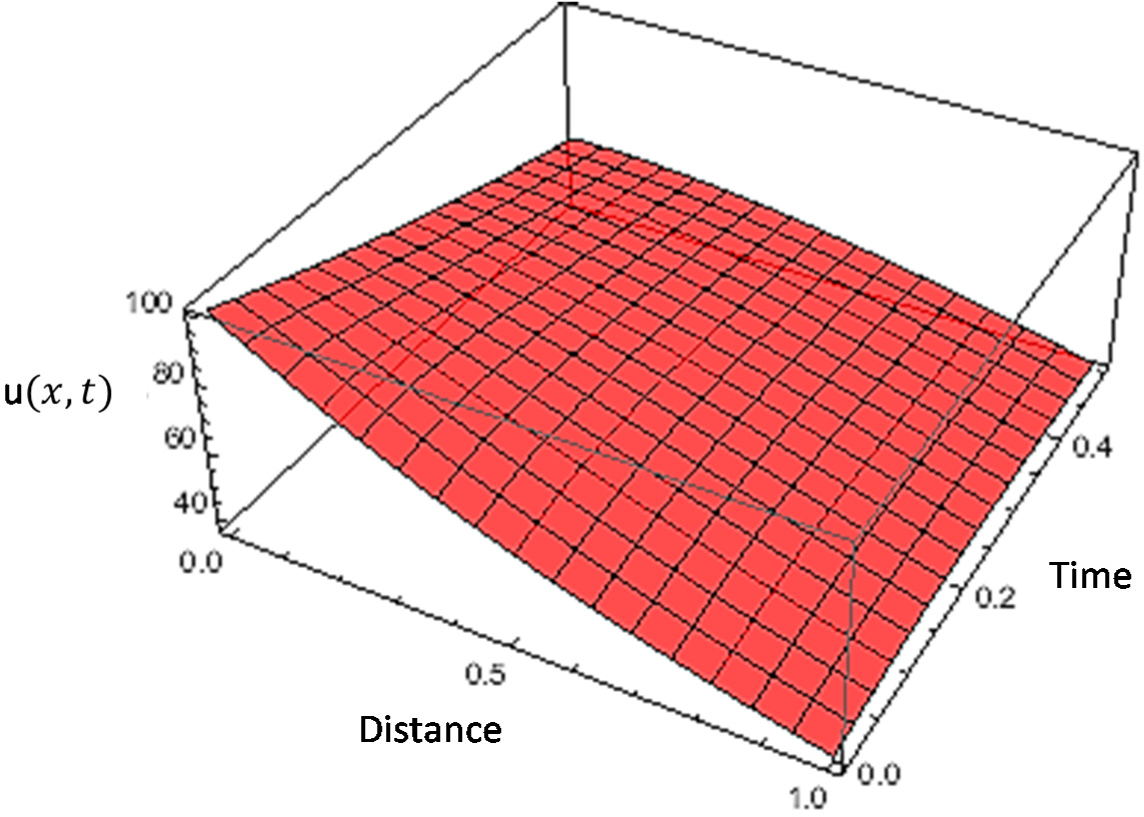
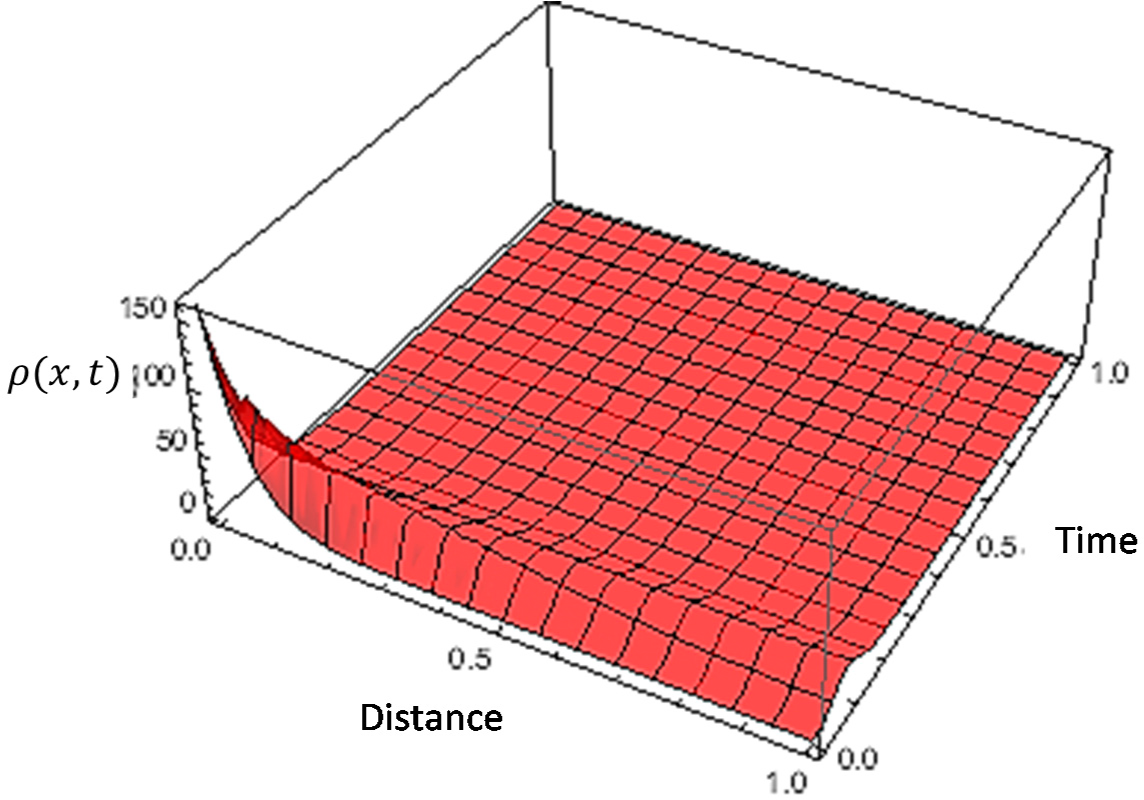
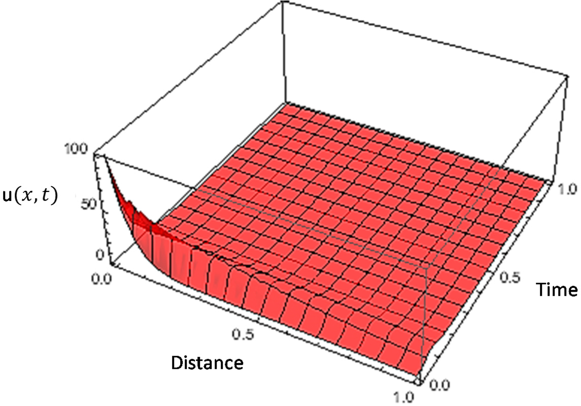
4. Derivation of Approximate Coupled-Solutions

Since the system is nonlinear and it may be hard to obtain the exact solution, in this section, we present the derivation of a special solution by employing an iterative technique. The technique involves coupling the Laplace transform and its inverse. Before presenting the methodology of the technique, we will first present the relationship between the Laplace transform and the new fractional derivative without singular kernel.

The connection between the Laplace transform and the Caputo-Fabrizio fractional order derivative is given as [12]:

$$ℒ\left({}_0{}^{CF}D{}_x^{\alpha }(f(x))\right)=\frac{pℒ\left(f(x)\right)-f(0)}{p+\alpha (1-p)}$$

(32)

Now applying the above operator on both sides of system (9) we obtain:

$$\{\begin{array}{c}\frac{pℒ\left(u(x,t)\right)-u(x,0)}{p+\alpha (1-p)}=ℒ\left\{a\frac{{\partial }^{2}u(x,t)}{\partial x^2}-\frac{\partial }{\partial x}\left(u(x,t)\frac{\partial \phi (\rho (x,t))}{\partial x}\right)\right\}\\ \frac{pℒ\left(\rho \left(x,t\right)\right)-\rho \left(x,0\right)}{p+\alpha (1-p)}=ℒ\left\{b\frac{{\partial }^2\rho (x,t)}{\partial x^2}+cu\left(x,t\right)-d\rho (x,t)\right\}\end{array}$$

(33)

We transform the above to:

$$\{\begin{array}{c}ℒ\left(u(x,t)\right)=\frac{u(x,0)}{p}+\frac{\left(p+\alpha (1-p)\right)}{p}ℒ\left\{a\frac{{\partial }^{2}u(x,t)}{\partial x^2}-\frac{\partial }{\partial x}\left(u(x,t)\frac{\partial \phi (\rho (x,t))}{\partial x}\right)\right\}\\ ℒ\left(\rho (x,t)\right)=\frac{\rho (x,0)}{p}+\frac{\left(p+\alpha (1-p)\right)}{p}ℒ\left\{b\frac{{\partial }^2\rho (x,t)}{\partial x^2}+cu\left(x,t\right)-d\rho (x,t)\right\}\end{array}$$

(34)

Now applying the inverse Laplace on both sides, we obtain:

$$\{\begin{array}{c}u\left(x,t\right)=u\left(x,0\right)+\\ {ℒ}^{-1}\left\{\frac{\left(p+\alpha (1-p)\right)}{p}ℒ\left\{a\frac{{\partial }^{2}u(x,t)}{\partial x^2}-\frac{\partial }{\partial x}\left(u(x,t)\frac{\partial \phi (\rho (x,t))}{\partial x}\right)\right\}\right\}\\ \rho \left(x,t\right)=\rho \left(x,0\right)+\\ {ℒ}^{-1}\left\{\frac{\left(p+\alpha (1-p)\right)}{p}ℒ\left\{b\frac{{\partial }^2\rho (x,t)}{\partial x^2}+cu\left(x,t\right)-d\rho (x,t)\right\}\right\}\end{array}$$

(35)

We assume the following iterative formula:

$$\{\begin{array}{c}{u}_{n+1}\left(x,t\right)=u_n\left(x,t\right)+\\ {ℒ}^{-1}\left\{\frac{\left(p+\alpha \left(1-p\right)\right)}{p}ℒ\left\{a\frac{{\partial }^2{u}_n\left(x,t\right)}{\partial x^2}-\frac{\partial }{\partial x}\left(u_n\left(x,t\right)\frac{\partial \phi \left({\rho }_n\left(x,t\right)\right)}{\partial x}\right)\right\}\right\}\\ {\rho }_{n+1}\left(x,t\right)={\rho }_n\left(x,t\right)+\\ {ℒ}^{-1}\left\{\frac{\left(p+\alpha \left(1-p\right)\right)}{p}ℒ\left\{b\frac{{\partial }^2{\rho }_n(x,t))}{\partial x^2}+c{u}_n\left(x,t\right)-d{\rho }_n\left(x,t\right)\right\}\right\}\end{array}$$

(36)

With the first component:

$$\{\begin{array}{l}{u}_0\left(x,t\right)=u(x,0)\\ {\rho }_0\left(x,t\right)=\rho \left(x,0\right)\end{array}$$

The coupled solution is thus provided as:

$$\{\begin{array}{l}u\left(x,t\right)=\underset{n\to \infty }{\lim }{u}_n(x,t)\\ \rho \left(x,t\right)=\underset{n\to \infty }{\lim }{\rho }_n(x,t)\end{array}$$

(37)

The numerical simulations are presented here for different values of alpha. The results are depicted in Figures 1–4.

From the above figures, one can see that the solution of our equation also depends on the fractional order. This shows that, the fractional order can be used to control the behavior of the solution in different scale within the system.

5. Conclusions

In this work, the aim was to check the possibility of extending the application of the new proposed fractional derivative without singular kernel to other fields of science. The original aim of the new derivative is the exploitation of the performance of the conventional viscoelastic materials, thermal media, electromagnetics system and others. We have applied the derivative to the Keller and Segel model and presented in detail the use of the fixed-point theorem to prove the existence and uniqueness of the coupled-solution. A derivation of the special solution was done via an iterative approach.