Binary Classification with a Pseudo Exponential Model and Its Application for Multi-Task Learning ^†

Abstract

In this paper, we investigate the basic properties of binary classification with a pseudo model based on the Itakura–Saito distance and reveal that the Itakura–Saito distance is a unique appropriate measure for estimation with the pseudo model in the framework of general Bregman divergence. Furthermore, we propose a novel multi-task learning algorithm based on the pseudo model in the framework of the ensemble learning method. We focus on a specific setting of the multi-task learning for binary classification problems. The set of features is assumed to be common among all tasks, which are our targets of performance improvement. We consider a situation where the shared structures among the dataset are represented by divergence between underlying distributions associated with multiple tasks. We discuss statistical properties of the proposed method and investigate the validity of the proposed method with numerical experiments.

1. Introduction

In the framework of multi-task learning problems, we assume that there are multiple related tasks (datasets) sharing a common structure and can utilize the shared structure to improve the generalization performance of classifiers for multiple tasks [1,2]. This framework has been successfully employed in various kind of applications, such as medical diagnosis. Most methods utilize the similarity among tasks to improve the performance of classifiers by representing the shared structure as a regularization term [3,4]. We tackle this problem using a boosting method, which makes it possible to adaptively learn complicated problems with low computational cost. The boosting methods are notable implementations of the ensemble learning and try to construct a better classifier by combining weak classifiers. AdaBoost is the most popular boosting method, and many variations, including TrAdaBoost for the multi-task learning [5], have been developed. In face recognition [6], as well as web search ranking [7], the computational efficiency of boosting is paid attention to in the framework of multi-task learning.

In this paper, we firstly reveal that AdaBoost can be derived by a sequential minimization of the Itakura–Saito (IS) distance between an empirical distribution and a pseudo measure model associated with a classifier. The IS distance is a special case of the Bregman divergence [8] between two positive measures and is frequently used for non-negative matrix factorization (NMF) in the region of signal processing [9,10]. Secondly, we propose a novel boosting algorithm for the multi-task learning based on the IS distance. We utilize the IS distance as a discrepancy measure between pseudo models associated with tasks and incorporate the IS distance as a regularizer into AdaBoost. The proposed method can capture the shared structure, i.e., the relationship between underlying distributions by considering the IS distance between pseudo models constructed by classifiers. We discuss the statistical properties of the proposed method and investigate the validity of the regularization by the IS distance with small experiments using synthetic datasets and a real dataset.

This paper is organized as follows. In Section 2, basic settings are described, and a divergence measure is introduced. In Section 3, we briefly introduce the IS distance, which is a special case of the Bregman divergence, and investigate the relationship between a well-known ensemble algorithm, AdaBoost and estimation with a pseudo model using the Itakura–Saito distance. In Section 4, we propose a method for multi-task learning, which is derived from a minimization of the weighted sum of divergence, and the performance of the proposed methods is examined in Section 5 using a synthetic dataset and a real dataset (a short version of this article has been presented as a conference paper [11]; some theoretical results and numerical experiments are added to the current version).

2. Settings

In this study, we focus on binary classification problems. Let x be an input and $y\in \mathrm{𝒴}=\{\pm 1\}$ be a class label. Let us assume that J datasets ${\mathrm{𝒟}}_j={\{x_i^{\left(j\right)},y_i^{\left(j\right)}\}}_{i=1}^{n_j}$ ($j=1,...,J$) are given, and let $p_j\left(y\right|x)r_j\left(x\right)$ and ${\tilde{p}}_j\left(y\right|x){\tilde{r}}_j\left(x\right)$ be an underlying distribution and an empirical distribution associated with the dataset ${\mathrm{𝒟}}_j$, respectively. Here, we assume that each conditional distribution of y given x is written as:

$$p_k\left(y\right|x)=p_0\left(y\right|x)+{\delta }_k\left(x\right)y$$

(1)

where $p_0\left(y\right|x)$ is a common conditional distribution for all datasets and ${\delta }_k\left(x\right)$ is a term that is specific to the dataset ${\mathrm{𝒟}}_k$. Note that ${\sum }_{y\in \mathrm{𝒴}}{\delta }_k\left(x\right)y=0$ holds, because $p_k\left(y\right|x)$ is a probability distribution. While a discriminant function $F_k$ is usually constructed using only the dataset ${\mathrm{𝒟}}_k$, the multi-task learning aims to improve the performance of the discriminant function for each dataset ${\mathrm{𝒟}}_k$ with the help of datasets ${\mathrm{𝒟}}_j$ ($j\ne k$). For this purpose, we consider a risk minimization problem defined with a pseudo model and the Itakura–Saito (IS) distance, which is a discrepancy measure frequently used in a region of signal processing.

Let $\mathrm{ℳ}=\left\{m\left(y\right)|0\le {\sum }_{y\in \mathrm{𝒴}}m\left(y\right)<\infty \right\}$ be a space of all positive finite measures over $𝒴$. The Itakura–Saito distance between $p,q\in \mathrm{ℳ}$ is defined as:

$$IS(p,q;r)=\int r\left(x\right)\sum _{y\in \mathrm{𝒴}}\left\{log\frac{q\left(y\right|x)}{p\left(y\right|x)}-1+\frac{p\left(y\right|x)}{q\left(y\right|x)}\right\}dx$$

(2)

where $r\left(x\right)$ is a marginal distribution of x shared by p, $q\in \mathrm{ℳ}$. Note that the IS distance is a kind of statistical version of the Bregman divergence [12], which makes it possible to directly plug-in the empirical distribution. We observe that $IS(p,q;r)\ge 0$ and $IS(p,q;r)=0$ if and only if $p=q$. banerjee et al. [13] showed that there exists a unique Bregman divergence corresponding to every regular exponential family, and the Itakura–Saito distance is associated with the exponential distribution.

3. Itakura–Saito Distance and Pseudo Model

3.1. Parameter Estimation with the Pseudo Model

Let $q_F\left(y\right|x)$ be an (un-normalized) pseudo model associated with a function $F\left(x\right)$,

$$q_F\left(y\right|x)=exp\left(F\left(x\right)y\right).$$

(3)

Note that $q_F\left(y\right|x)$ is not a probability function, i.e., ${\sum }_{y\in \mathrm{𝒴}}{q}_F\left(y\right|x)\ne 1$ in general. If $q_F\left(y\right|x)$ is normalized, the model reduces to the classical logistic model as:

$${\overline{q}}_F\left(y\right|x)=\frac{exp\left(F\right(x\left)y\right)}{exp\left(F\right(x\left)\right)+exp(-F(x\left)\right)}.$$

(4)

When the function F is parameterized by θ, the maximum likelihood estimation (MLE) ${\mathrm{argmax}}_{\theta }{\sum }_{i=1}^{n}log{\overline{q}}_F\left(y_i\right|x_i)$ or equivalently minimization of the (extended) Kullback–Leibler (KL) divergence is a powerful tool for the estimation of θ, and the MLE has properties such as asymptotic consistency and efficiency under some regularity conditions. Here, we consider parameter estimation with the pseudo model Equation (3) rather than the normalized model Equation (4).

Proposition 1. Let $p\left(y\right|x)={\overline{q}}_{F_0}\left(y\right|x)$ be the underlying distribution. Then, we observe:

$$\begin{array}{cc}\hfill \underset{F}{\mathrm{argmin}}IS(p,q_F;r)& =F_0,\hfill \end{array}$$

(5)

$$\begin{array}{cc}\hfill \underset{F}{\mathrm{argmin}}IS(q_F,p;r)& =F_0.\hfill \end{array}$$

(6)

Proof. See Appendix A

On the other hand, when we consider an estimation based on the extended KL divergence, i.e., ${\mathrm{argmin}}_{F}KL(p,q_F;r)$ where:

$$KL(p,q;r)=\int r\left(x\right)\sum _{y\in \mathrm{𝒴}}\{p\left(y\right|x)log\frac{p\left(y\right|x)}{q\left(y\right|x)}-p\left(y\right|x)+q\left(y\right|x)\}dx,$$

(7)

we observe the following.

Proposition 2. Let $F_0$ be a function $F_0$($\ne 0$) and $p\left(y\right|x)={\overline{q}}_{F_0}\left(y\right|x)$ be the underlying distribution. Then, we observe:

$$\begin{array}{cc}\hfill F_{KL,1}=\underset{F}{\mathrm{argmin}}KL(p,q_F;r)\ne & F_0,\hfill \end{array}$$

(8)

$$\begin{array}{cc}\hfill F_{KL,2}=\underset{F}{\mathrm{argmin}}KL(q_F,p;r)\ne & F_0.\hfill \end{array}$$

(9)

Proof. See Appendix B.

Remark 1. Let $p\left(y\right|x)={\overline{q}}_{F_0}\left(y\right|x)$ be the underlying distribution. Then, minimizer Equation (8) or (9) of the extended KL divergence attains the Bayes rule, i.e.,

$$\begin{array}{cc}\hfill sgn\left(F_{KL,1}\left(x\right)\right)& =sgn\left(F_{KL,2}\left(x\right)\right)=sgn\left(\frac{1}{2}log\frac{p(+1|x)}{p(-1|x)}\right).\hfill \end{array}$$

(10)

The proposition and the remark show that the extended KL divergence is not completely appropriate for estimation with the pseudo model.

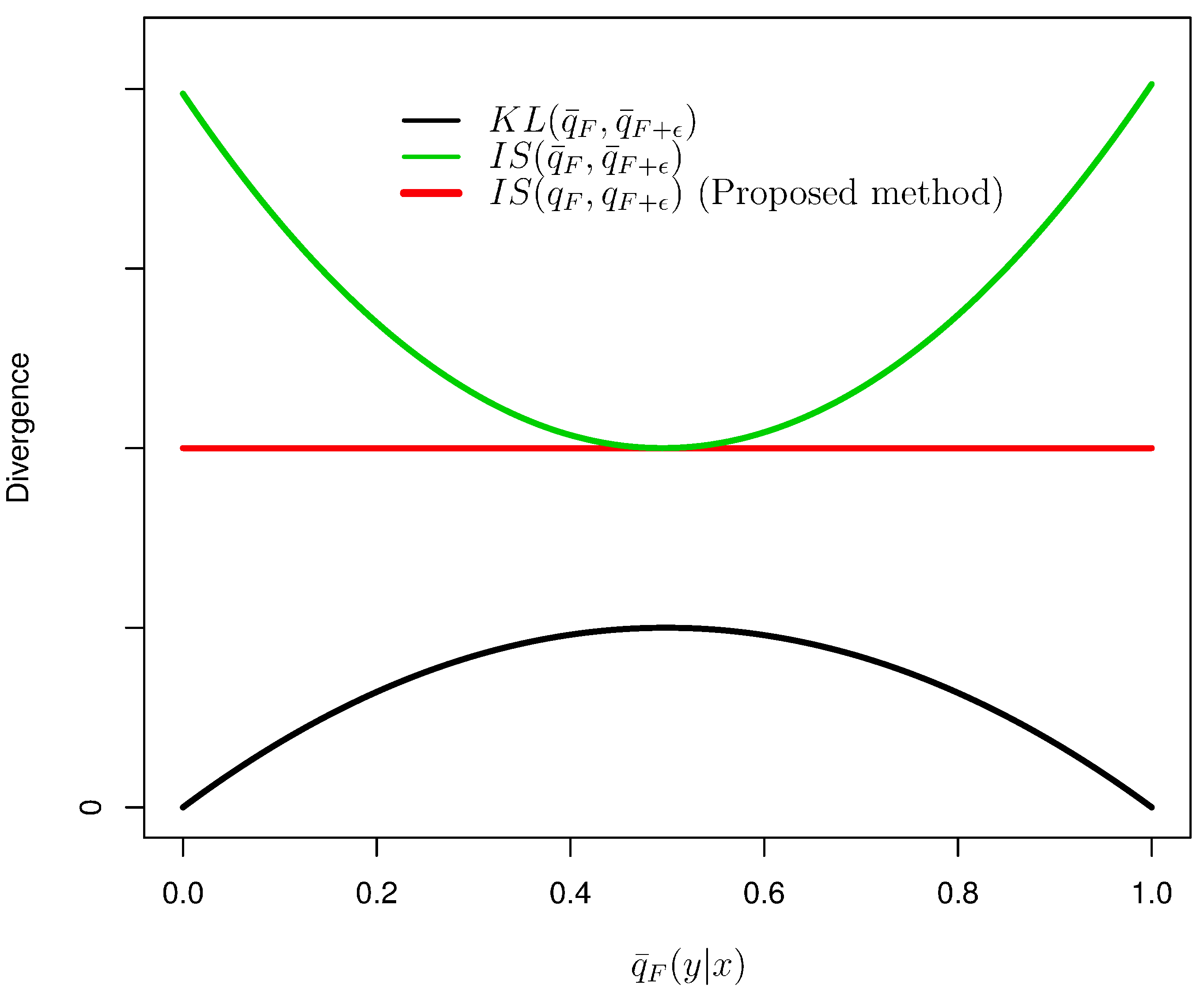
3.2. Characterization of the Itakura–Saito Distance

In this section, we investigate the characterization of the Itakura–Saito distance for estimation with the pseudo model, in the framework of the Bregman U-divergence. Firstly, we briefly introduce the statistical version of Bregman U-divergence [12]. The statistical version of Bregman U-divergence is a discrepancy measure between positive measures in $ℳ$ defined by a generating function U and enables us to directly plug-in the empirical distribution for estimation. [12] proposed a general boosting-type algorithm for classification using the Bregman U-divergence and discussed properties of the method from the viewpoint of information geometry [14]. By changing the generating function U, the Bregman U-divergence can have a useful property as robustness against noise. For example, the β-divergence is a special case of the Bregman U-divergence and is frequently used for robust estimation in the context of unsupervised learning, such as clustering or component analysis [15,16]. Another example of the Bregman U-divergence is the η-divergence, which is employed to robustify the classification algorithm and is closely related to probability models of mislabeling [17,18].

Let U be a monotonically-increasing convex function and ξ be an inverse function of $U^{\prime }$, the derivative of U. From the convexity of the function U, the function ξ is a monotonically-increasing function. The statistical version of Bregman U-divergence between two measures $p,q\in \mathrm{ℳ}$ is defined as follows.

$$\begin{array}{c}\hfill D_U(p,q;r)=\int r\left(x\right)\sum _{y\in \mathrm{𝒴}}\left\{U\left(\xi \left(q\left(y\right|x)\right)\right)-U\left(\xi \left(p\left(y\right|x)\right)\right)-p\left(y\right|x)\left(\xi \left(q\right(y\left|x\right))-\xi (p\left(y\right|x\left)\right)\right)\right\}dx.\end{array}$$

(11)

Note that the function ξ should be defined at least on $z>0$.

Remark 2. The KL divergence and the Itakura–Saito distance are special cases of the Bregman U-divergence Equation (11) with generating functions $U\left(z\right)=exp\left(z\right)$ and $U\left(z\right)=-log(c-z)+c_1$ ($z<c$), where c and $c_1$ are constants, respectively.

Here, we introduce the concept of reflection-symmetric for characterization of the IS distance.

Definition 3. A function $f\left(z\right)$ is reflection-symmetric if:

$$\begin{array}{c}\hfill f\left(z\right)=f\left(z^{-1}\right)\end{array}$$

(12)

holds for all $z\ne 0$.

If the function f is reflection-symmetric, we observe that:

$$\begin{array}{c}\hfill \underset{z\to 0}{lim}f\left(z\right)=\underset{z\to \infty }{lim}f\left(z\right).\end{array}$$

(13)

Because of this property, the reflection-symmetric function often has a singular point at $z=0$, and to investigate the behavior of the function, we can employ the Laurent series as:

$$\begin{array}{c}\hfill f\left(z\right)=c+\sum _{k=1}^{\infty }\left(a_k{z}^k+b_k{z}^{-k}\right).\end{array}$$

(14)

Note that if the function f is holomorphic over R, $b_k=0$ for all k, and the Laurent series is equivalent to the Taylor series.

Remark 3. If the function f is reflection-symmetric and holomorphic over R, $a_k=b_k=0$ holds for all k, and then, f is a constant function.

For the Bregman U-divergence Equation (11), we observe the following Lemma.

Lemma 4. Let $F_0$ be an arbitrary function, $p\left(y\right|x)={\overline{q}}_{F_0}\left(y\right|x)$ be the underlying distribution and $q_F\left(x\right)$ be the pseudo model Equation (3). If the Bregman U-divergence associated with the function U attains:

$$\begin{array}{c}\hfill F_0=\underset{F}{\mathrm{argmin}}{D}_U(p,q_F;r),\end{array}$$

(15)

a function ${\xi }^{\prime }\left(z\right)z^2$ derived from U is reflection-symmetric. In addition, if the Bregman U-divergence associated with the function U attains:

$$\begin{array}{c}\hfill F_0=\underset{F}{\mathrm{argmin}}{D}_U(q_F,p;r),\end{array}$$

(16)

a function $z\left\{\xi \left(z\right)-\xi \left(\frac{z}{z+z^{-1}}\right)\right\}$ derived from U is reflection-symmetric.

Proof. See Appendix C.

Remark 4. Proposition 1 implies that the function ξ associated with the IS distance satisfies Lemma 4.

Remark 5. Propositions imply that the function U, i.e., Bregman U-divergence, attains Equation (15) or (16) is not unique and there exists divergences satisfying Equation (15) or (16), other than the Itakura–Saito distance. For example, a function:

$$\begin{array}{c}\hfill \xi \left(z\right)=-2z^{-\frac{2}{3}}-z^{-\frac{4}{3}}\end{array}$$

(17)

satisfies ${\xi }^{\prime }\left(z\right)z^2=\frac{4}{3}(z^{1/3}+z^{-1/3})$, and then, ${\xi }^{\prime }\left(z\right)z^2$ is reflection-symmetric. The associated generating function U is written as:

$$\begin{array}{cc}\hfill U\left(z\right)& ={\int }^z{\xi }^{-1}\left(z^{\prime }\right)d{z}^{\prime }=-4\frac{-2+\sqrt{1-z}}{\sqrt{-1+\sqrt{1-z}}}+C_1\hfill \end{array}$$

(18)

where $C_1$ is a constant.

In the following theorem, we reveal the characterization of the Itakura–Saito distance for estimation with the pseudo model Equation (3) and the Bregman U-divergence.

Theorem 5. Let $p\left(y\right|x)={\overline{q}}_{F_0}\left(y\right|x)$ be the underlying distribution and $q_F\left(x\right)$ be the pseudo model Equation (3). If conditions:

$$\begin{array}{cc}\hfill F_0& =\underset{F}{\mathrm{argmin}}{D}_U(p,q_F;r),\hfill \end{array}$$

(19)

$$\begin{array}{cc}\hfill F_0& =\underset{F}{\mathrm{argmin}}{D}_U(q_F,p;r)\hfill \end{array}$$

(20)

simultaneously hold, then $U\left(z\right)=-log(-z)$, i.e., $D_U(p,q;r)$ is the Itakura–Saito distance $IS(p,q;r)$.

Proof. See Appendix D.

Remark 6. If we assume that a function ${\xi }^{\prime }\left(z\right)z^2$ derived from U is reflection-symmetric and holomorphic over R, ${\xi }^{\prime }\left(z\right)z^2$ is a constant function from Remark 3. Then, we obtain $\xi \left(z\right)=c+\frac{b_1}{z}$ where $c,b_1$ are constants, implying that the associated divergence is equivalent to the Itakura–Saito distance.

3.3. Relationship with AdaBoost

The IS distance between the underlying conditional distribution $p\left(y\right|x)$ and the pseudo model $q_F\left(y\right|x)$ is written as:

$$\begin{array}{cc}\hfill IS(p,q_F;r)& =C+\int r\left(x\right)\sum _{y\in \mathrm{𝒴}}\left\{F\left(x\right)y+\frac{p\left(y\right|x)}{q_F\left(y\right|x)}\right\}dx\hfill \\ & =C+\int r\left(x\right)\sum _{y\in \mathrm{𝒴}}p\left(y\right|x)e^{-F\left(x\right)y}dx,\hfill \end{array}$$

(21)

where C is a constant, and Equation (21) is equivalent to an expected loss of AdaBoost, except for the constant term. Then, sequential minimization of an empirical version of Equation (21) is equivalent to the algorithm of AdaBoost, which is the most popular boosting method for the binary classification. Furthermore, [12,19] discussed that a gradient-based boosting algorithm can be derived from the minimization of the KL divergence or the Bregman U-divergence between the underlying distribution and a pseudo model. An important difference between these frameworks and our framework Equation (21) is the employed pseudo model. The pseudo model employed by the previous frameworks assumes a condition called “consistent data assumption” and is defined with the empirical distribution, implying that the pseudo model varies depending on the dataset. On the other hand, the pseudo model Equation (3) employed in Equation (21) is fixed against the dataset as usual statistical models.

The IS distance between two pseudo models $q_F\left(y\right|x)$ and $q_{F^{\prime }}\left(y\right|x)$ is written as,

$$\begin{array}{cc}\hfill IS(q_F,q_{F^{\prime }};r)& =\int r\left(x\right)\sum _{y\in \mathrm{𝒴}}\left\{F^{\prime }\left(x\right)y-F\left(x\right)y-1+exp(F\left(x\right)y-F^{\prime }\left(x\right)y)\right\}dx\hfill \\ & =2+\int r\left(x\right)\left\{exp(F\left(x\right)-F^{\prime }\left(x\right))+exp(F^{\prime }\left(x\right)-F\left(x\right))\right\}dx.\hfill \end{array}$$

(22)

Note that $IS(q_{F^{\prime }},q_F;r)=IS(q_F,q_{F^{\prime }};r)$ holds for arbitrary $q_F$ and $q_{F^{\prime }}$, while the IS distance itself is not necessarily symmetric. Furthermore, note that the symmetric property does not hold for normalized models ${\overline{q}}_F$ and ${\overline{q}}_{F^{\prime }}$.

4. Application for Multi-Task Learning

There are two main types of frameworks for multi-task learning [20,21].

Case 1 :

There is a target dataset ${\mathrm{𝒟}}_k$, and our interest is to construct a discriminant function $F_k$ utilizing remaining datasets ${\mathrm{𝒟}}_j$ ($j\ne k$) or a priori constructed discriminant functions $F_j$ ($j\ne k$).

Case 2 :

Our interest is to simultaneously construct better discriminant functions $F_1,...,F_J$ using all J datasets ${\mathrm{𝒟}}_1,...,{\mathrm{𝒟}}_J$ by utilizing shared information among datasets.

4.1. Case 1

In this section, we focus on the above first framework. Let us assume that discriminant functions $F_j\left(x\right)$ ($j\ne k$) are given or are constructed by an arbitrary binary classification method. Then, let us consider a risk function:

$$\begin{array}{cc}\hfill L_k\left(F_k\right)=& IS(p_k,q_{F_k};r_k)+\sum _{j\ne k}{\text{λ}}_{k,j}IS(q_{F_k},q_{F_j};r_k)\hfill \\ \hfill =& \int r_k\left(x\right)\left\{\sum _{y\in \mathrm{𝒴}}{p}_k\left(y\right|x)e^{-F_k\left(x\right)y}+\sum _{j\ne k}{\text{λ}}_{k,j}\left\{e^{F_k\left(x\right)-F_j\left(x\right)}+e^{F_j\left(x\right)-F_k\left(x\right)}\right\}\right\}dx,\hfill \end{array}$$

(23)

where ${\text{λ}}_{k,j}\ge 0$ ($j\ne k$) are regularization constants. Note that the risk function depends on functions $F_j$ ($j\ne k$), and the second term becomes small when the target discriminant function $F_k$ is similar to functions $F_j$($j\ne k$) in the sense of the IS distance; and the second term corresponds to a regularizer incorporating the shared information among datasets into the target function $F_k$. Furthermore, note that the marginal distribution $r_k$ is shared in the second term for the ease of implementation and the simplicity of theoretical analysis.

An empirical version of Equation (23) is written as:

$${\overline{L}}_k\left(F_k\right)=\frac{1}{n_k}\sum _{i=1}^{n_k}\left(e^{-F_k\left(x_i^{\left(k\right)}\right)y_i^{\left(k\right)}}+\sum _{j\ne k}{\lambda }_{k,j}\left(e^{F_k\left(x_i^{\left(k\right)}\right)-F_j\left(x_i^{\left(k\right)}\right)}+e^{F_j\left(x_i^{\left(k\right)}\right)-F_k\left(x_i^{\left(k\right)}\right)}\right)\right).$$

(24)

An algorithm is derived by sequential minimization of Equation (24) by updating $F_k$ to $F_k+\alpha f$, i.e., $(\alpha ,f)={\mathrm{argmin}}_{\alpha ,f}{\overline{L}}_k(F_k+\alpha f)$, where f is a weak classifier and α is a coefficient [22].

(1)

Initialize the function to $F_k^0$, and define weights for the i-th example with a function F as:

$$\begin{array}{cc}\hfill w_1(i;F)& =\frac{e^{-F\left(x_i^{\left(k\right)}\right)y_i^{\left(k\right)}}}{Z_1\left(F\right)},\hfill \\ \hfill w_2(i;F)& =\frac{{\sum }_{j\ne k}{\lambda }_{k,j}{e}^{f\left(x_i^{\left(k\right)}\right)(F\left(x_i^{\left(k\right)}\right)-F_j\left(x_i^{\left(k\right)}\right))}}{Z_2\left(F\right)}\hfill \end{array}$$

where:

$$\begin{array}{cc}\hfill Z_1\left(F\right)& =\sum _{i=1}^{n_k}{e}^{-F\left(x_i^{\left(k\right)}\right)y_i^{\left(k\right)}},\hfill \\ \hfill Z_2\left(F\right)& =\sum _{i=1}^{n_k}\sum _{j\ne k}{\lambda }^{k,j}\left(e^{F\left(x_i^{\left(k\right)}\right)-F_j\left(x_i^{\left(k\right)}\right)}+e^{-F\left(x_i^{\left(k\right)}\right)+F_j\left(x_i^{\left(k\right)}\right)}\right).\hfill \end{array}$$

(2)

For $t=1,...,T$

(a)

Select a weak classifier $f_k^t\in \{\pm 1\}$, which minimizes the following quantity:

$$\epsilon \left(f\right)=\frac{Z_1\left(F_k^{t-1}\right)}{Z_1\left(F_k^{t-1}\right)+Z_2\left(F_k^{t-1}\right)}{\epsilon }_1\left(f\right)+\frac{Z_2\left(F_k^{t-1}\right)}{Z_1\left(F_k^{t-1}\right)+Z_2\left(F_k^{t-1}\right)}{\epsilon }_2\left(f\right).$$

(25)

where ${\epsilon }_1\left(f\right)={\sum }_{i=1}^{n_k}{w}_1(i;F_k^{t-1})I(f\left(x_i^{\left(k\right)}\right)\ne y_i^{\left(k\right)})$ and ${\epsilon }_2\left(f\right)={\sum }_{i=1}^n{w}_2(i;F_k^{t-1})$.

(b)

Calculate a coefficient of $f_k^t$ by ${\alpha }_k^t=\frac{1}{2}log\frac{1-\epsilon \left(f_k^t\right)}{\epsilon \left(f_k^t\right)}$.

(c)

Update the discriminant function as $F_k^t=F_k^{t-1}+{\alpha }_k^t{f}_k^t$.

(3)

Output $F_k^T\left(x\right)=F_k^0\left(x\right)+{\sum }_{t=1}^T{\alpha }_k^t{f}_k^t\left(x\right)$.

In Step 1, $F_k^0$ is typically initialized as $F_k^0\left(x\right)=0$. The quantity Equation (25) is a mixture of two terms: ${\epsilon }_1\left(f\right)$ is a weighted error rate of the classifier f, and ${\epsilon }_2\left(f\right)$ is the sum of weights $w_2\left(f\right)$, which represents the degree of discrepancy between f and $F-F_j$. ${\epsilon }_2\left(f\right)$ becomes large when F is updated by f as departed from $F_j$. Note that if we set ${\lambda }_{k,j}=0$ for all j, the risk function Equation (24) coincides with that of AdaBoost, and the above derived algorithm reduces to the usual AdaBoost.

Because the empirical risk function Equation (24) is convex with respect to F or $F^{\prime }$, we can consider another version of the risk function as:

$$\begin{array}{cc}\hfill {\overline{L}}_k\left(F_k\right)& =\frac{1}{n_k}\sum _{i=1}^{n_k}\left(e^{-F_k\left(x_i^{\left(k\right)}\right)y_i^{\left(k\right)}}+{\lambda }_k\left(e^{F_k\left(x_i^{\left(k\right)}\right)-{\overline{F}}_k\left(x_i^{\left(k\right)}\right)}+e^{-F_k\left(x_i^{\left(k\right)}\right)+{\overline{F}}_k\left(x_i^{\left(k\right)}\right)}\right)\right)\hfill \end{array}$$

(26)

where ${\overline{F}}_k\left(x\right)={\sum }_{j\ne k}\frac{{\lambda }_{k,j}}{{\lambda }_k}{F}_j\left(x\right)$. The risk function is upper bounded by the risk function Equation (24), implying that the effect of regularization by the shared information is weakened. The derived algorithm is almost the same as the one derived from Equation (24).

4.2. Case 2

In this section, we consider simultaneous construction of discriminant functions $F_1,...,F_J$ by minimizing the following risk function:

$$L(F_1,...,F_J)=\sum _{j=1}^J{\pi }_j{L}_j\left(F_j\right)$$

(27)

where ${\pi }_j$($j=1,...,J$) is a positive constant satisfying ${\sum }_{j=1}^J{\pi }_j=1$ and $L_k$ is defined in Equation (23).

Though we can directly minimize the empirical version of Equation (27), a derived algorithm is complicated and is computationally heavy. Then, we derive a simplified algorithm utilizing the algorithm shown in Case 1 in which a target dataset is fixed.

(1)

Initialize functions $F_1,...,F_J$.

(2)

For $t=1,...,T$:

(a)

Randomly choose a target index $k\in \{1,...,J\}$.

(b)

Update the function $F_k$ using the algorithm in Case 1 by S steps, with fixed functions $F_j$ ($j\ne k$).

(3)

Output learned functions $F_1,...,F_J$.

Note that the empirical risk function cannot be monotonically decreased because the minimization of $L_k\left(F_k\right)$ is a trade-off of the first term and the second regularization term, and a decrease of $L_k\left(F_k\right)$ does not necessarily mean a decrease of the regularization term.

4.3. Statistical Properties of the Proposed Methods

In this section, we discuss the statistical properties of the proposed methods. Firstly, we focus on Case 1, and the minimizer $F_k^{*}$ of the risk function Equation (23) satisfies the following:

$$\begin{array}{cc}\hfill {\left.\frac{\delta L_k\left(F_k\right)}{\delta F_k\left(x\right)}\right|}_{F_k=F_k^{*}}& \propto -p_k(+1|x)e^{-F_k^{*}\left(x\right)}+p_k(-1|x)e^{F_k^{*}\left(x\right)}+\sum _{j\ne k}{\lambda }_{k,j}\left\{e^{F_k^{*}\left(x\right)-F_j\left(x\right)}-e^{F_j\left(x\right)-F_k^{*}\left(x\right)}\right\}=0,\hfill \end{array}$$

(28)

which implies:

$$\begin{array}{cc}\hfill F_k^{*}\left(x\right)& =\frac{1}{2}log\frac{p_k(+1|x)+{\sum }_{j\ne k}{\lambda }_{k,j}exp\left(F_j\left(x\right)\right)}{p_k(-1|x)+{\sum }_{j\ne k}{\lambda }_{k,j}exp(-F_j\left(x\right))},\hfill \end{array}$$

(29)

or equivalently:

$$\begin{array}{cc}\hfill p_k\left(y\right|x)& =p_{0,k}\left(y\right|x)\left(1+\sum _{j\ne k}{\lambda }_{k,j}exp(-F_j\left(x\right)y)\right)-p_{0,k}(-y|x)\sum _{j\ne k}{\lambda }_{k,j}exp\left(F_j\left(x\right)y\right),\hfill \end{array}$$

(30)

where $p_{0,k}\left(y\right|x)=\frac{exp\left(F_k^{*}\left(x\right)y\right)}{exp\left(F_k^{*}\left(x\right)\right)+exp(-F_k^{*}\left(x\right))}$. This can be interpreted as a probabilistic model of asymmetric mislabeling [17,18]. In Equation (29), the confidence of classification is discounted by the results of remaining discriminant functions when the classifier $sgn\left(F_k^{*}\left(x\right)\right)$ makes a different decision from these of $sgn\left(F_j\left(x\right)\right)$ ($j\ne k$).

Remark 7. $F_k^{*}\left(x\right)\ge 0$ does not mean $p_k(+1|x)\ge \frac{1}{2}$ unless $F_j\left(x\right)=\frac{1}{2}log\frac{p_k(+1|x)}{p_k(-1|x)}$ holds.

Proposition 6. Let us assume that $F_j\left(x\right)$ satisfies:

$$\frac{exp\left(F_j\left(x\right)y\right)}{exp\left(F_j\left(x\right)\right)+exp(-F_j\left(x\right))}=p_0\left(y\right|x)+{ϵ}_j\left(x\right)y,\left|\right|{ϵ}_j\left(x\right)\left|\right|\ll 1.$$

(31)

Then, Equation (29) can be approximated as:

$$F_k^{*}\left(x\right)\simeq \frac{1}{2}log\frac{p_0(+1|x)}{p_0(-1|x)}+\frac{1}{2P^2}\frac{P{\delta }_k\left(x\right)+{\sum }_{j\ne k}{\lambda }_{k,j}{ϵ}_j\left(x\right)}{P+{\lambda }_k}$$

(32)

where $P=\sqrt{p_0(+1|x)p_0(-1|x)}$ and ${\lambda }_k={\sum }_{j\ne k}{\lambda }_{k,j}$.

Proof. We obtain Equation (32) by considering the Taylor expansion of Equation (29).

We observe that a discrepancy derived by ${\delta }_k$ is moderated by the mixture of ${ϵ}_j$ when perturbations ${ϵ}_j$ are independently and identically distributed.

Proposition 7. Let ${\eta }_j\left(x\right)=F_j\left(x\right)-F_k\left(x\right)$ be a difference between two functions. Then, $F_k^{*}$ can be approximated as:

$$\begin{array}{c}\hfill F_k^{*}\left(x\right)\simeq \frac{1}{2}log\frac{p_k(+1|x)}{p_k(-1|x)}+\frac{1}{P}\sum _{j\ne k}{\lambda }_{k,j}{\eta }_j\left(x\right).\end{array}$$

(33)

Proof. See Appendix E.

Proposition 8. Let ${\overline{F}}_k^{*}$ be a minimizer of the risk function Equation (23) with ${\lambda }_{k,j}=0$($j\ne k$). Then, we observe:

$$\begin{array}{cc}\hfill {\left({\overline{F}}_k^{*}\left(x\right)-\frac{1}{2}log\frac{p_0(+1|x)}{p_0(-1|x)}\right)}^2& \ge {\left(F_k^{*}\left(x\right)-\frac{1}{2}log\frac{p_0(+1|x)}{p_0(-1|x)}\right)}^2,\hfill \end{array}$$

(34)

i.e., the proposed method improves the performance in the sense of the squared error, when:

$$|{\delta }_k(x)|\ge \frac{|{\sum }_{j\ne k}{\lambda }_{k,j}{ϵ}_j\left(x\right)|}{{\lambda }_k}$$

(35)

holds.

Proof. See Appendix F.

Secondly, we consider a property of the algorithm for Case 2.

Proposition 9. Let $r\left(x\right)=r_j\left(x\right)$ ($j=1,...,J$) be a common marginal distribution shared by all tasks. Then, the minimizer of the risk function is written as:

$$\begin{array}{cc}\hfill F_k\left(x\right)& =\frac{1}{2}log\frac{p_k(+1|x)+{\sum }_{j\ne k}{\lambda }_{jk}{e}^{F_j\left(x\right)}}{p_k(-1|x)+{\sum }_{j\ne k}{\lambda }_{jk}{e}^{-F_j\left(x\right)}},\hfill \end{array}$$

(36)

where ${\lambda }_{jk}={\lambda }_{k,j}+\frac{{\pi }_j}{{\pi }_k}{\lambda }_{k,j}$.

Proof. See Appendix G.

The only difference from Equation (28) is that regularization is strengthened by $\frac{{\pi }_j}{{\pi }_k}{\lambda }_{k,j}$, and then, the same propositions in Section 4.1 hold for Equation (36).

4.4. Comparison of Regularization Terms

The proposed method incorporates the regularization term defined by the IS distance into AdaBoost. In this section, we discuss a property of the regularization term.

Proposition 10. Let $ϵ\left(x\right)$ be a perturbation function satisfying $\left|ϵ\right(x\left)\right|\ll 1$. Then, we observe:

$$\begin{array}{cc}\hfill KL({\overline{q}}_F,{\overline{q}}_{F+ϵ};r)& \simeq \int 2r\left(x\right)ϵ{\left(x\right)}^2{\overline{q}}_F(+1|x){\overline{q}}_F(-1|x)dx,\hfill \end{array}$$

(37)

$$\begin{array}{cc}\hfill KL(q_F,q_{F+ϵ};r)& \simeq \int \frac{r\left(x\right)}{2}ϵ{\left(x\right)}^2\frac{1}{\sqrt{{\overline{q}}_F(+1|x){\overline{q}}_F(-1|x)}}dx,\hfill \end{array}$$

(38)

$$\begin{array}{cc}\hfill IS({\overline{q}}_F,{\overline{q}}_{F+ϵ};r)& \simeq \int 2r\left(x\right)ϵ{\left(x\right)}^2\sum _{y\in \mathrm{𝒴}}{\overline{q}}_F{\left(y\right|x)}^{2}dx,\hfill \end{array}$$

(39)

$$\begin{array}{cc}\hfill IS(q_F,q_{F+ϵ};r)& \simeq \int r\left(x\right)ϵ{\left(x\right)}^{2}dx.\hfill \end{array}$$

(40)

Proof. We obtain these approximations by considering the Taylor expansion up to second order.

Figure 1. Values of divergences (regularization terms) against ${\overline{q}}_F$.

Figure 1. Values of divergences (regularization terms) against ${\overline{q}}_F$.

Figure 1 shows values of divergences against a value of ${\overline{q}}_F\left(x\right)$. Those relations implies that the KL divergence Equation (37) emphasizes a region of input x whose conditional distribution ${\overline{q}}_F\left(x\right)$ is nearly equal to $\frac{1}{2}$, i.e., the classification boundary, while the IS distance Equation (39) focuses on a region of x whose conditional distribution is nearly equal to zero or one. The IS distance between pseudo model Equation (40), i.e., the proposed method, considers the intermediate of Equations (37) and (39). This implies that the regularization Equation (40) with the IS distance puts more focus on a region far from the classification boundary compared to Equation (37), while Equation (39) tends to relatively ignore the region near the classification boundary. Furthermore, note that the employment of Equation (40) makes it possible to derive the simple algorithm shown in Section 4.1.

5. Experiments

In this section, we investigate the performance of the proposed multi-task algorithm with synthetic datasets and a real dataset.

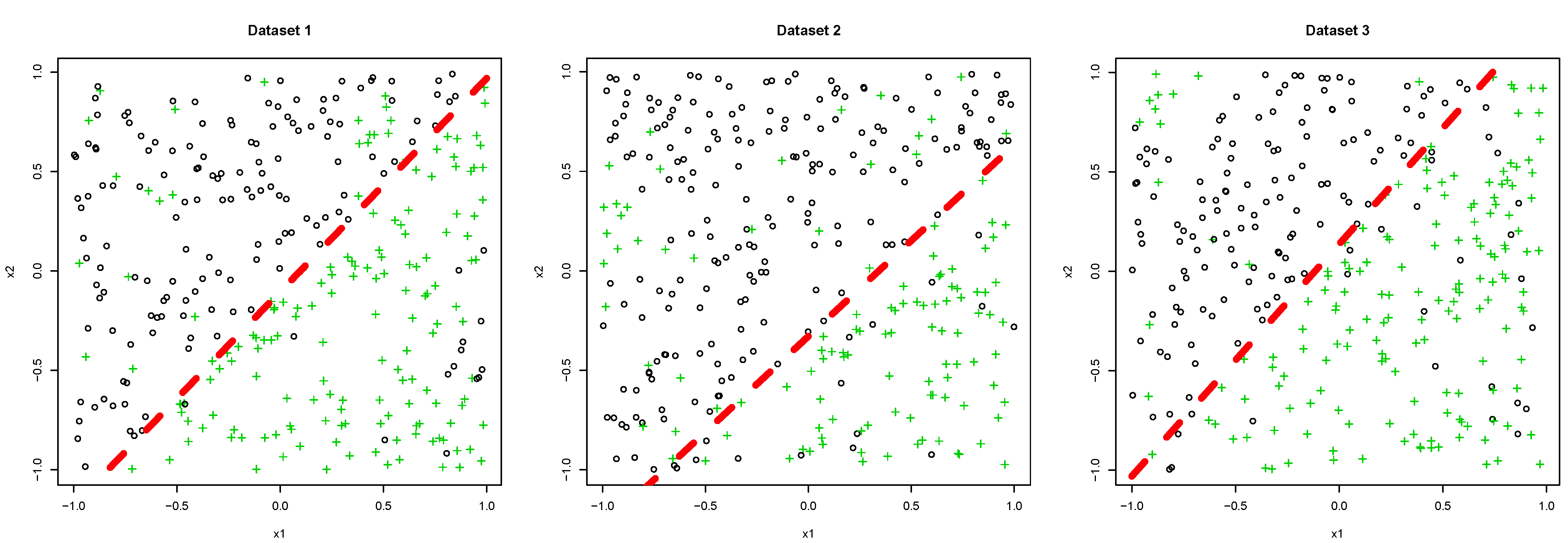
5.1. Synthetic Dataset

Firstly, we investigate the performance of the proposed method using two synthetic datasets within the situation described in Case 2. We compared the proposed method with AdaBoost trained with an individual dataset and AdaBoost trained with all datasets simultaneously. We employed the boosting stump (the boosting stump is a decision tree with only one node) as the weak classifier and fixed as ${\pi }_j=1/J$. A boosting-type method has a hyper-parameter T, the step number of boosting, and the proposed method additionally has the hyper-parameter ${\lambda }_{k,j}$. In the experiment, we determined these parameters T and ${\lambda }_{k,j}$ by the validation technique. Especially, we investigated two kinds of scenarios for the determination of ${\lambda }_{k,j}$.

• We set that ${\lambda }_{k,j}=\lambda$ for all $j,k$ and determined λ.
• We set that ${\lambda }_{k,j}=\frac{\lambda }{IS\left(q_{{\widehat{F}}_k},q_{{\widehat{F}}_j};r_k\right)}$ where ${\widehat{F}}_j$ is a discriminant function constructed by AdaBoost with the dataset ${\mathrm{𝒟}}_j$ and determined λ.

Scenario 2 can incorporate more detailed information about the relationship between tasks, and the proposed method can ignore the information of tasks having less shared information. In summary, we compared the following four methods:

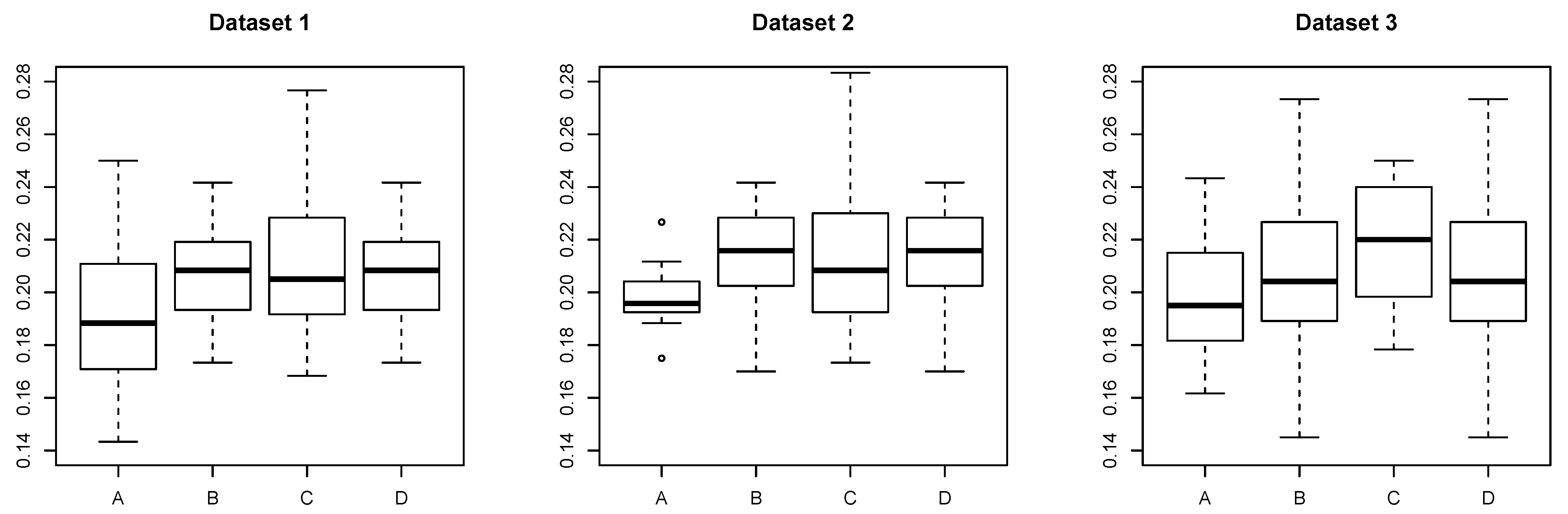
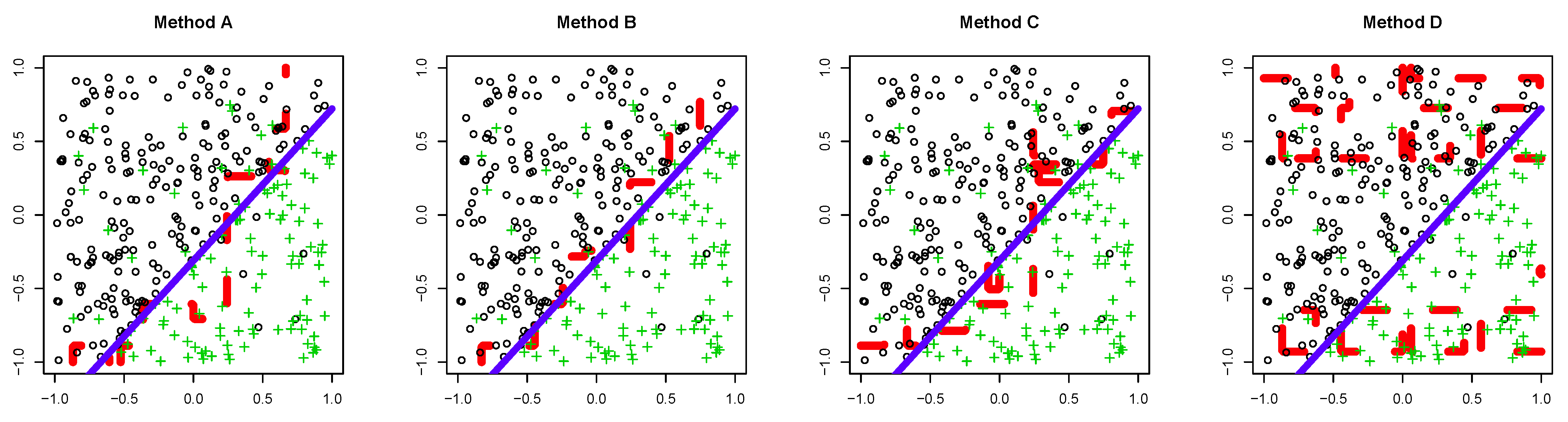
A:

The proposed method with ${\lambda }_{k,j}$ determined by Scenario 1.

B:

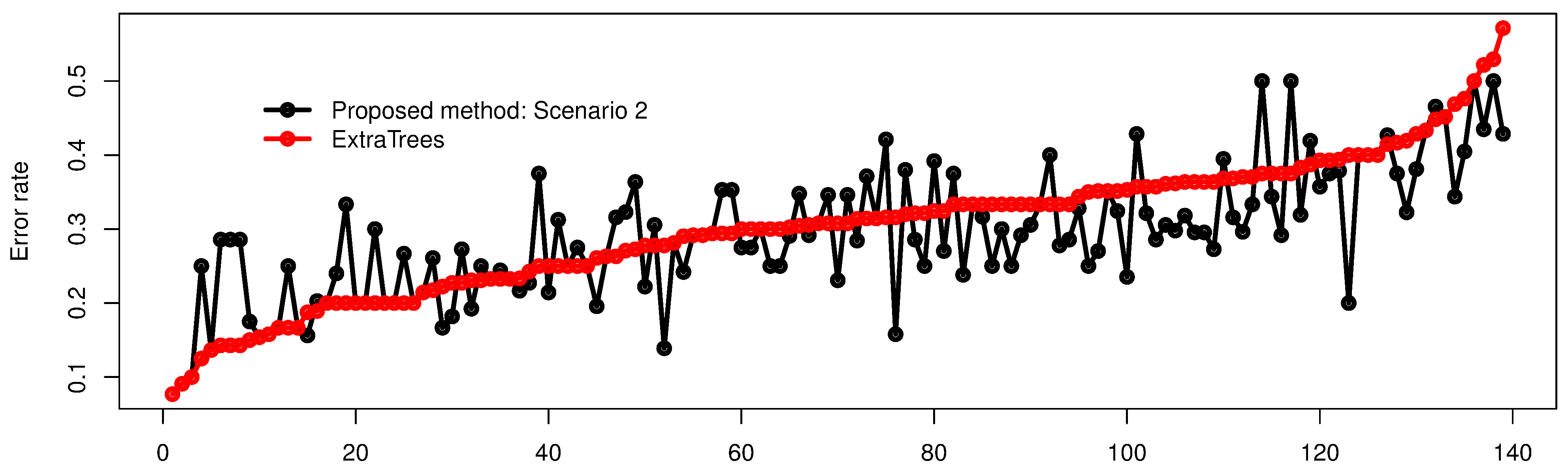
The proposed method with ${\lambda }_{k,j}$ determined by Scenario 2.

C:

AdaBoost trained with an individual dataset.

D:

AdaBoost trained with all datasets simultaneously.

We utilized $80\%$ of the training dataset for training of classifiers and the remaining $20\%$ for the validation. We repeated the above procedure 20 times and observed the averaged performance of the methods.

5.1.1. Dataset 1

We set the number J of tasks to three and assume that a marginal distribution of x is a uniform distribution on ${[-1,1]}^2$, and a discriminant function $F_j$ ($j=1,2,3$) associated with each dataset is generated by $F_j\left(x\right)=(1+c_{j,2})(x_1-c_{j,1})-x_2$, where $c_{j,1}\sim \mathrm{𝒩}(0,0.2^2)$ and $c_{j,2}\sim \mathrm{𝒩}(0,0.1^2)$. In addition, we randomly added a contamination noise on label y. Under these settings, we generated a training dataset, including 400 examples, and a test dataset, including 600 examples. Generated datasets are shown in Figure 2. We observe that each discriminant function and noise structure are different from the other two.

Figure 2. The three generated datasets and decision boundaries.

Figure 2. The three generated datasets and decision boundaries.

Figure 3 shows boxplots of the test errors of each method for datasets ${\mathrm{𝒟}}_j$ ($j=1,2,3$). We observe that the proposed method consistently outperforms individually trained AdaBoost, and AdaBoost trained with all datasets simultaneously. The figure shows that the proposed method can incorporate shared information among datasets into classifiers.

Figure 3. Boxplots of the test error of each method: A—proposed method with λ in Scenario 1; B—proposed method with λ in Scenario 2; C—AdaBoost trained with the individual dataset; D—AdaBoost trained with all datasets simultaneously; for three datasets, over the 20 simulation trials.

Figure 3. Boxplots of the test error of each method: A—proposed method with λ in Scenario 1; B—proposed method with λ in Scenario 2; C—AdaBoost trained with the individual dataset; D—AdaBoost trained with all datasets simultaneously; for three datasets, over the 20 simulation trials.

5.1.2. Dataset 2

We set the number J of tasks to 6 and assume that a marginal distribution of x is a uniform distribution on ${[-1,1]}^2$. Discriminant functions associated with each dataset are generated by:

$$\begin{array}{c}\hfill F_j\left(x\right)=\left\{\begin{array}{cc}(1+c_{j,2})(x_1-c_{j,1})-x_2,\hfill & j=1,2,3,\hfill \\ -(1+c_{j,2})(x_1-c_{j,1})+x_2,\hfill & j=4,5,6,\hfill \end{array}\right.\end{array}$$

where $c_{j,1}\sim \mathrm{𝒩}(0,0.1^2)$ and $c_{j,2}\sim \mathrm{𝒩}(0,0.1^2)$. In addition, we randomly added a contamination noise on label y. Under these settings, we generated training dataset, including 400 examples, and the test dataset, including 600 examples. Generated datasets are shown in Figure 4. We observe that Datasets 1, 2 and 3 share a structure, and Datasets 4, 5 and 6 share another structure.

Figure 4. The six generated datasets and decision boundaries.

Figure 4. The six generated datasets and decision boundaries.

Figure 5 shows boxplots of the test errors of each method for datasets ${\mathrm{𝒟}}_j$ ($j=1,...,6$). We omitted the result of AdaBoost trained with all datasets simultaneously (D) from the figure, because its performance is significantly worse than those of the other methods: the median of classification errors is around $0.5$. This is because the structures of Datasets 1, 2, 3 and Datasets 4, 5, 6 are opposite, and the labeling of concatenated dataset seems to be random. We observe that the proposed method with Scenario 2 (B) improves performance against individually-trained AdaBoost (C) and the proposed method in Scenario 1 (A). This is because the structure shared among Datasets 1, 2 and 3 does not have information about Datasets 4, 5 and 6 (and vice versa), and Method (B) can ignore the influence of the irrelevant information by adjusting ${\lambda }_{k,j}$ responding to $IS(q_{{\widehat{F}}_j},q_{{\widehat{F}}_k};r_k)$. Note that the performance of Method (A) is not so degraded, because the regularization parameter ${\lambda }_{k,j}$ was determined, so as to be zero, implying AdaBoost trained with the individual dataset.

Figure 6 shows examples of classification boundaries estimated by Methods A, B, C and D, for Dataset 6.

Figure 5. Boxplots of the test error of each method: A, Proposed method with λ in Scenario 1; B, proposed method with λ in Scenario 2; C, AdaBoost trained with the individual dataset ; for 6 datasets, over the 20 simulation trials.

Figure 5. Boxplots of the test error of each method: A, Proposed method with λ in Scenario 1; B, proposed method with λ in Scenario 2; C, AdaBoost trained with the individual dataset ; for 6 datasets, over the 20 simulation trials.

Figure 6. Classification boundaries by Methods A, B, C and D for Dataset 6. The blue line is the true classification boundary, and the red line represents the estimated classification boundary.

Figure 6. Classification boundaries by Methods A, B, C and D for Dataset 6. The blue line is the true classification boundary, and the red line represents the estimated classification boundary.

5.2. Real Dataset: School Dataset

In this section, we compared the proposed method (Scenario 2) to the a binary decision tree-based ensemble method, called extremely randomized trees (ExtraTrees) [23], applying to a real dataset, “school data”, reported from the Inner London Education Authority [24]. The dataset consists of examination records of 15,362 students from 139 secondary schools, i.e., we had 139 tasks. The dimension of input x is 27, in which original variables that are categorical were transformed into dummy variables. The original target variable $y_0$ represents score values in the range $[1,70]$, and we transformed the target variable $y_0$ to a binary variable as:

$$y=sgn(y_0-20).$$

We set the threshold to 20 to balance the ratio of classes ($-1:+1=7930:7432$). We randomly divided the dataset of each tasks into $80\%$ of the training dataset and remaining $20\%$ test dataset. In addition, we used $20\%$ of the divided training dataset as a validation dataset to determine the hyper-parameter λ and step number T. We repeated the above procedure 20 times and observed the average performance of the methods. Figure 7 shows the medians of error rates over 20 trials, by the proposed method and the ExtraTrees for 139 tasks. The horizontal axis indicates an index of a task, which is ranked in increasing order of the median error rate of the ExtraTrees. We observe that the proposed method is comparable to the ExtraTrees and especially has an advantage for tasks, in which the error rates of the ExtraTrees are large.

Figure 7. Medians of error rates by the proposed method and extremely randomized trees (ExtraTrees) for 139 tasks. The horizontal axis represents an index of a task, and the vertical axis indicates the median of error rates over 20 trials. Tasks are ranked in increasing order of the median error rate of the ExtraTrees.

Figure 7. Medians of error rates by the proposed method and extremely randomized trees (ExtraTrees) for 139 tasks. The horizontal axis represents an index of a task, and the vertical axis indicates the median of error rates over 20 trials. Tasks are ranked in increasing order of the median error rate of the ExtraTrees.

6. Conclusions

In this paper, we investigate the properties of binary classification with the pseudo model and reveal that minimization of the Itakura–Saito distance between the empirical distribution and the pseudo model is equivalent to AdaBoost and provides suitable properties for the binary classification. In addition, we pointed out that the Itakura–Saito distance is a unique divergence, having a suitable property for estimation with the pseudo model in the framework of the Bregman divergence. Based on the framework, we proposed a novel binary classification method for the multi-task learning, which incorporates shared information among tasks into the targeted task. The risk function of the proposed method is defined by the mixture of IS distance. The IS distance between pseudo models can be interpreted as the regularization term, incorporating shared information among tasks into the binary classifier for the target task. We investigated statistical properties of the risk function and derived computationally-feasible boosting-based algorithms. Furthermore, we considered a mechanism for the adjustment of the degree of information sharing and numerically investigated the validity of the proposed methods.

References

- Caruana, R. Multitask learning. Mach. Learn. 1997, 28, 41–75. [Google Scholar] [CrossRef]
- Pan, S.J.; Yang, Q. A survey on transfer learning. IEEE Trans. Knowl. Data Eng. 2010, 22, 1345–1359. [Google Scholar] [CrossRef]
- Argyriou, A.; Pontil, M.; Ying, Y.; Micchelli, C.A. A spectral regularization framework for multi-task structure learning. In Advances in Neural Information Processing Systems 19; MIT Press: Cambridge, MA, USA, 2007. [Google Scholar]
- Evgeniou, A.; Pontil, M. Multi-task feature learning. In Advances in Neural Information Processing Systems 19; MIT Press: Cambridge, MA, USA, 2007. [Google Scholar]
- Dai, W.; Yang, Q.; Xue, G.R.; Yu, Y. Boosting for transfer learning. In Proceedings of the 24th International Conference on Machine Learning, Corvallis, OR, USA, 20–24 June 2007; pp. 193–200.
- Wang, X.; Zhang, C.; Zhang, Z. Boosted multi-task learning for face verification with applications to web image and video search. In Proceedings of the IEEE Conference on Computer Vision and Pattern Recognition, Miami, FL, USA, 20–25 June 2009; pp. 142–149.
- Chapelle, O.; Shivaswamy, P.; Vadrevu, S.; Weiinberger, K.; Zhang, Y.; Tseng, B. Multi-task learning for boosting with application to web search ranking. In Proceedings of the 16th ACM SIGKDD International Conference on Knowledge Discovery and Data Mining, Washington, DC, USA, 25–28 July 2010; pp. 1189–1198.
- Cichocki, A.; Amari, S. Families of alpha- beta- and gamma-divergences: Flexible and robust measures of similarities. Entropy 2010, 12, 1532–1568. [Google Scholar] [CrossRef]
- Févotte, C.; Bertin, N.; Durrieu, J.L. Nonnegative matrix factorization with the Itakura–Saito divergence: With application to music analysis. Neural Comput. 2009, 21, 793–830. [Google Scholar] [CrossRef] [PubMed]
- Lefevre, A.; Bach, F.; Févotte, C. Itakura–Saito nonnegative matrix factorization with group sparsity. In Proceedings of the IEEE International Conference on Acoustics, Speech and Signal Processing (ICASSP), Prague, Czech, 22–27 May 2011; pp. 21–24.
- Takenouchi, T.; Komori, O.; Eguchi, S. A novel boosting algorithm for multi-task learning based on the Itakura–Saito divergence. In Proceedings of the Bayesian Inference and Maximum Entropy Methods in Science and Engineering (MaxEnt 2014), Amboise, France, 21–26 September 2014; pp. 230–237.
- Murata, N.; Takenouchi, T.; Kanamori, T.; Eguchi, S. Information geometry of U-boost and Bregman divergence. Neural Comput. 2004, 16, 1437–1481. [Google Scholar] [CrossRef] [PubMed]
- Banerjee, A.; Merugu, S.; Dhillon, I.S.; Ghosh, J. Clustering with Bregman divergences. J. Mach. Learn. Res. 2005, 6, 1705–1749. [Google Scholar]
- Amari, S.; Nagaoka, H. Methods of Information Geometry of Translations of Mathematical Monographs; Oxford University Press: Providence, RI, USA, 2000; Volume 191. [Google Scholar]
- Mihoko, M.; Eguchi, S. Robust blind source separation by beta divergence. Neural Comput. 2002, 14, 1859–1886. [Google Scholar] [CrossRef] [PubMed]
- Cichocki, A.; Cruces, S.; Amari, S.I. Generalized alpha-beta divergences and their application to robust nonnegative matrix factorization. Entropy 2011, 13, 134–170. [Google Scholar] [CrossRef]
- Takenouchi, T.; Eguchi, S. Robustifying AdaBoost by adding the naive error rate. Neural Comput. 2004, 16, 767–787. [Google Scholar] [CrossRef] [PubMed]
- Takenouchi, T.; Eguchi, S.; Murata, T.; Kanamori, T. Robust boosting algorithm against mislabeling in multi-class problems. Neural Comput. 2008, 20, 1596–1630. [Google Scholar] [CrossRef] [PubMed]
- Lafferty, G.L.J. Boosting and maximum likelihood for exponential models. In Advances in Neural Information Processing Systems 14; MIT Press: Cambridge, MA, USA, 2002. [Google Scholar]
- Evgeniou, T.; Pontil, M. Regularized multi-task learning. In Proceedings of the Tenth ACM SIGKDD International Conference on Knowledge Discovery and Data Mining, Seattle, WA, USA, 22–25 August 2004; pp. 109–117.
- Xue, Y.; Liao, X.; Carin, L.; Krishnapuram, B. Multi-task learning for classification with Dirichlet process priors. J. Mach. Learn. Res. 2007, 8, 35–63. [Google Scholar]
- Mason, L.; Baxter, J.; Bartlett, P.; Frean, M. Boosting algorithms as gradient decent in function space. In Advances in Neural Information Processing Systems 11; MIT Press: Cambridge, MA, USA, 1999. [Google Scholar]
- Geurts, P.; Ernst, D.; Wehenkel, L. Extremely randomized trees. Mach. Learn. 2006, 63, 3–42. [Google Scholar] [CrossRef]
- Goldstein, H. Multilevel modelling of survey data. J. R. Stat. Soc. Ser. D 1991, 40, 235–244. [Google Scholar] [CrossRef]
© 2015 by the authors; licensee MDPI, Basel, Switzerland. This article is an open access article distributed under the terms and conditions of the Creative Commons Attribution license (http://creativecommons.org/licenses/by/4.0/).
Share and Cite
Takenouchi, T.; Komori, O.; Eguchi, S. Binary Classification with a Pseudo Exponential Model and Its Application for Multi-Task Learning. Entropy 2015, 17, 5673-5694. https://doi.org/10.3390/e17085673
Takenouchi T, Komori O, Eguchi S. Binary Classification with a Pseudo Exponential Model and Its Application for Multi-Task Learning. Entropy. 2015; 17(8):5673-5694. https://doi.org/10.3390/e17085673
Chicago/Turabian StyleTakenouchi, Takashi, Osamu Komori, and Shinto Eguchi. 2015. "Binary Classification with a Pseudo Exponential Model and Its Application for Multi-Task Learning" Entropy 17, no. 8: 5673-5694. https://doi.org/10.3390/e17085673