Article

Computing and Learning Year-Round Daily Patterns of Hourly Wind Speed and Direction and Their Global Associations with Meteorological Factors

1
Institute of Ocean Technology and Marine Affairs, NCKU, No.1, University Road, Tainan, 70101,Taiwan
2
Department of Statistics, University of California, Davis, One Shields Avenue, 95616, CA, USA
*
Author to whom correspondence should be addressed.
Entropy 2015, 17(8), 5784-5798; https://doi.org/10.3390/e17085784
Submission received: 12 March 2015 / Revised: 16 June 2015 / Accepted: 3 August 2015 / Published: 11 August 2015
(This article belongs to the Special Issue Dynamical Equations and Causal Structures from Observations)

Abstract

:
Daily wind patterns and their relational associations with other metocean (oceanographic and meteorological) variables were algorithmically computed and extracted from a year-long wind and weather dataset, which was collected hourly from an ocean buoy located in the Penghu archipelago of Taiwan. The computational algorithm is called data cloud geometry (DCG). This DCG algorithm is a clustering-based nonparametric learning approach that was constructed and developed implicitly based on various entropy concepts. Regarding the bivariate aspect of wind speed and wind direction, the resulting multiscale clustering hierarchy revealed well-known wind characteristics of year-round pattern cycles pertaining to the particular geographic location of the buoy. A wind pattern due to a set of extreme weather days was also identified. Moreover, in terms of the relational aspect of wind and other weather variables, causal patterns were revealed through applying the DCG algorithm alternatively on the row and column axes of a data matrix by iteratively adapting distance measures to computed DCG tree structures. This adaptation technically constructed and integrated a multiscale, two-sample testing into the distance measure. These computed wind patterns and pattern-based causal relationships are useful for both general sailing and competition planning.

1. Introduction

As the world economy becomes more developed, many nations with ocean access are increasingly promoting sailing as a sport and as a leisure activity. Consequently, oceanic data collection and analysis have become vital parts of sailing promotion plans [1,2]. Thus, offshore ocean buoys have gradually assumed a new role beyond their traditional use for weather forecasting. The sampling rate of data-collecting devices mounted on ocean buoys is now being tuned to hourly or even sub-hourly. Across a wide range of variables, such frequently-collected data immediately face computing and analysis issues involving high dimensionality. Classic statistical techniques, such as regression or time series analyses, among others, are still hindered by unknown dependence structures embedded with multidimensional variables, even after applying dimensional reduction methodologies.
As a result, new computational methodologies are needed to extract proper information for making timely decisions. In this paper, we demonstrate that algorithmic computations can extract potentially useful pattern information for sailing competitions. From an organizer’s perspective, the region or location cannot be changed after the regatta venue has been determined. Furthermore, according to the policy of the International Sailing Federation (ISAF) [3], a race cannot be started if the wind speed falls below or exceeds the lower and upper limits, respectively, or if an expected or unexpected wind direction change occurs that is larger than a threshold value. Moreover, a race course is prepared a few hours ahead of a scheduled race based on the projected wind direction. Therefore, pattern information for daily wind speed and wind direction is required. Additionally, from the competitor’s perspective, a reliable prediction of hourly trajectories of wind speed and wind direction is very crucial [4]. Consequently, two scale-dependent pattern predictions are needed: (1) daily scale: the daily pattern of wind speed and wind direction based on all daily meteorological factors; and (2) hourly scale: to predict the hourly trajectory given the available hourly data before the target hour and daily data before the target day. In this paper, we first consider the daily scale goal and leave the hourly scale goal for future study. Our focal ocean buoy is located near Penghu, which is an archipelago under the jurisdiction of Taiwan located in the Taiwan Straits between Taiwan and China. Recordings are transmitted to the Center Weather Bureau of Taiwan on a round-the-clock basis. Note that an ocean buoy is subjected to daily weather trends, which are outlined as follows. Within a 24-hour period, a circular rhythmic pattern of wind direction occurs, which is attributed to the fact that the land is heated by the sun more quickly than is the sea. Therefore, the land generally has a higher temperature and lower air pressure than the sea surface during the day. This phenomenon creates sea breezes that peak in the early afternoon. In contrast, during the night, these temperature and air pressure factors reverse, which means that the land breezes peak at two or three hours after midnight. Accordingly, this cycle has two transitions around the ninth and 21st hours of a day. This cyclic effect is expected to be stronger for buoys located closer to islands and less evident for those located farther away. Such a sea-land breeze is a small-scale local phenomenon. Penghu also annually experiences a large-scale global monsoon effect, because the Sun heats different locations on the Earth heterogeneously across different seasons.
Moreover, the key meteorological factors collected include the following: (1) wind speed, (2) wind direction, (3) air temperature, (4) sea temperature, (5) air pressure and (6) wave height and wave period. For sailing purposes, the wind speed and wind direction are the two primary variables. In this paper, we compute and extract the year-round daily patterns from a bivariate dataset consisting of 339 daily 48( = 2 × 24 )-dimensional vectors from 2011. The 339 days, rather than 365 days, are the result of missing data from November. Then, we devote computing efforts to extracting potential causal linkages of other weather variables toward such computed patterns. Such patterns of wind speed and wind direction and their causal relationships with temperature and air pressure are potentially useful for the planning of sailing competitions.

2. Methods

2.1. Data and the Summarizing Minimum Ellipse

The 24-hour bivariate wind vectors are denoted as ( ν , θ ) in the polar coordinate system, with ν for wind speed and θ for wind direction. These vectors can be represented as a bivariate vector as ( ν cos θ , ν sin θ ) in a Cartesian coordinate system. That is, the magnitude of the vector is the wind speed, and the arrow points in the direction where the wind blows in the global coordinate system. As a daily example shown in Figure 1, the majority of the wind vector points are located in the 3rd quadrant, which indicates that the wind direction is primarily from south to southwest (a classic summer wind pattern).
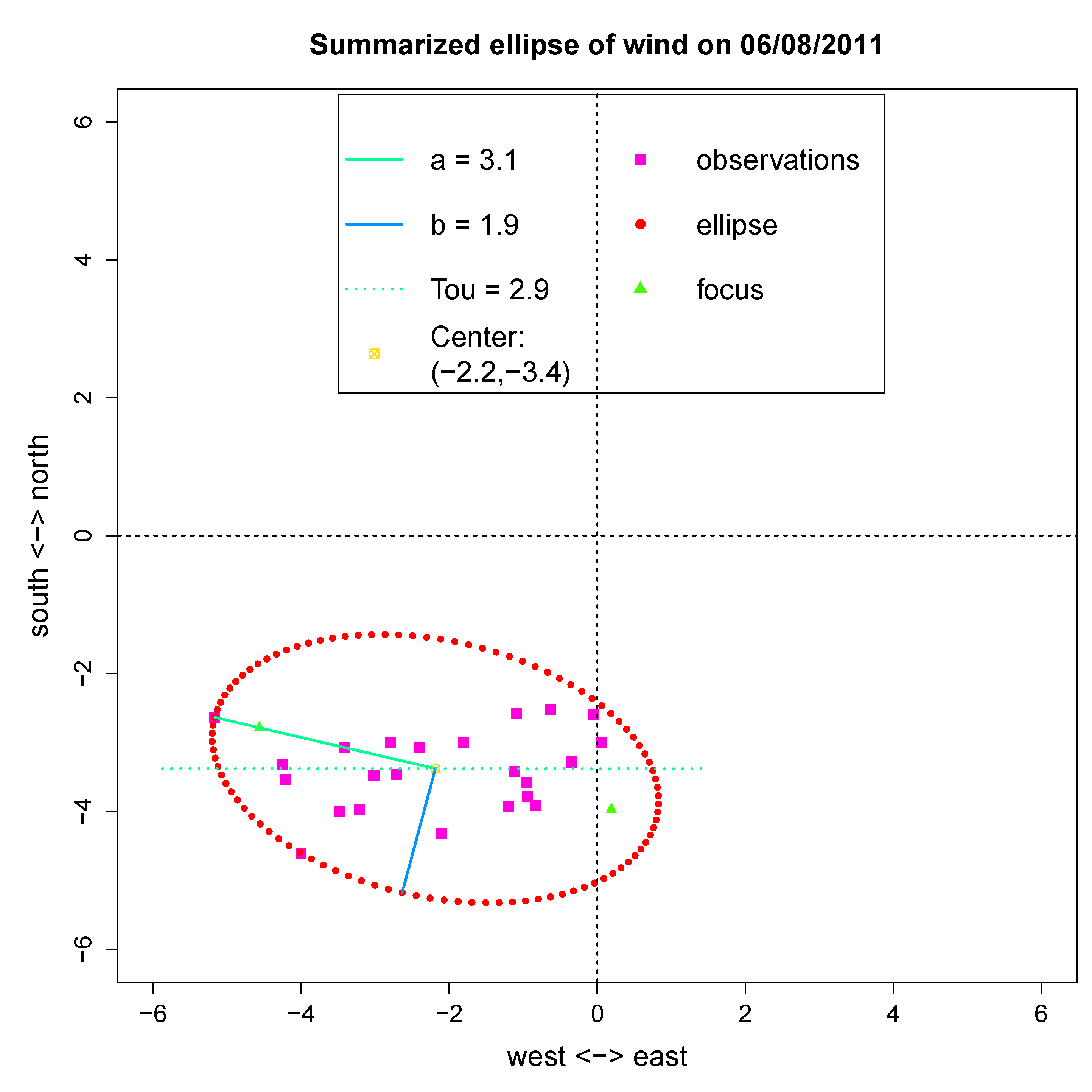
Figure 1. A summarizing ellipse constructed from daily wind speed and direction marked with the (1) 2-dimensional center of mass location, (2) lengths of the two axes and (3) tilt to the horizontal axis.
Entropy 17 05784 g001
Figure 2. 
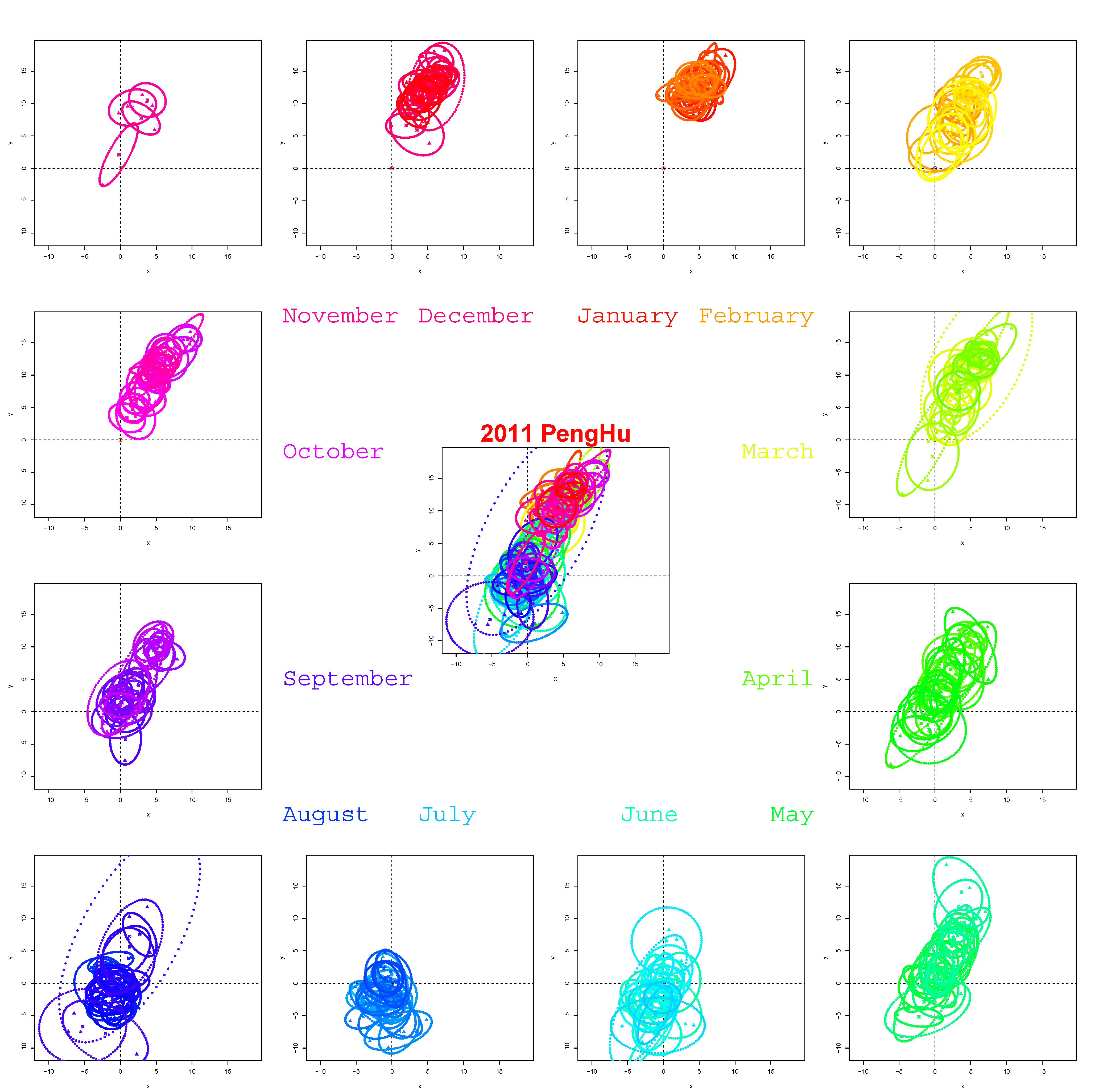
Three hundred thirty nine summarizing ellipses from 2011 displayed on 12 monthly panels.
Entropy 17 05784 g002
A summary statistic, called the minimum ellipse, is proposed to coherently capture the daily dynamic features of wind, as demonstrated by the ellipse shown in Figure 1. The minimum ellipse concept is based on the fact that the 24-hour wind speed and direction data indeed contain the aforementioned daily cycle [5]. The center of mass of such a point cloud relative to the origin of the coordinate system depicts the overall situation of the daily wind characteristics, which represents a large-scale weather pattern. When this center of mass falls within a small vicinity of the origin, the global geostrophic wind might be negligible, and the local daily cycle assumes the primary role in generating the wind pattern of the day. That is, when the point cloud coalesces around the origin with relatively large major axis lengths, it can be inferred that the wind direction changes along the major axes, which might be a land-sea breeze day. By contrast, when the point cloud is located far from the origin, the wind direction is more consistent. It is a day in which geostrophic wind dominates the wind pattern of the day. The average magnitude of wind speed depends on how far the center of mass is located from the origin. The directions of the major axis together with the directions of centers of mass determine the overall direction and direction changes. To compute the minimum ellipse, the following sequential steps are taken: (1) calculate the center of mass of 24 wind bivariate vectors; (2) identify the hourly wind vector that is located farthest away from the center of mass; draw a segment that links the center of mass and the farthest point, and take it as the major axis of the ellipse; (3) mark the angle of the segment of the major axis in the Cartesian coordinate system as the tilt of the ellipse; and (4) perform a recursive search via an ellipse constructed with a minor axis, such that all vectors are enclosed. The defining 5-dimensional parameters of such a computed ellipse include the following: the x and y-coordinates of its center of mass, the lengths of its major and minor axes and the angle of its major axis. The 5 ellipse parameters are given in the legend of Figure 1. The area of the ellipse represents the variation of the hourly wind vectors from the mean wind vector. They are not only informative, but also more appropriate than classic daily averages or maximums of wind speed or wind direction.
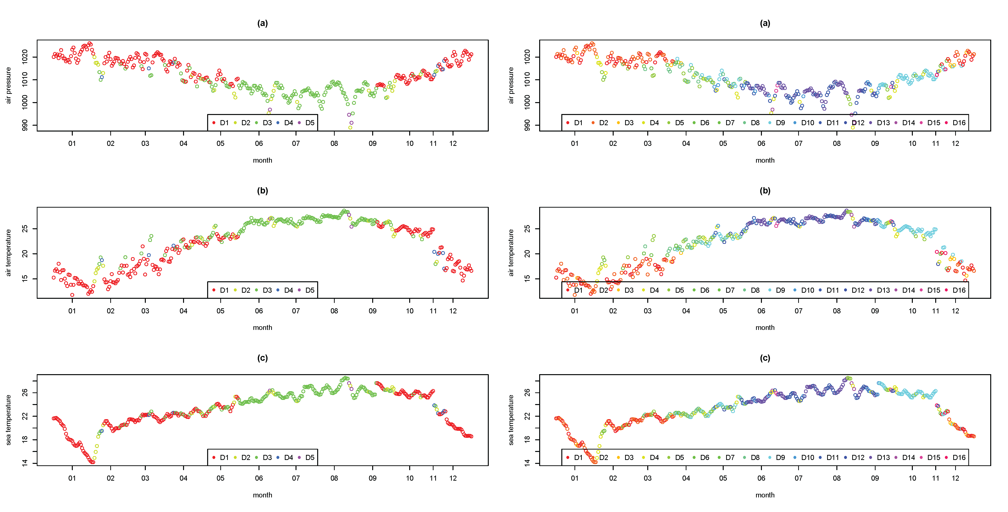
We now demonstrate that such 5-dimensional summary statistics are capable of revealing the informative and dynamic features of Penghu’s daily winds in 2011. The 339 daily summarized ellipses are grouped by month, with the entire year’s ellipses plotted at the center of Figure 2. This plot shows clear seasonal patterns with most of the ellipses in the upper panels located in the 1st quadrant, which represents the typical north-east monsoon in Penghu. Furthermore, ellipses in the lower panels are observed to move toward the origin. The ellipses moving toward the south-west indicate the classic summer wind patterns. In summary, the dynamic visible features include the following: (1) an evolving trajectory of extreme weather conditions, such as a typhoon’s approach and departure; (2) a new criterion for classifying daytime sea-land breezes; and (3) the yearly cycle of the characteristic northeast (NE)-monsoon.

2.1.1. Computations and Algorithms

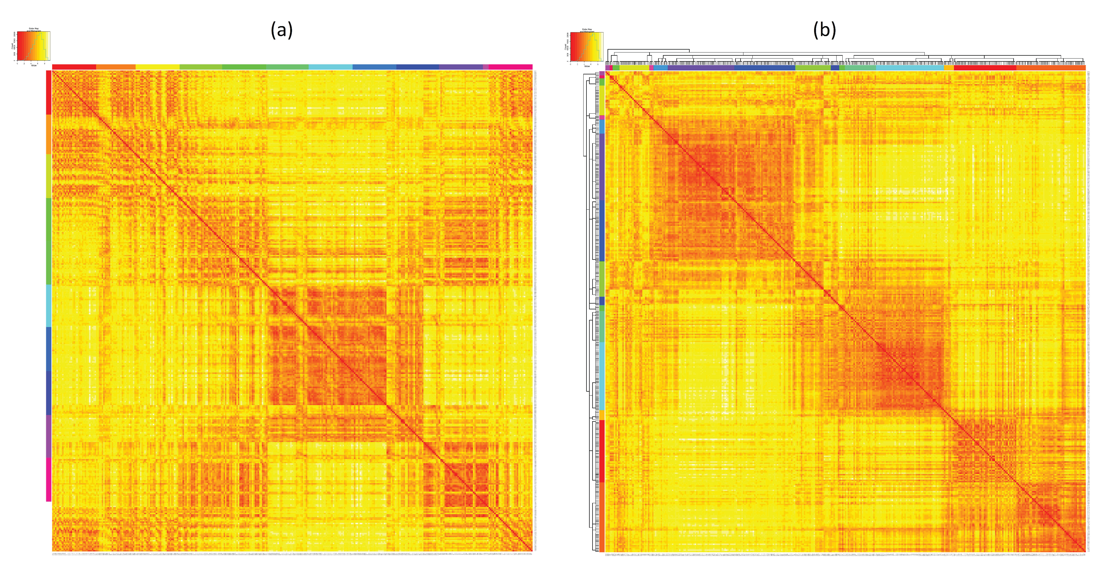
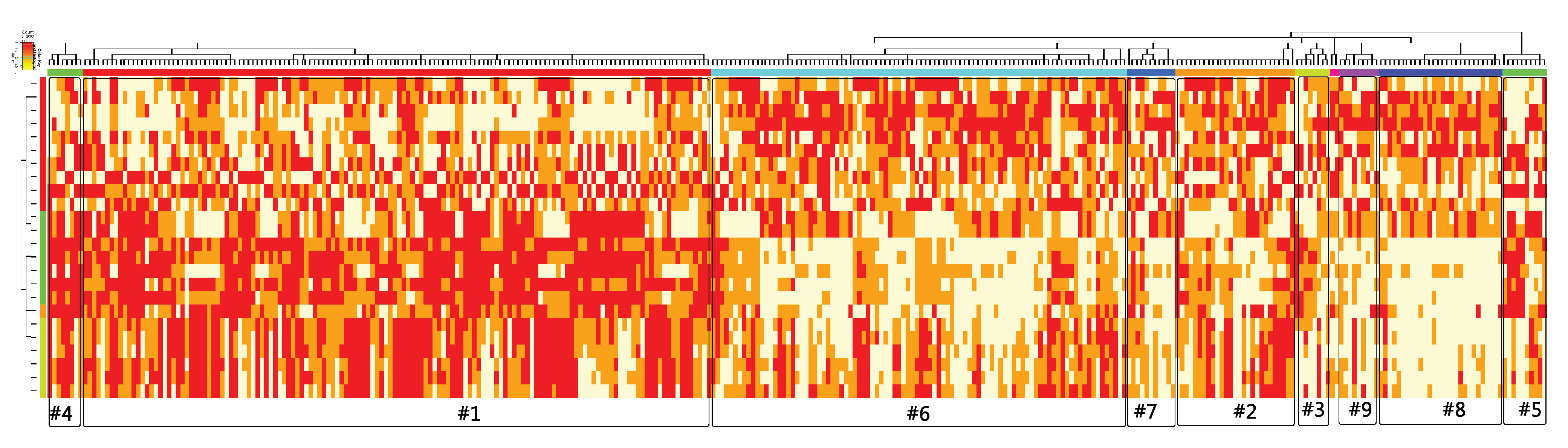
The major computational tool is the algorithm, called data cloud geometry (DCG), which produces an ultrametric DCG tree; see Fushing and McAssey (2010) [8] and Fushing et al. (2013) [9]. This DCG tree provides a multiscale clustering configuration on a node space, X = { x 1 , . . . . , x n } , in which an empirical measure of distance, d ( . , . ) , is typically derived from knowledge of the subject matter. With this distance measure, an n × n distance matrix is calculated and denoted as D [ X ] = [ d i j ] , with d i j = d ( x i , x j ) and i , j = 1 , . . . , n . Rather than directly using the matrix D [ X ] to arrive at a tree hierarchy of clustering, such as via the hierarchical clustering (HC) algorithm, the DCG algorithm works with a series of similarity matrices S ( T ) [ X ] = [ e - d i j / T ] indexed by scalar values T R + . The scale-tuning parameter T is specifically called “temperature” because of its statistical mechanics foundation. The concept and function of a temperature (scale) in DCG computing are similar to the concept and function of the “resolution” of a microscope. Under different resolutions, we observe distinct cell structures through a microscope instrument. Similarly, we expect the data to reveal distinct structural pattern information with respect to different temperatures. This temperature-regulated similarity matrix S ( T ) [ X ] is very distinct from the “time”-regulated device used in a diffusion map; see Coifman and Lafon (2006) [6].
Based on S ( T ) [ X ] , a trajectory ensemble of node removal-regulated Markov random walks is generated. The random walk, which is defined through a transition probability matrix converted from S ( T ) [ X ] , is a tool for determining the temperature-specific data geometry. To be able to explore the whole landscape without being trapped within a cluster, the design of such a random walk is to remove a node after it has been visited over a threshold number of visits. Thus, with the random traveling among nodes, the number of nodes becomes increasingly smaller. When a random walk explores a landscape of nodes, we also count the number of steps required to remove the next node. A larger number of steps is typically required to remove the first node when it enters into a new cluster. This feature of node removal produces spikes on the node-removal recurrence time process. Thus, a spike indicates that a random walk enters a newly unexplored cluster. Therefore, two pieces of information become available on a node removal recurrence time process: (1) the number of spikes indicates the number of clusters under the temperature T; and (2) all removed nodes between two successive spikes are likely to be located in the same cluster. Consequently, a node removal-regulated random walk gives rise to a binary connectivity matrix with 1 or 0 at the ( i , j ) entry according to whether nodes x i and x j are removed between the same pair of successive spikes. An ensemble of random walks gives rise to an ensemble of binary-connected matrices. By averaging such an ensemble of binary-connected matrices, a connectivity or cluster-sharing probability matrix can be obtained. From this connectivity probability matrix, the clustering configuration pertaining to the temperature T can be extracted. Finally, a subset of temperatures is selected, each of which provides confidence in the extracted temperature-specific clustering configuration. Then, an ultrametric tree algorithm is applied (see Fushing et al. (2013) [9] for the detailed construction), for which the Ultrametric DCG-tree on χ is denoted as T [ X ] .
For example, 𝒳 is the space of 339 ( = n ) daily 5-dimensional summarizing parameters of an ellipse for 2011. d ( x i , x j ) is the weighted Euclidean distance of R 5 with weighted proportional standard deviations of the 5 dimensions. A daily wind ultrametric tree 𝒯 [ X ] 
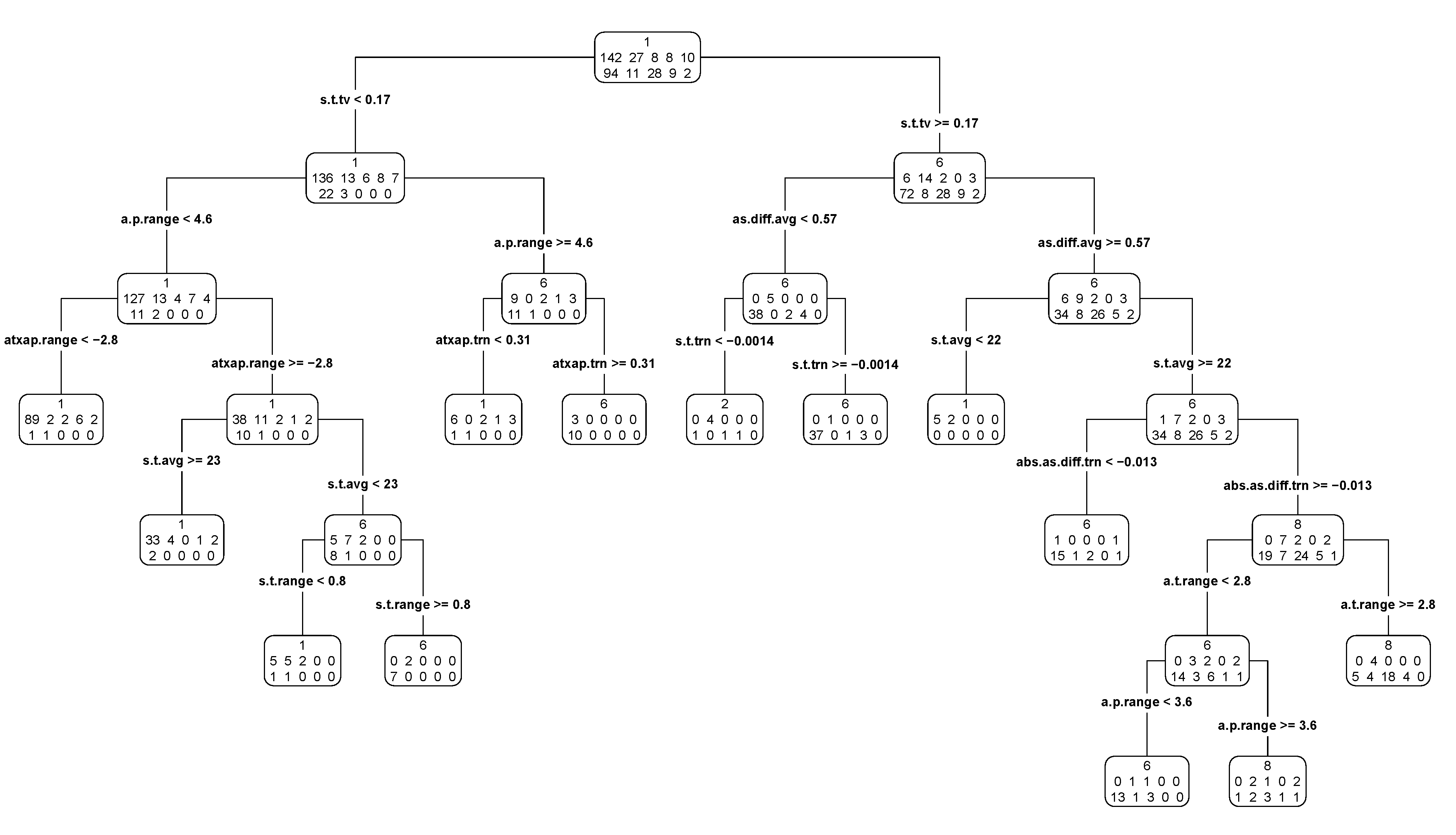
can then be computed, as presented in the subsequent section. Next, we discuss an algorithm for adapting the Euclidean distance to an ultrametric tree structure. For example, consider the 339 × 24 covariate matrix. Let the node space on the column axis be denoted as Y = { y 1 , . . . . , y 24 } . Therefore, y j is a R 339 vector for each j = 1 , . . , 24 . Then, a new Euclidean distance is defined by adapting the chosen T [ X ] tree structure on the 339 day nodes. Each covariate is represented by a 339-dimensional vector. On Level 0, the Euclidean distance is computed by summing 339 component-wise discrepancies between two covariate vectors. One level up, for instance, supposes that there exists a known 10-cluster structure among 339 daily nodes. Upon this 10-cluster structure, we can further manifest the degree of discrepancy/concordance between any pair of covariates by separating the 339 dimensions into 10 categories and evaluating their discrepancy/concordance upon the corresponding 10 dimensions. The evaluation involves calculating the difference in pairwise averages within each category and summing them. That is, to a great extent, we accommodate 10 two-sample testing statistics into our new distance measurement. The algorithm is described as follows. Any level of the tree T [ X ] corresponds to a clustering composition of χ. Suppose that L X ( 1 ) levels (including the bottom level) of the tree are chosen to form a multiscale collection of clusters on χ. This collection is denoted as { C X ( 1 ) ( l , h ) | l = 1 , . . , L X ( 1 ) 1 ; h = 1 , . . . , H ( l ) X } , where H ( l ) X is the number of clusters C X ( 1 ) ( l , h ) on the l-th level. Each cluster size is denoted as | C X ( 1 ) ( l , h ) | . The updated distance d Y ( 1 ) from the Euclidean distance d Y ( 0 ) on Y R m is defined as follows:
d Y ( 1 ) ( y i , y j ) = d Y ( 0 ) + { l = 1 L Y ( 1 ) h = 1 H ( l ) X | C X ( 1 ) ( l , h ) | [ μ ( y i | C X ( 1 ) ( l , h ) ) - μ ( y j | C X ( 1 ) ( l , h ) ) ] 2 } 1 / 2 ,
where d Y ( 0 ) is the Euclidean distance and μ ( y i | C X ( 1 ) ( l , h ) ) is the average of components y i ( R m ) in C X ( 1 ) ( l , h ) , which is μ ( y j | C X ( 1 ) ( l , h ) ) for y j .
This adaptation algorithm comprises the heart of the computational algorithm and is called data mechanics (DM) in Fushing et al. (2014) [7]. This algorithm is designed to extract interacting relational patterns between two node spaces, with data being represented as a rectangular matrix, such as the 339 × 24 covariate matrix. This data-driven distance indicates how to operationally couple tree-structural information from a given different node space to a target node space. Two vectors corresponding to two nodes, y i and y j , which have a relatively small Euclidean distance via d Y ( 0 ) , do not necessarily have a small distance via d Y ( 1 ) ( y i , y j ) . This discrepancy is due to the clustering configuration L X ( 1 ) ; hence, it becomes essential and critical for computing causal and predictive patterns.

3. Results and Discussion

In this section, our computational results are reported, followed by a comparison with a decision tree.

3.1. Multiscale Community Structures of Daily Wind

We now compute the Euclidean distance matrix of daily pairs of five-dimensional vectors, which are constructed from standardized summary ellipse parameters. A DCG tree of daily wind is created based on the distance matrix. This hierarchy tree contains five levels, which partition all days of the year into 2, 5, 10, 18 and 42 clusters. A symmetric heat map was created based on the distance matrix with both rows and columns arranged according to the DCG tree structure, as shown in Figure 3. This daily wind DCG tree embedded heat map clearly shows five- and 10-block diagonal structures. Five colors are assigned to the five clusters of the five-cluster level on the column axis; likewise, 10 colors are assigned to the 10-cluster level on the row axis of the daily wind DCG tree.
The five-cluster level separates days of the year into one major cluster of “typical” wind days, with the four remaining clusters as characteristically strong or extremely strong wind days. In particular, the cluster on the edge of the column axis contains extreme winds due to the strong typhoon “Nanmadol” that passed by Penghu on 29th–30th of August 2011. The obvious light color on the far right and bottom strips of the heat map shows that these days were very distinct from the other days of the year. In actuality, the daily wind DCG tree successfully captures the clustered minimum ellipses that represent these extreme weather days in cluster No. 5 of Figure 4 (10-cluster level).
To obtain further details, the contents of the daily ellipses on the 10-cluster level of the daily wind DCG tree are displayed in Figure 4. The two largest clusters (No. 1 and No. 6) represent the northeast monsoon in winter and the transition period from NE–SW monsoon. Cluster No. 8 contains the daily members between the months of April and September, which is the characteristic SW monsoon season. As shown, the ellipse shape and location of members in this particular cluster are rather uniform; by contrast, the days in cluster No. 2 are dispersed throughout the year. This is not an expected seasonal cluster, in which ellipses’ chain-overlapping connections are evident. Moreover, this cluster demonstrates the ability of a daily wind DCG tree to capture evolving patterns.
Figure 3. Heat map constructed from the daily wind data cloud geometry (DCG) tree.
Entropy 17 05784 g003
Figure 4. Ten summary ellipse clusters based on a DCG tree.
Entropy 17 05784 g004
We then take the computed multiscale patterns of wind speed and wind direction as patterns for response variables. The next task is to attempt to explain why such patterns arise. That is, we would like to determine whether other weather variables, such as air pressure, sea temperature and air temperature recorded by an ocean buoy, could provide insights into wind patterns. We also include the sea-to-air temperature difference and the product of air temperature and air pressure, because these parameters are theoretically correlated with wind patterns. We aggregate these covariates (by mean, range, linear trend and total variation) from hourly observations to construct 24-dimension daily weather covariates; see the Appendix for details. We discretely categorize each variable into three categories by their corresponding one-third and two-third quantiles. In this way, a 339 covariate matrix is derived; in other words, each covariate variable has 339 dimensions. A distance is devised for these 24 covariate vectors. By following the daily wind DCG tree on the 339 nodes, this distance becomes a three-level distance derived as in DM-Step 2 with Level 0 for the bottom level of 339 days, Level 1 for the 10-cluster level and Level-2 for five-cluster level.

3.2. Relationships between Daily Wind DCG Trees and Meteorological Covariates

A 24 × 24 distance matrix of these 24 covariates can now be generated, yielding a DCG tree constructed based on this distance matrix, as shown in Figure 5. Note that this covariate DCG tree is embedded with structural information of the daily wind DCG tree with respect to the 339 day nodes. The top covariate DCG tree level essentially separates the 24 covariates into one group associated with air pressure and another associated with temperature. As shown, the linear trend of sea temperature (s.t.trn) is singleton on the second level of the covariate DCG tree. This result is reasonable because sea temperature is affected not only by weather conditions, but also by ocean currents.
Figure 5. Twenty four covariate-factor DCG tree based on 339-dimdaily measurements with distance modified by the daily-wind DCG tree.
Entropy 17 05784 g005
Based on the three-level covariate DCG tree structure, we then similarly derive a new distance according to DM-Step 2 on the collection of 339 daily 24-dimensional vectors. A 339 × 339 distance matrix was thus calculated. A heat map version of this distance matrix with all rows and columns marked by month is presented in Figure 6a. It is evident that this heat map reveals clear cyclic patterns of seasonal blocks structured by month. Additionally, a new daily covariate DCG tree was constructed on the 339 day nodes based on this distance matrix. The color of a day in a month Figure 6b was kept the same as in (a). Accordingly, the monthly color segments are more or less intact. Only the winter months are merged against spring and fall months in this new daily covariate DCG tree. Another heat map version of the distance matrix with all rows and columns arranged according to this daily covariate DCG tree is presented in Figure 6b. Again, this heat map reveals evident block patterns that characterize the wind seasons of Penghu.
Figure 6. Heat maps of the daily covariate distance matrix. (a) The distance matrix ordered by date and (b) the distance matrix ordered by DCG tree.
Entropy 17 05784 g006
To further demonstrate that the daily covariate DCG tree successfully separates seasonal patterns, clusters were marked on the five-cluster level and 16-cluster level with color. The colored days are then displayed according to the calendar for three weather variables: (a) air pressure, (b) air temperature and (c) sea temperature, as in Figure 7. The resulting cyclic patterns can thus be observed. These plots illustrate that the daily covariate DCG tree has the ability to accurately capture the seasonal effects of this dynamic system.
In summary, it was demonstrated that the daily covariate DCG tree embedded with structural information from the daily wind DCG tree can indeed reveal seasonal weather patterns. These multiscale coherence results are interpreted as holistic indications that there exists the potential for mutual causal and predictable relationships between the covariate and daily wind DCG trees. The multiscale refers to the level-to-level correspondence. On each focal level, such causal and predictive interpretations further imply that collective clusters of daily 24-dimensional covariate variables and clusters of 48-dimensional wind speed and wind direction are mutually associated. These relationships can be visualized to a great extent in Figure 8.
Figure 7. Year-round series of three covariate variables: (a) air pressure, (b) air temperature and (c) sea temperature color marked on the five-cluster level (left panel) and 16-cluster level (right panel) of the DCG tree.
Entropy 17 05784 g007
Figure 8. Heat map of covariate matrix ordered by the 24-covariate DCG tree coupled with the daily wind DCG tree marked on the 10-cluster level.
Entropy 17 05784 g008

3.3. Comparisons with Decision Tree

In contrast to the above collective and holistic relationships, a decision tree provides many layers of one-variable-at-a-time relationships. Although decision trees have recently become a common method for classification problems, are such one-variable-at-a-time relationships valid in a system setting? The main driving force for this validity doubt is that all covariate variables are associated in unknown and nonlinear manners with heterogeneous degrees. It is also known that decision trees typically have high probabilities of overfitting [10]. However, we employ this potential overfitting property of a decision tree to compare the causal effects of our computed covariate DCG tree with the daily wind DCG tree. We use the 24 original covariates as a predictor to classify each day into one of the 10 clusters found in the daily wind DCG tree. This clustering configuration is used as a priori knowledge for constructing the decision tree, which resulted in a tree with 13 leaves. The chosen splitting variables selected by the recursive partition tree from the tree top are the “total variation of sea temperature”, followed by “daily range of air pressure” on the left side and “average air-sea temperature difference” on the right side, and the full decision tree is shown in Figure 9. The detailed bifurcations result in many multiple partitions on all 10 daily wind clusters. This phenomenon is ubiquitous over the entire decision tree, which is taken as evidence of misclassification. Note that the selected variables are difficult to match with the two major systemic wind patterns (winter vs. fall and spring) in Penghu. Additionally, the constant bifurcating split is not data driven and is thus somewhat artificial.
Figure 9. The decision tree classified the 10 daily wind clusters with the 24 original covariate variables.
Entropy 17 05784 g009
To express the causal effects of our computed covariate DCG tree on the daily wind DCG tree, the daily ellipse distance heat map was employed. The row axis of this distance matrix is arranged according to the daily wind DCG tree, while its column axis is arranged according to the daily covariate DCG tree, as shown in Figure 10a. The block structural patterns indicate the correspondences between clusters on the two coupled trees; in other words, collective causal relations are present. For the contrasting heat map presented in Figure 10b, the same distance matrix is used, with its column axis arranged with 13 respective leaves taken from the decision tree in Figure 9 [11]. The two heat maps exhibit rather similar structural block patterns. We conclude that the covariate DCG tree has at least the same casual effects as the decision tree. Note that the decision tree directly uses the 10 configuration information clusters from the daily wind DCG tree as a priori knowledge, whereas our computed covariate DCG tree indirectly uses the same information through distance adaptation.
Figure 10. The 339-by-339 heat map of daily ellipse distances with rows arranged according to the daily wind DCG tree and columns arranged according to the (a) covariate DCG tree and (b) the leaves of the fitted decision tree.
Entropy 17 05784 g010

4. Conclusions

In this article, we introduced the minimum ellipse method to summarize the hourly observed wind data in a day. A DCG tree was used to cluster the wind patterns within a year. From the results of the daily wind DCG tree, the meteorological covariate’s hierarchical structure could be obtained. We also demonstrated that the DCG tree successfully captured the seasonal pattern from the hourly observed meteorological covariates. By coupling the covariates’ DCG tree with the daily wind DCG tree, the causal effects could be observed within these two DCG tree structures. The proposed method performs well compared to the popular decision tree method, but avoids the potential overfitting issue.

Acknowledgments

This research was supported in part by the NSF under Grant No DMS 1007219 (co-funded by Cyber-enabled Discovery and Innovation (CDI) program) (H.F.). This study was also partially funded by the Graduate Students Study Abroad Program and research project NSC 102-2221-E-006-150 (Marine Weather Analysis for Recreational Boating Activity in the Dapeng Bay National Scenic Area) of the National Science Council of Taiwan (H.T.W. and L.Z.H.C.).

Author Contributions

Hsing-Ti Wu designed the study, analyzed and interpreted the data, produced the results and drafted the manuscript. Hsieh Fushing designed the study, interpreted the data and revised the article. Laurence Z.H. Chuang participated in the collection of data and interpreted the results. All authors have read and approved the final manuscript.

Appendix

There are three covariates observed hourly from the data buoy. Twenty four observations were collected hourly each day for each item. These covariates include sea level pressure (PRES), air temperature (ATMP) and sea surface temperature (WTMP). We derived another three variables from the original three observations, namely the difference between air and sea temperature, the absolute difference of air and sea temperature and the interaction term computed from the air pressure multiplied by air temperature. We then summarized these six characteristics with four types of summary statistics (mean, range, total variation and linear trend). Consequently, 24 covariates representing each day were produced. Afterward, we categorized the covariates by a one-third quantile. Finally, each covariate has a value of 1, 2 or 3, representing low, medium and high levels, respectively.
Let x = x 1 , x 2 , , x 24 be one of the six characteristics observed in a day. Then, the four statistics can be calculated as
mean: x ¯
range: m a x ( x ) - m i n ( x )
total variation: i = 1 23 | x i + 1 x i |
linear trend: regression coefficient a 1 with x t = a 0 + a 1 t (   t = 1 , , 24 )
The variable names of the final 24 covariates are listed in Table 1.
Table 1. List of covariate names.
Statistics
Observationsmeanrangetotal variationlinear trend
P R E S a.p.avga.p.rangea.p.tva.p.trn
A T M P a.t.avga.t.rangea.t.tva.t.trn
W T M P s.t.avgs.t.ranges.t.tvs.t.trn
A T M P - W T M P as.diff.avgas.diff.rangeas.diff.tvas.diff.trn
| A T M P - W T M P | abs.as.diff.avgabs.as.diff.rangeabs.as.diff.tvabs.as.diff.trn
P R E S × A T M P atxap.avgatxap.rangeatxap.tvatxap.trn

Conflicts of Interest

The authors declare no conflicts of interest.

References

  1. Dunsmuir, W.T.M.; Spark, E.; Kim, S.K.; Chen, S.L. Statistical prediction of sea breezes in Sydney Harbour. Aust. Meteorol. Mag. 2003, 52, 117–126. [Google Scholar]
  2. Ma, Y.; Gao, R.Z.; Xue, Y.C.; Yang, Y.Q.; Wang, X.Y.; Liu, B.; Xu, X.L.; Liu, X.Z.; Hou, J.W.; Lin, H. Weather Support for the 2008 Olympic and Paralympic Sailing Events. Adv. Meteorol. 2013, 2013. [Google Scholar] [CrossRef]
  3. International Sailing Federation. Race Management Policies for the Olympic Sailing Competition and ISAF Events; International Sailing Federation: Southampton, UK, 2011; pp. 1–11. [Google Scholar]
  4. Cort, A.; Stearns, R. Getting Started in Sailboat Racing; McGraw-Hill Education: New York, NY, USA, 2004. [Google Scholar]
  5. Breckling, J. The Analysis of Directional Time Series: Applications to Wind Speed and Direction; Springer: New York, NY, USA, 1989. [Google Scholar]
  6. Coifman, R.R.; Lafon, S. Diffusion maps. Appl. Comput. Harmonic Anal. 2006, 21, 5–30. [Google Scholar] [CrossRef]
  7. Fushing, H.; Chen, C. Data Mechanics and Coupling Geometry on Binary Bipartite Networks. PLoS One 2014, 9. [Google Scholar] [CrossRef] [PubMed]
  8. Fushing, H.; McAssey, M.P. Time, temperature, and data cloud geometry. Phys. Rev. E 2010, 82. [Google Scholar] [CrossRef]
  9. Fushing, H.; Wang, H.; VanderWaal, K.; McCowan, B.; Koehl, P. Multi-Scale Clustering by Building a Robust and Self Correcting Ultrametric Topology on Data Points. PLoS One 2013, 8. [Google Scholar] [CrossRef] [PubMed]
  10. Hothorn, T.; Hornik, K.; Zeileis, A. Unbiased recursive partitioning: A conditional inference framework. J. Comput. Graph. Stat. 2006, 15, 651–674. [Google Scholar] [CrossRef]
  11. Breiman, L.; Friedman, J.; Stone, C.J.; Olshen, R.A. Classification and Regression Trees; Taylor & Francis: Oxon, UK, 1984. [Google Scholar]

