
Bounds on Rényi and Shannon Entropies for Finite Mixtures of Multivariate Skew-Normal Distributions: Application to Swordfish (Xiphias gladius Linnaeus)


Abstract
:1. Introduction
2. Preliminary Material
2.1. Skew-Normal Distribution
2.2. Finite Mixtures of Skew-Normal Distributions
2.3. Entropies
- (i)
- the Shannon entropy of iswherewith .
- (ii)
- the αth-Rényi entropy of , , iswherewith , , , is the α-dimensional vector of ones, and .
3. Results
3.1. Shannon Entropy Bounds
- (i)
- ,
- (ii)
- ,
3.2. Rényi Entropy Bounds
4. Numerical Results
4.1. Simulations
4.2. Application
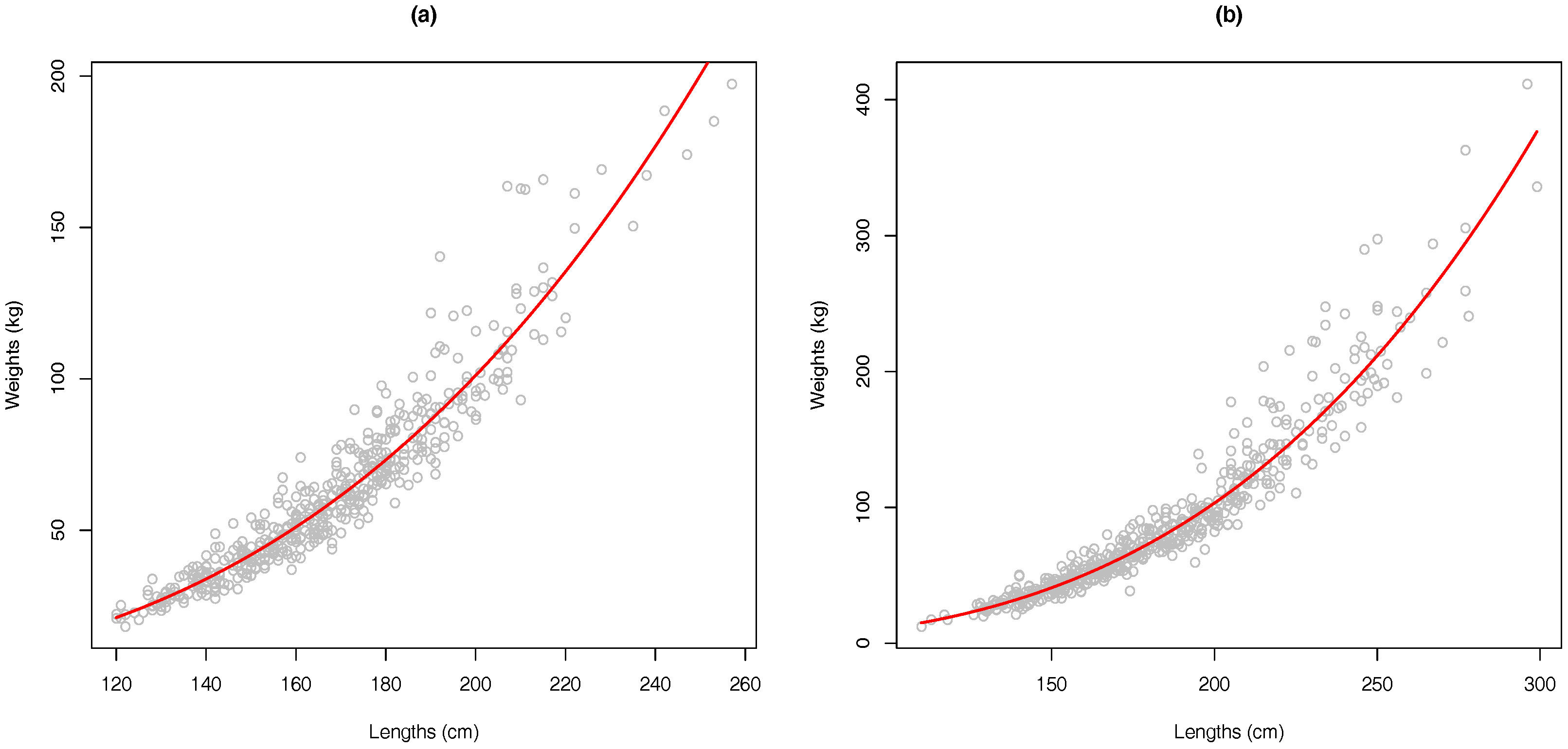
- (a)
- The matrix of data includes both length and weight () for each observation. Because it is necessary to avoid colinearity, the length–weight regression is computed to show non-linear relationship among both columns.
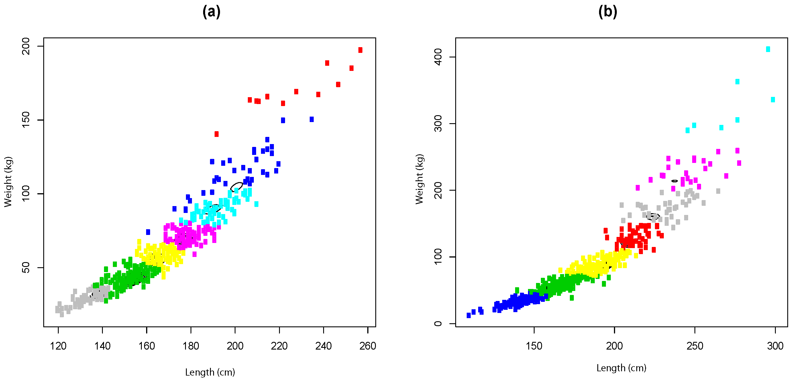
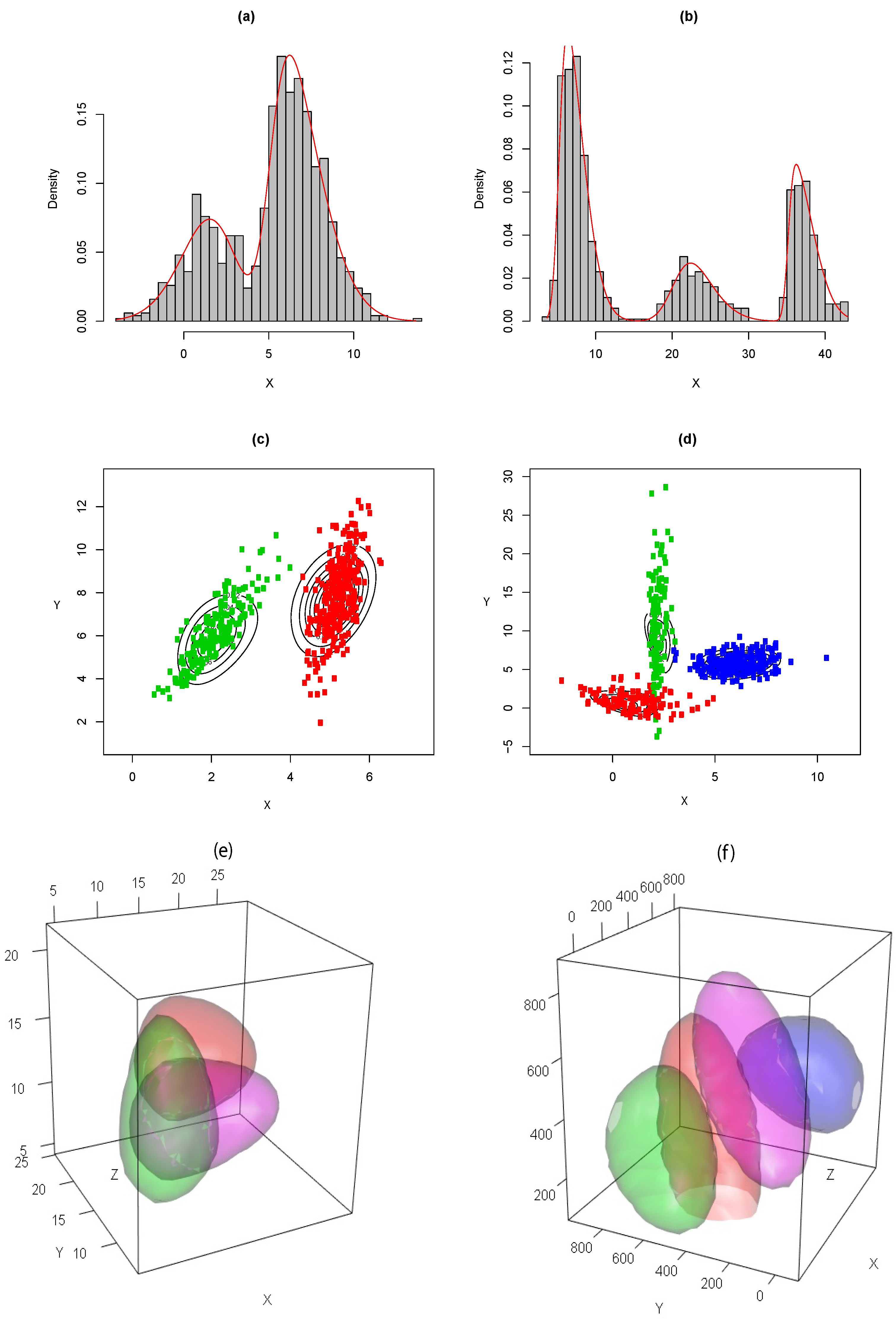
- (b)
- Given that the number of components is unknown (age is unknown), the FMSN parameters are estimated considering the two-dimensional matrix of the last step for several values m.
- (c)
- The number of components is determined by the bounds of information measures developed in Section 3 and then compared with AIC and BIC criteria.
- (d)
- The observed (measures obtained from the procedure of [30]) and estimated (by selected mixture model) ages of all observations are compared using a misclassification analysis.
4.2.1. Data and Software
4.2.2. Length–Weight Relationship
4.2.3. Clustering and Model Selection
5. Conclusions
5.1. Methodology
5.2. Application
Supplementary Materials
Acknowledgments
Author Contributions
Conflicts of Interest
Appendix A
- (i)
- For any finite mixture , where is the associated parameter set of each i-th component , , , , and is not necessarily normal with non-zero location vector and dispersion matrix Λ. Then,For a proof of Equation (A1), see pp. 27 and 663 of [20]. Basically, the fact that is a concave function ( is convex) allows the use of Jensen’s inequality. Then, considering the location vector (7) and dispersion matrix (8), we have the inequalities and . Considering the property (i) of Proposition 1 and the condition , we prove the left side of the inequality.
- (ii)
References
- McLachlan, G.; Peel, D. Finite Mixture Models; John Wiley Sons: New York, NY, USA, 2000. [Google Scholar]
- Celeux, G.; Soromenho, G. An entropy criterion for assessing the number of clusters in a mixture model. J. Classif. 1996, 13, 195–212. [Google Scholar] [CrossRef]
- Jenssen, R.; Hild, K.E.; Erdogmus, D.; Principe, J.C.; Eltoft, T. Clustering using Renyi’s entropy. IEEE Proc. Int. Jt. Conf. Neural Netw. 2003, 1, 523–528. [Google Scholar]
- Amoud, H.; Snoussi, H.; Hewson, D.; Doussot, M.; Duchêne, J. Intrinsic mode entropy for nonlinear discriminant analysis. IEEE Signal Process. Lett. 2007, 14, 297–300. [Google Scholar] [CrossRef]
- Caillol, H.; Pieczynski, W.; Hillion, A. Estimation of fuzzy Gaussian mixture and unsupervised statistical image segmentation. IEEE Trans. Image Process. 1997, 6, 425–440. [Google Scholar] [CrossRef] [PubMed]
- Carreira-Perpiñán, M.A. Mode-finding for mixtures of Gaussian distributions. IEEE Trans. Pattern Anal. Mach. Intell. 2000, 22, 1318–1323. [Google Scholar] [CrossRef]
- Durrieu, J.-L.; Thiran, J.; Kelly, F. Lower and upper bounds for approximation of the Kullback–Leibler divergence between Gaussian mixture models. In Proceedings of the 2012 IEEE International Conference on Acoustics, Speech and Signal Processing (ICASSP), Kyoto, Japan, 25–30 March 2012; pp. 4833–4836.
- Nielsen, F.; Sun, K. Guaranteed bounds on the Kullback–Leibler divergence of univariate mixtures. IEEE Signal Process. Lett. 2016, 23, 1543–1546. [Google Scholar] [CrossRef]
- Huber, M.F.; Bailey, T.; Durrant-Whyte, H.; Hanebeck, U.D. On entropy approximation for Gaussian mixture random vectors. In Proceedings of the IEEE International Conference on Multisensor Fusion and Integration for Intelligent Systems, Seoul, Korea, 20–22 August 2008; pp. 181–188.
- Rényi, A. On measures of entropy and information. In Proceedings of the Fourth Berkeley Symposium on Mathematical Statistics and Probability, Berkeley, CA, USA, 20 June–30 July 1960; Neyman, J., Ed.; University of California Press: Berkeley, CA, USA, 1961; Volume 1, pp. 547–561. [Google Scholar]
- Contreras-Reyes, J.E. Rényi entropy and complexity measure for skew-gaussian distributions and related families. Physica A 2015, 433, 84–91. [Google Scholar] [CrossRef]
- Zografos, K.; Nadarajah, S. Expressions for Rényi and Shannon entropies for multivariate distributions. Stat. Probab. Lett. 2005, 71, 71–84. [Google Scholar] [CrossRef]
- Lin, T.I. Maximum likelihood estimation for multivariate skew normal mixture models. J. Multivar. Anal. 2009, 100, 257–265. [Google Scholar] [CrossRef]
- Frühwirth-Schnatter, S.; Pyne, S. Bayesian inference for finite mixtures of univariate and multivariate skew-normal and skew-t distributions. Biostatistics 2010, 11, 317–336. [Google Scholar] [CrossRef] [PubMed]
- Lee, S.X.; McLachlan, G.J. On mixtures of skew normal and skew t-distributions. Adv. Data Anal. Classif. 2013, 7, 241–266. [Google Scholar] [CrossRef]
- Lee, S.X.; McLachlan, G.J. Model-based clustering and classification with non-normal mixture distributions. Stat. Meth. Appl. 2013, 22, 427–454. [Google Scholar] [CrossRef]
- Lin, T.I.; Ho, H.J.; Lee, C.R. Flexible mixture modelling using the multivariate skew-t-normal distribution. Stat. Comput. 2014, 24, 531–546. [Google Scholar] [CrossRef]
- Azzalini, A.; Dalla-Valle, A. The multivariate skew-normal distribution. Biometrika 1996, 83, 715–726. [Google Scholar] [CrossRef]
- Azzalini, A.; Capitanio, A. Statistical applications of the multivariate skew normal distributions. J. R. Stat. Soc. Ser. B 1999, 61, 579–602. [Google Scholar] [CrossRef]
- Cover, T.M.; Thomas, J.A. Elements of Information Theory, 2nd ed.; Wiley Son, Inc.: New York, NY, USA, 2006. [Google Scholar]
- Schrödinger, E. What is Life—The Physical Aspect of the Living Cell; Cambridge University Press: Cambridge, UK, 1944. [Google Scholar]
- Contreras-Reyes, J.E.; Arellano-Valle, R.B. Kullback–Leibler divergence measure for multivariate skew-normal distributions. Entropy 2012, 14, 1606–1626. [Google Scholar] [CrossRef]
- Sánchez-Moreno, P.; Zozor, S.; Dehesa, J.S. Upper bounds on Shannon and Rényi entropies for central potentials. J. Math. Phys. 2011, 52, 022105. [Google Scholar] [CrossRef]
- Prates, M.O.; Lachos, V.H.; Cabral, C. Mixsmsn: Fitting finite mixture of scale mixture of skew-normal distributions. J. Stat. Softw. 2013, 54, 1–20. [Google Scholar] [CrossRef]
- Lee, S.X.; McLachlan, G.J. EMMIXuskew: An R package for fitting mixtures of multivariate skew t-distributions via the EM algorithm. J. Stat. Softw. 2013, 55, 1–22. [Google Scholar] [CrossRef]
- R Core Team. A Language and Environment for Statistical Computing; R Foundation for Statistical Computing: Vienna, Austria, 2015. [Google Scholar]
- Contreras-Reyes, J.E.; Arellano-Valle, R.B.; Canales, T.M. Comparing growth curves with asymmetric heavy-tailed errors: Application to the southern blue whiting (Micromesistius australis). Fish. Res. 2014, 159, 88–94. [Google Scholar] [CrossRef]
- Contreras-Reyes, J.E. Nonparametric assessment of aftershock clusters of the maule earthquake Mw = 8.8. J. Data Sci. 2013, 11, 623–638. [Google Scholar]
- Quelle, P.; González, F.; Ruiz, M.; Valeiras, X.; Gutierrez, O.; Rodriguez-Marin, E.; Mejuto, J. An approach to age and growth of south Atlantic swordfish (Xiphias gladius) Stock. Collect. Vol. Sci. Pap. ICCAT 2014, 70, 1927–1944. [Google Scholar]
- Cerna, J.F. Age and growth of the swordfish (Xiphias gladius Linnaeus, 1758) in the southeastern Pacific off Chile. Lat. Am. J. Aquat. Res. 2009, 37, 59–69. [Google Scholar] [CrossRef]
- Sun, C.L.; Wang, S.P.; Yeh, S.Z. Age and growth of the swordfish (Xiphias gladius L.) in the waters around Taiwan determined from anal-fin rays. Fish. Bull. 2002, 100, 822–835. [Google Scholar]
- Roa-Ureta, R.H. A likelihood-based model of fish growth with multiple length frequency data. J. Agric. Biol. Environ. Stat. 2010, 15, 416–429. [Google Scholar] [CrossRef]
- Contreras-Reyes, J.E. Analyzing fish condition factor index through skew-gaussian information theory quantifiers. Fluct. Noise Lett. 2016, 15, 1650013. [Google Scholar] [CrossRef]
- Gupta, M.; Srivastava, S. Parametric Bayesian estimation of differential entropy and relative entropy. Entropy 2010, 12, 818–843. [Google Scholar] [CrossRef]
- Gupta, R.C.; Brown, N. Reliability studies of the skew-normal distribution and its application to a strength-stress model. Commun. Stat. Theory Methods 2001, 30, 2427–2445. [Google Scholar] [CrossRef]
- Bennett, G. Lower bounds for matrices. Linear Algebra Appl. 1986, 82, 81–98. [Google Scholar] [CrossRef]


| Lower | Upper | ||||||||||||||||||
|---|---|---|---|---|---|---|---|---|---|---|---|---|---|---|---|---|---|---|---|
| Example | MC | NSS | HSS | HK | AIC | BIC | 2 | 3 | 4 | 5 | 2 | 3 | 4 | 5 | |||||
| 1 | 2 | 0.02 | 0.98 | 0.95 | 0.39 | 4831.88 | 4866.23 | 0.99 | 2.20 | 0.888 | 1.58 | 0.72 | 0.96 | 1.01 | 1.03 | 3.54 | 3.06 | 2.89 | 2.80 |
| 3 | 0.03 | 0.97 | 0.93 | 0.42 | 4840.36 | 4894.34 | 1.89 | 2.79 | 1.58 | 2.92 | 0.58 | 0.84 | 0.91 | 0.94 | 3.52 | 3.04 | 2.87 | 2.78 | |
| 4 | 0.02 | 0.98 | 0.96 | 0.41 | 4846.62 | 4920.23 | 1.85 | 2.80 | 1.44 | 3.03 | 0.58 | 0.85 | 0.93 | 0.97 | 3.52 | 3.04 | 2.87 | 2.78 | |
| 5 | 0.61 | 0.39 | 0.01 | 0.01 | 4851.35 | 4944.59 | 2.15 | 2.91 | 1.93 | 3.59 | 0.50 | 0.63 | 0.65 | 0.65 | 3.50 | 3.01 | 2.85 | 2.76 | |
| 6 | 0.77 | 0.23 | 0.00 | 0.00 | 4858.87 | 4971.75 | 2.19 | 2.92 | 2.04 | 3.74 | 0.59 | 0.70 | 0.70 | 0.70 | 3.50 | 3.01 | 2.85 | 2.76 | |
| 2 | 2 | 0.01 | 0.99 | 0.98 | 0.40 | 6581.52 | 6615.87 | 2.57 | 3.92 | 0.66 | 3.26 | 1.18 | 1.29 | 1.32 | 1.33 | 4.93 | 4.45 | 4.28 | 4.19 |
| 3 | 0.00 | 1.00 | 1.00 | 0.62 | 6065.25 | 6119.23 | 2.96 | 4.25 | 0.75 | 3.99 | 1.06 | 1.32 | 1.38 | 1.40 | 4.97 | 4.49 | 4.32 | 4.23 | |
| 4 | 0.51 | 0.49 | 0.13 | 0.08 | 6071.55 | 6145.16 | 2.98 | 4.25 | 0.78 | 4.32 | 0.79 | 1.06 | 1.13 | 1.16 | 4.95 | 4.47 | 4.30 | 4.21 | |
| 5 | 0.60 | 0.40 | 0.00 | 0.00 | 6080.71 | 6173.95 | 3.28 | 4.26 | 1.55 | 4.81 | 0.83 | 1.06 | 1.11 | 1.12 | 4.95 | 4.47 | 4.30 | 4.21 | |
| 6 | 0.59 | 0.41 | 0.00 | 0.00 | 6090.82 | 6203.70 | 3.62 | 4.39 | 2.32 | 5.33 | 0.73 | 0.90 | 0.94 | 0.94 | 4.95 | 4.47 | 4.30 | 4.21 | |
| 3 | 2 | 0.00 | 1.00 | 1.00 | 0.46 | 5766.82 | 5840.43 | 3.44 | 3.94 | 2.84 | 4.09 | 1.68 | 1.61 | 1.55 | 1.50 | 5.27 | 4.67 | 4.46 | 4.35 |
| 3 | 1.00 | 0.00 | −0.96 | −0.49 | 5778.71 | 5891.59 | 3.66 | 4.45 | 1.84 | 4.72 | 0.79 | 0.95 | 0.98 | 0.99 | 6.28 | 5.69 | 5.48 | 5.36 | |
| 4 | 1.00 | 0.00 | −0.98 | −0.50 | 5785.43 | 5937.57 | 3.78 | 4.62 | 1.73 | 5.13 | 0.62 | 0.80 | 0.84 | 0.86 | 6.62 | 6.03 | 5.82 | 5.70 | |
| 5 | 1.00 | 0.00 | −0.24 | −0.19 | 5798.10 | 5989.51 | 3.89 | 4.66 | 1.92 | 5.31 | 0.72 | 0.84 | 0.85 | 0.84 | 6.71 | 6.11 | 5.90 | 5.79 | |
| 6 | 0.26 | 0.74 | 0.00 | 0.00 | 5758.53 | 5989.20 | 4.01 | 4.79 | 1.88 | 5.67 | 0.64 | 0.79 | 0.81 | 0.81 | 6.97 | 6.38 | 6.17 | 6.05 | |
| 4 | 2 | 0.76 | 0.24 | −0.11 | −0.07 | 8758.63 | 8832.25 | 3.35 | 4.61 | 0.82 | 3.92 | 1.64 | 1.94 | 2.02 | 2.05 | 6.60 | 6.00 | 5.79 | 5.68 |
| 3 | 0.30 | 0.70 | 0.14 | 0.05 | 8282.84 | 8395.72 | 4.11 | 4.84 | 2.06 | 5.15 | 1.36 | 1.53 | 1.56 | 1.56 | 7.24 | 6.65 | 6.44 | 6.32 | |
| 4 | 0.36 | 0.64 | 0.46 | 0.31 | 8295.26 | 8447.40 | 4.51 | 5.24 | 2.06 | 5.71 | 1.73 | 1.83 | 1.84 | 1.83 | 7.86 | 7.27 | 7.06 | 6.94 | |
| 5 | 0.36 | 0.64 | 0.47 | 0.32 | 8300.94 | 8492.34 | 4.41 | 5.24 | 1.78 | 5.79 | 1.27 | 1.39 | 1.40 | 1.40 | 7.86 | 7.27 | 7.06 | 6.95 | |
| 6 | 0.57 | 0.43 | 0.21 | 0.15 | 8246.46 | 8477.12 | 4.64 | 5.43 | 1.88 | 6.17 | 1.29 | 1.42 | 1.43 | 1.42 | 8.23 | 7.64 | 7.43 | 7.32 | |
| 5 | 2 | 0.64 | 0.36 | −0.03 | −0.02 | 9650.23 | 9772.92 | 5.57 | 6.52 | 1.61 | 6.25 | 2.43 | 2.54 | 2.52 | 2.48 | 10.26 | 9.56 | 9.30 | 9.17 |
| 3 | 0.45 | 0.55 | 0.02 | 0.01 | 9510.53 | 9697.02 | 5.66 | 6.73 | 1.28 | 6.65 | 1.84 | 2.07 | 2.13 | 2.15 | 10.53 | 9.82 | 9.57 | 9.43 | |
| 4 | 0.53 | 0.47 | 0.19 | 0.13 | 9513.73 | 9764.02 | 5.83 | 6.78 | 1.43 | 7.19 | 1.68 | 1.90 | 1.96 | 1.98 | 11.06 | 10.36 | 10.10 | 9.97 | |
| 5 | 0.92 | 0.08 | −0.23 | −0.17 | 9539.02 | 9853.11 | 5.99 | 6.90 | 1.52 | 7.49 | 1.60 | 1.78 | 1.80 | 1.79 | 11.41 | 10.70 | 10.45 | 10.31 | |
| 6 | 0.68 | 0.32 | 0.05 | 0.04 | 9550.44 | 9928.33 | 5.93 | 6.85 | 1.51 | 7.63 | 1.54 | 1.73 | 1.76 | 1.77 | 11.26 | 10.56 | 10.30 | 10.17 | |
| 6 | 2 | 0.62 | 0.38 | −0.04 | −0.02 | 33479.01 | 33601.70 | 15.56 | 16.93 | 0.64 | 16.25 | 7.53 | 7.70 | 7.75 | 7.77 | 41.50 | 40.79 | 40.54 | 40.40 |
| 3 | 1.00 | 0.00 | −0.47 | −0.32 | 33019.83 | 33206.33 | 16.88 | 18.18 | 0.75 | 17.84 | 7.45 | 7.71 | 7.79 | 7.82 | 45.26 | 44.55 | 44.30 | 44.16 | |
| 4 | 0.45 | 0.55 | 0.29 | 0.18 | 32417.80 | 32668.10 | 17.31 | 18.62 | 0.73 | 18.65 | 7.45 | 7.77 | 7.87 | 7.92 | 45.82 | 45.11 | 44.86 | 44.72 | |
| 5 | 0.93 | 0.07 | −0.15 | −0.12 | 32346.29 | 32660.39 | 17.31 | 18.63 | 0.71 | 18.78 | 6.95 | 7.13 | 7.15 | 7.15 | 46.61 | 45.91 | 45.65 | 45.52 | |
| 6 | 0.56 | 0.44 | 0.20 | 0.14 | 32458.05 | 32835.95 | 17.54 | 18.85 | 0.73 | 19.20 | 7.05 | 7.27 | 7.32 | 7.33 | 47.26 | 46.56 | 46.30 | 46.17 | |
| Sex | Parameter | Estimate (SE) | t-Value | p-Value | (%) |
|---|---|---|---|---|---|
| Male | −11.619 (0.202) | −57.53 | 92.6 | ||
| β | 3.064 (0.040) | 77.58 | |||
| Female | −12.413 (0.176) | −70.43 | 94.7 | ||
| β | 3.218 (0.034) | 94.95 |
| Model | m | Male | Female | ||||||||||
|---|---|---|---|---|---|---|---|---|---|---|---|---|---|
| MC | NSS | HSS | HK | AIC | BIC | MC | NSS | HSS | HK | AIC | BIC | ||
| FMSN | 2 | 0.70 | 0.30 | 0.01 | 0.01 | 7742.24 | 7805.03 | 0.75 | 0.25 | 0.00 | 0.00 | 8834.89 | 8898.32 |
| 3 | 0.77 | 0.23 | −0.05 | −0.04 | 7754.18 | 7850.46 | 0.87 | 0.13 | −0.05 | −0.04 | 8844.91 | 8942.17 | |
| 4 | 0.62 | 0.38 | 0.14 | 0.10 | 7741.22 | 7871.00 | 0.89 | 0.11 | −0.09 | −0.07 | 8838.63 | 8969.71 | |
| 5 | 0.42 | 0.58 | 0.42 | 0.30 | 7751.47 | 7914.73 | 0.90 | 0.10 | −0.10 | −0.08 | 8847.75 | 9012.67 | |
| 6 | 0.45 | 0.55 | 0.43 | 0.35 | 7760.76 | 7957.51 | 0.83 | 0.17 | −0.04 | −0.03 | 8864.74 | 9063.48 | |
| 7 | 0.29 | 0.71 | 0.61 | 0.46 | 7770.85 | 8001.10 | 0.35 | 0.65 | 0.56 | 0.46 | 8865.46 | 9098.03 | |
| 8 | 0.51 | 0.49 | 0.37 | 0.30 | 7783.31 | 8047.05 | 0.69 | 0.31 | 0.14 | 0.11 | 8879.20 | 9145.59 | |
| 9 | 0.65 | 0.35 | 0.22 | 0.18 | 7769.48 | 8066.70 | 0.49 | 0.51 | 0.42 | 0.35 | 8885.98 | 9186.20 | |
| 10 | - | - | - | - | - | - | 0.59 | 0.41 | 0.31 | 0.27 | 8897.56 | 9231.61 | |
| 11 | - | - | - | - | - | - | 0.65 | 0.35 | 0.26 | 0.22 | 8900.87 | 9268.75 | |
| FMN | 2 | 0.70 | 0.30 | 0.02 | 0.01 | 7818.79 | 7864.84 | 0.75 | 0.25 | 0.00 | 0.00 | 8914.32 | 8960.83 |
| 3 | 0.78 | 0.22 | −0.04 | −0.03 | 7737.23 | 7808.40 | 0.88 | 0.12 | −0.03 | −0.03 | 8848.43 | 8920.31 | |
| 4 | 0.52 | 0.48 | 0.28 | 0.20 | 7729.77 | 7826.05 | 0.87 | 0.13 | −0.08 | −0.06 | 8818.25 | 8915.51 | |
| 5 | 0.43 | 0.57 | 0.43 | 0.32 | 7733.33 | 7854.73 | 0.82 | 0.18 | −0.05 | −0.04 | 8820.12 | 8942.74 | |
| 6 | 0.43 | 0.57 | 0.46 | 0.36 | 7744.00 | 7890.52 | 0.70 | 0.30 | 0.11 | 0.09 | 8831.16 | 8979.16 | |
| 7 | 0.53 | 0.47 | 0.35 | 0.29 | 7738.41 | 7910.04 | 0.66 | 0.34 | 0.17 | 0.14 | 8839.63 | 9013.00 | |
| 8 | 0.52 | 0.48 | 0.36 | 0.29 | 7750.27 | 7947.02 | 0.45 | 0.55 | 0.47 | 0.39 | 8849.82 | 9048.56 | |
| 9 | 0.85 | 0.15 | −0.01 | −0.01 | 7751.24 | 7973.11 | 0.50 | 0.50 | 0.41 | 0.35 | 8855.10 | 9079.21 | |
| 10 | - | - | - | - | - | - | 0.78 | 0.22 | 0.11 | 0.10 | 8857.49 | 9106.97 | |
| 11 | - | - | - | - | - | - | 0.62 | 0.38 | 0.29 | 0.25 | 8852.37 | 9127.22 | |
© 2016 by the authors; licensee MDPI, Basel, Switzerland. This article is an open access article distributed under the terms and conditions of the Creative Commons Attribution (CC-BY) license (http://creativecommons.org/licenses/by/4.0/).
Share and Cite
Contreras-Reyes, J.E.; Cortés, D.D. Bounds on Rényi and Shannon Entropies for Finite Mixtures of Multivariate Skew-Normal Distributions: Application to Swordfish (Xiphias gladius Linnaeus). Entropy 2016, 18, 382. https://doi.org/10.3390/e18110382
Contreras-Reyes JE, Cortés DD. Bounds on Rényi and Shannon Entropies for Finite Mixtures of Multivariate Skew-Normal Distributions: Application to Swordfish (Xiphias gladius Linnaeus). Entropy. 2016; 18(11):382. https://doi.org/10.3390/e18110382
Chicago/Turabian StyleContreras-Reyes, Javier E., and Daniel Devia Cortés. 2016. "Bounds on Rényi and Shannon Entropies for Finite Mixtures of Multivariate Skew-Normal Distributions: Application to Swordfish (Xiphias gladius Linnaeus)" Entropy 18, no. 11: 382. https://doi.org/10.3390/e18110382