
Chaos on the Vallis Model for El Niño with Fractional Operators

1
Department of Mathematics, Colleges of Sciences, King Saud University, P.O. Box 1142, Riyadh 11989, Saudi Arabia
2
Institute for Groundwater Studies, Faculty of Natural and Agricultural Sciences, University of the Free State, Bloemfontein 9301, South Africa
*
Author to whom correspondence should be addressed.
Entropy 2016, 18(4), 100; https://doi.org/10.3390/e18040100
Submission received: 13 January 2016
/
Revised: 9 March 2016
/
Accepted: 10 March 2016
/
Published: 23 March 2016
(This article belongs to the Special Issue Complex and Fractional Dynamics)
Abstract
:The Vallis model for El Niño is an important model describing a very interesting physical problem. The aim of this paper is to investigate and compare the models using both integer and non-integer order derivatives. We first studied the model with the local derivative by presenting for the first time the exact solution for equilibrium points, and then we presented the exact solutions with the numerical simulations. We further examined the model within the scope of fractional order derivatives. The fractional derivatives used here are the Caputo derivative and Caputo–Fabrizio type. Within the scope of fractional derivatives, we presented the existence and unique solutions of the model. We derive special solutions of both models with Caputo and Caputo–Fabrizio derivatives. Some numerical simulations are presented to compare the models. We obtained more chaotic behavior from the model with Caputo–Fabrizio derivative than other one with local and Caputo derivative. When compare the three models, we realized that, the Caputo derivative plays a role of low band filter when the Caputo–Fabrizio presents more information that were not revealed in the model with local derivative.
1. Introduction
Claude Shannon in 1948 established the concept of information theory. The concept has been used in many scientific fields, for instance in signal and image processing [1,2,3,4,5,6]. Recently, using the concept of fractional calculus, Machado has introduced a new formula for entropy [1,2]. Nowadays, information theory is generalized in the scope of fractional calculus and has found many novel applications in the fields of engineering and physics [1,2,3,4,5,6].
Within the class of mathematical systems of equations describing some chaotic system, we can say that the well-known Lorenz model is perhaps the most classical and exemplary problem since it is, as far we are aware, the primitive model of chaotic behavior [7,8,9,10]. This model is a modified and simplified form of the former complex model of Saltzman to portray buoyancy-driven convection patterns in the classical rectangular Rayleigh-Bernard problem used in thermal convection between two plates perpendicular to the direction of the Earth’s gravitational force. This model can also be obtained by a simple transformation of the Vallis model for El Niño given below as:
The El Niño phenomenon is a devilishly irregular, anomalous, Christmas-time warming of the coastal waters off Peru and Ecuador occurring about every 3–6 years that has an enormous impact on global climate. Because of the importance of this model, more studies need to be done in order to accurately provide a more accurate model can be used to describe the mentioned physical problem [7]. Although the model has been used with great success, it is perhaps important to mention that, anomalous or irregular phenomenon cannot accurately be described with local derivative. This has been revealed in many research papers, monograms and books in the last decade [11,12,13,14,15,16,17,18,19,20]. The aim of this paper is to further observe if the model based on the fractional derivative will be more descriptive than the one with local derivative. Therefore in this paper, the comparison of models will be done using different definitions of derivatives. We shall therefore present in the section some definition of derivative with fractional order.
Definition 1.
Definition 2.
Let f be a function not necessary differential, let α be a real number such that 0 ≤ α ≤ 1, then the new derivative with order α is given as:
If α is zero we have the following
Using the argument by Caputo and Fabrizio, we also have that when this expression also goes to 1 we recover the first derivative [17,18,19,20].
Definition 3.
According to Caputo, the fractional derivative of a continuous and n-time differentiable function f is given as:
Definition 4.
The modified Riemann–Liouville fractional derivative of a function f is given as:
There are other definitions that are not mentioned here.
2. Analysis of Vallis Model with Local Derivative
In this section we present a detailed analysis system of Equation (1).
2.1. Stability Analysis of Equilibrium Points
To find the equilibrium points, we assume that the system is time-independent such that:
The following general solutions are obtained:
Therefore, if we chose B = 102, C = 3 and p = 0.83, we obtain the following equilibrium points:
The characteristic equation associate to the above equilibrium points is given as:
The following eigenvalues are therefore obtained:
The above shows that the equilibrium point is unstable.
2.2. Existence of Exact Solution
We aim in this section to show that, the system (1) with initial solution has a unique set of solution. To achieve we first transform the system into integral equations by applying the antiderivative on both sides of the system to obtain:
We suggest the following iterative formula from Equation (9):
With initial components:
We consider the following formula:
Thus it is easy to see that:
Let and . With above definition, we can system (10) into:
Also:
We now evaluate:
We shall prove that, the defined kernel has Lipschitz condition.
Theorem 1.
The defined kernel K possesses the Lipschitz condition under the condition that, the operator F is bounded or if:
then:
where and
Proof.
Within the scope of our study, we have that:
Thus:
Using the hypothesis, we get:
And the requested result is obtained. □
Therefore within the boundaries of Theorem 1, we have that:
Theorem 2.
Under the condition set in Theorem 1, the Vallis model for El Niño model has a unique set of solutions.
Proof.
Using Equation (18), we have the following inequality, which is obtained by recursion:
Then it follows from the above that:
exists and is continuous. We now show that the above function is the solution of Equation (9), for this we let:
where is considered as a remainder term, which tends to zero when n tends to infinity. With this in mind:
where .
Applying the norm on both sides and considering the Lipschitz condition of the kernel, we obtain:
Apply the limit of both sides when n tends to infinity, the right hand side produces zero then:
Thus the above is indeed the solution of system (9). The next step is to show the uniqueness of the solution. Let assume that we can find a different function satisfying system (9). Then:
When n tends to infinity, the right hand side tends to zero then:
This completes the proof. □
2.3. Numerical Simulations
In this section, we derive the solution of the system using some iterative technique since the system is nonlinear:
We suggest the following iterative formula from equation:
with initial components:
the approximate solution can be given as:
To obtain the solution, we use the following Algorithm 1:
| Algorithm 1. |
Input as preliminary input
|
| Step 1: Put and |
| Step 2: for i = 1 to n − 1 do step 3, step 4 and step 5
|
| Step 3: compute
|
| Step 4:
|
| Step 5: stop. |
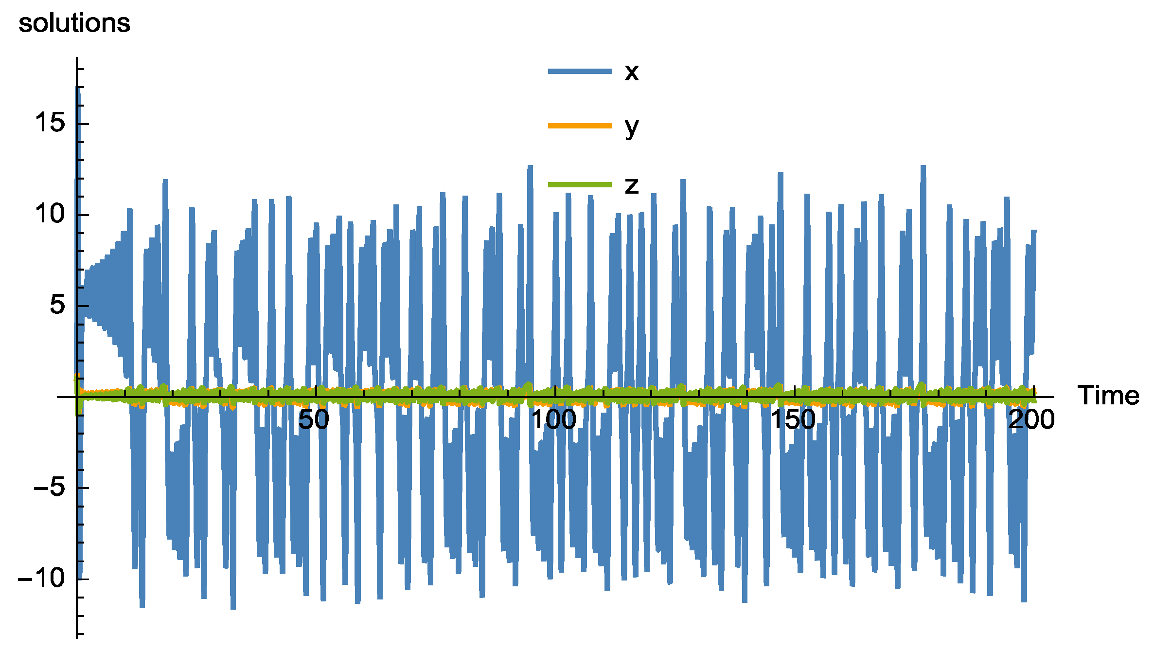
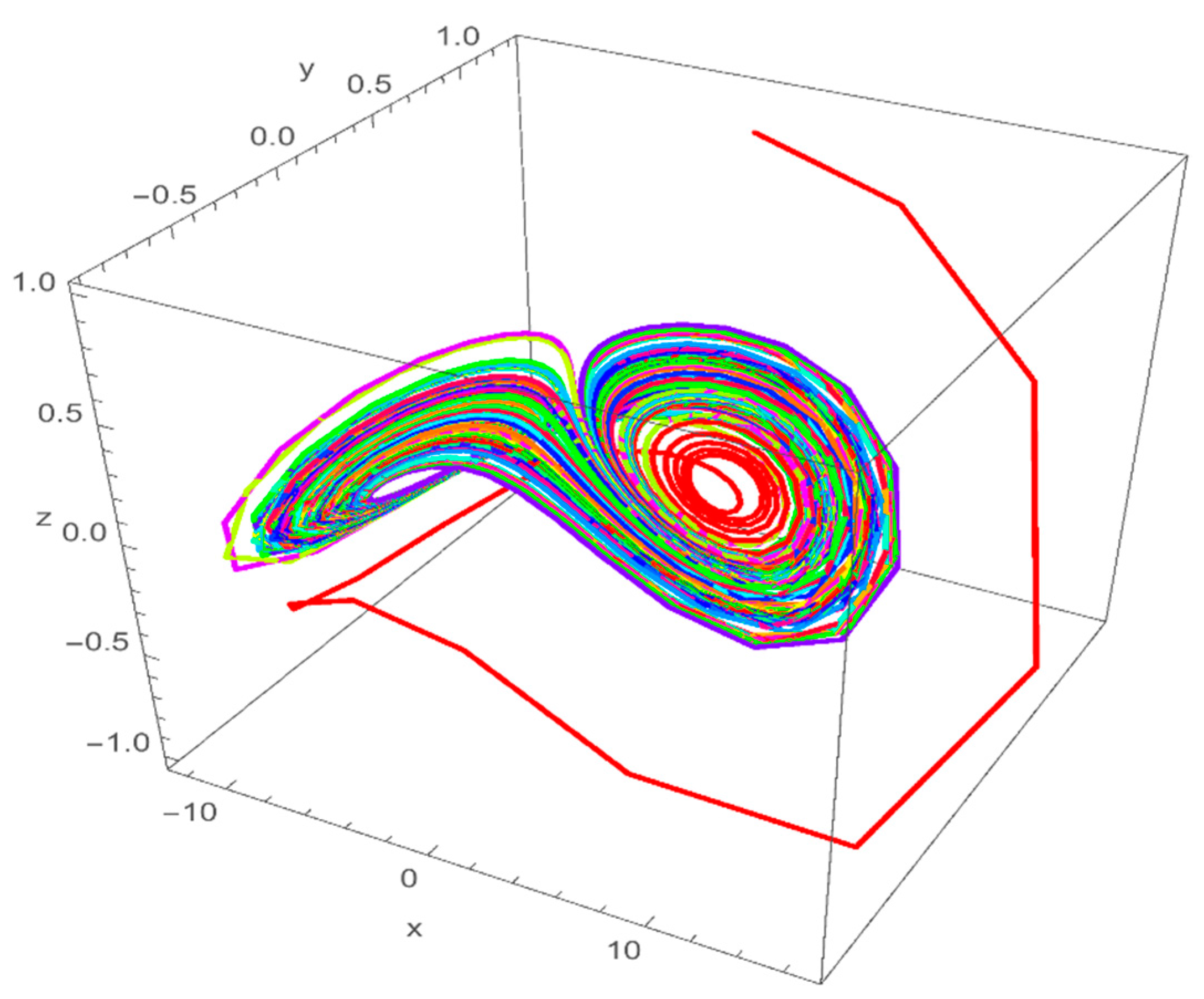
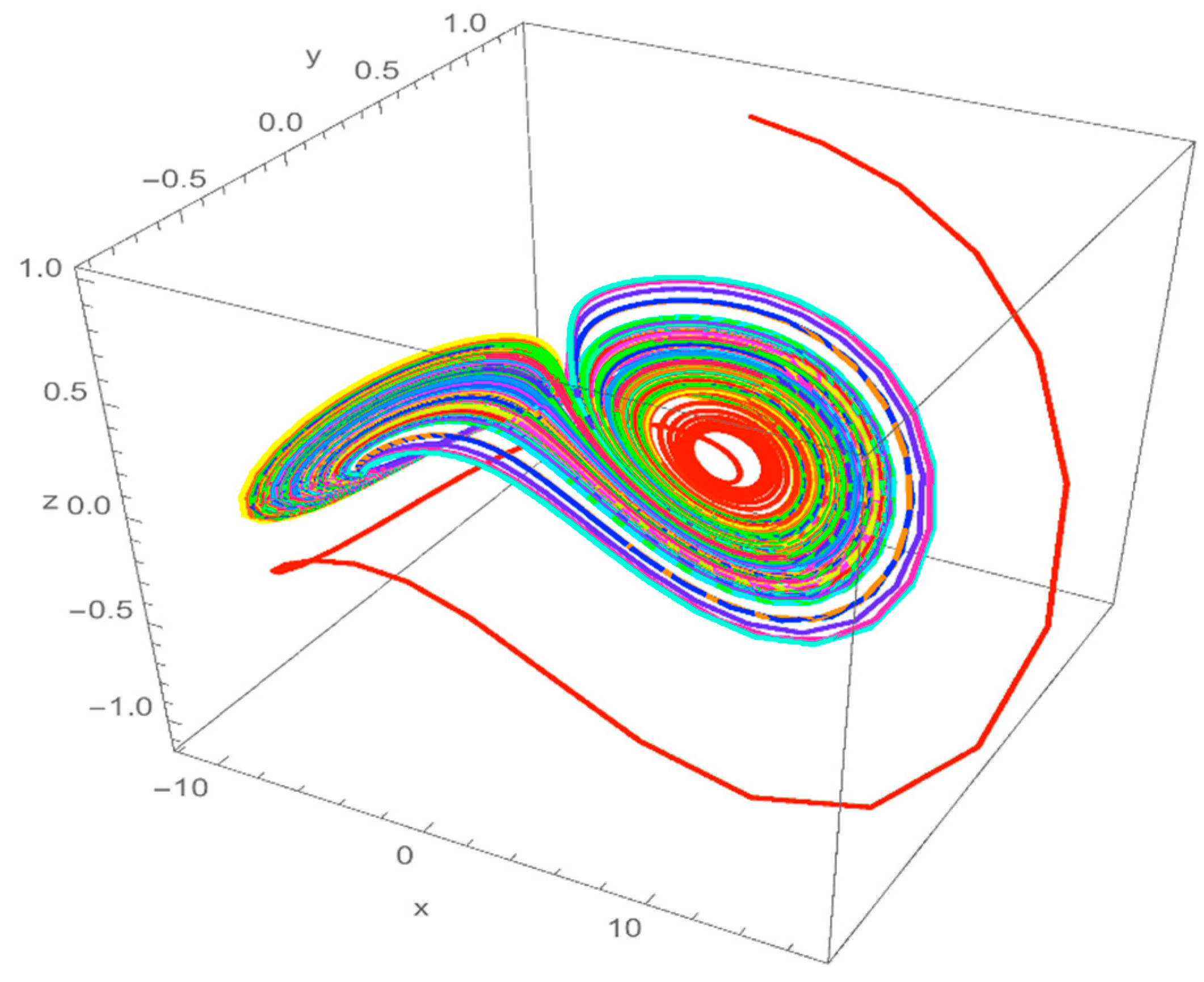
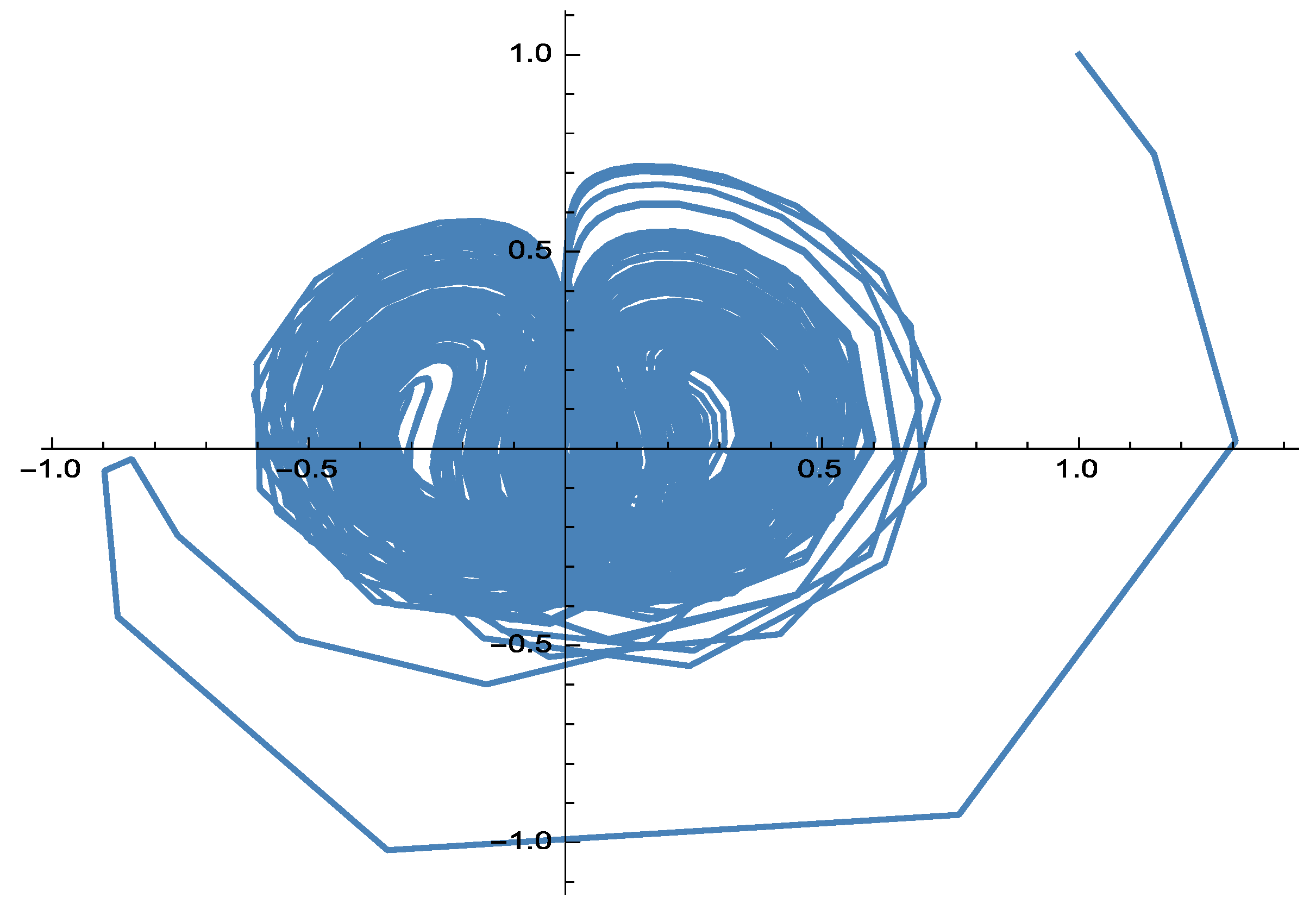
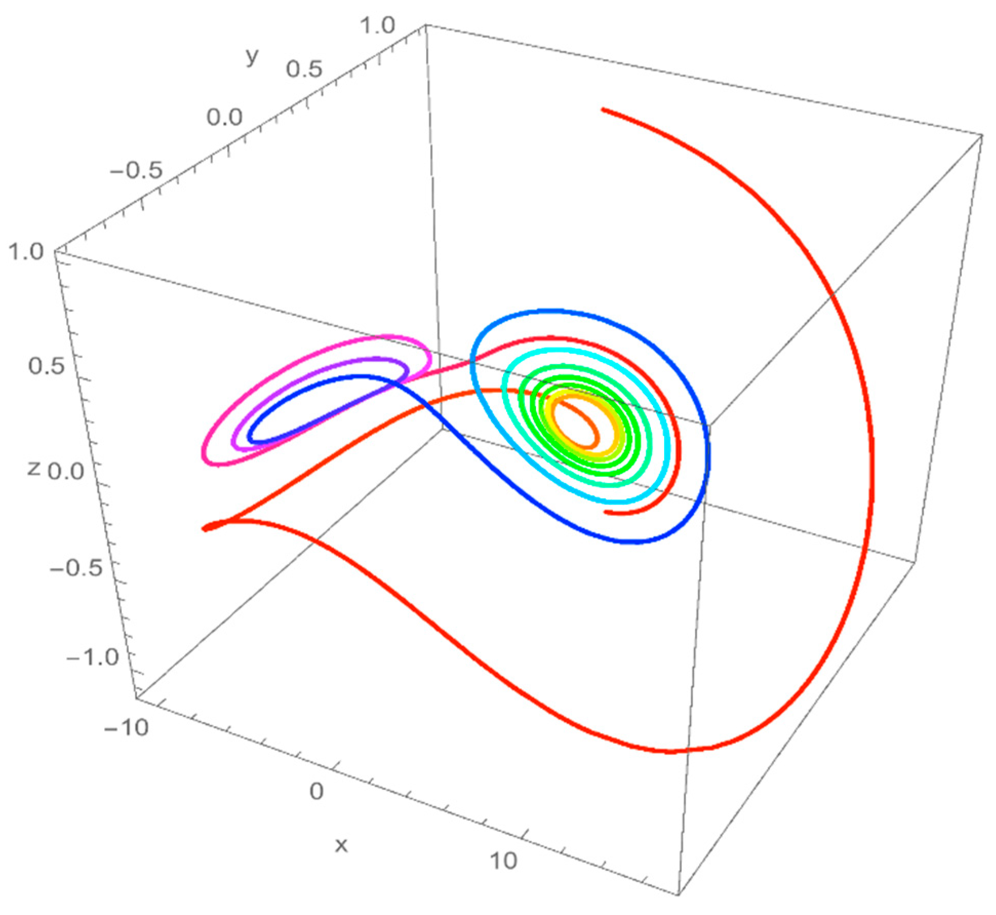
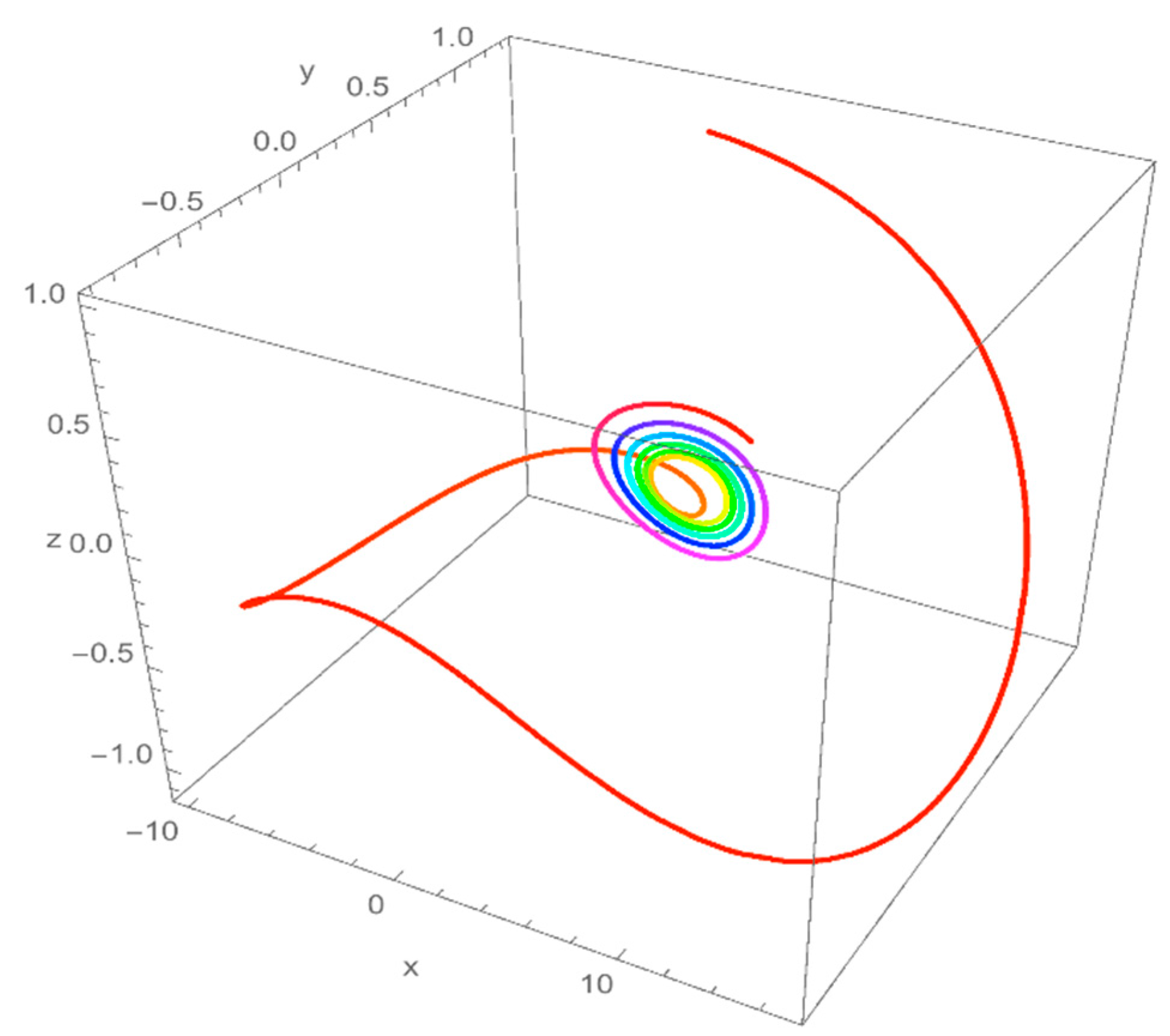
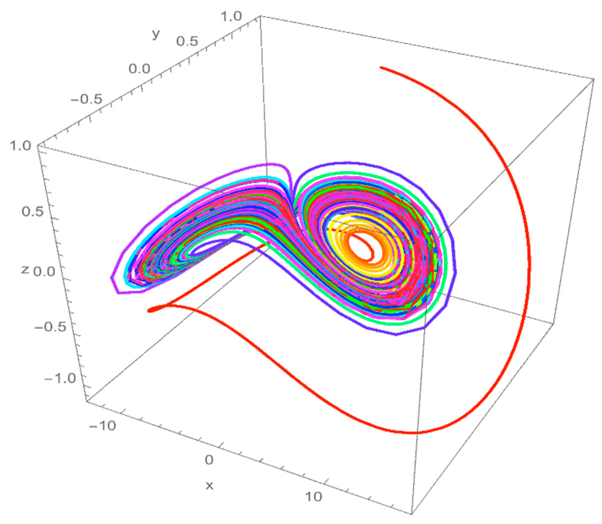
The numerical simulations are depicted in Figure 1, Figure 2, Figure 3, Figure 4, Figure 5 and Figure 6. In Figure 1 and Figure 2 we have the solution of the system 1. In Figure 3 and Figure 4, we have the 3 dimensional parametric plot of the system solution. In Figure 5 and Figure 6 we have the solution for y and z.
3. Analysis of Vallis Model with Caputo Derivative
In this section, we consider the model in system with the Caputo fractional derivative. Then system (1) becomes:
We derive the approximate solution of the above equation using the Laplace transform operator. Thus applying it on both sides of (23), we obtain:
By application of inverse Laplace on above system, we get:
The following iterative formula is then proposed:
The approximate solution is assumed to be obtain as a limit when n tends to infinity:
Stability Analysis of the Iteration Method
In this section, we demonstrate that the used method is stable when solving system (1). In this section, we assume the following: It is possible to find three positive constant A, W and J such that for all 0 ≤ t ≤ T ≤ ∞, and . We next consider a subset of defined by:
We now consider the following operator V defined as:
Then:
where and for all .
Thus applying the absolute value on both sides, the right hand side produces:
Then:
With:
Also if we consider a given non-null vector (X, Y, Z), then using the same routine as above we obtain:
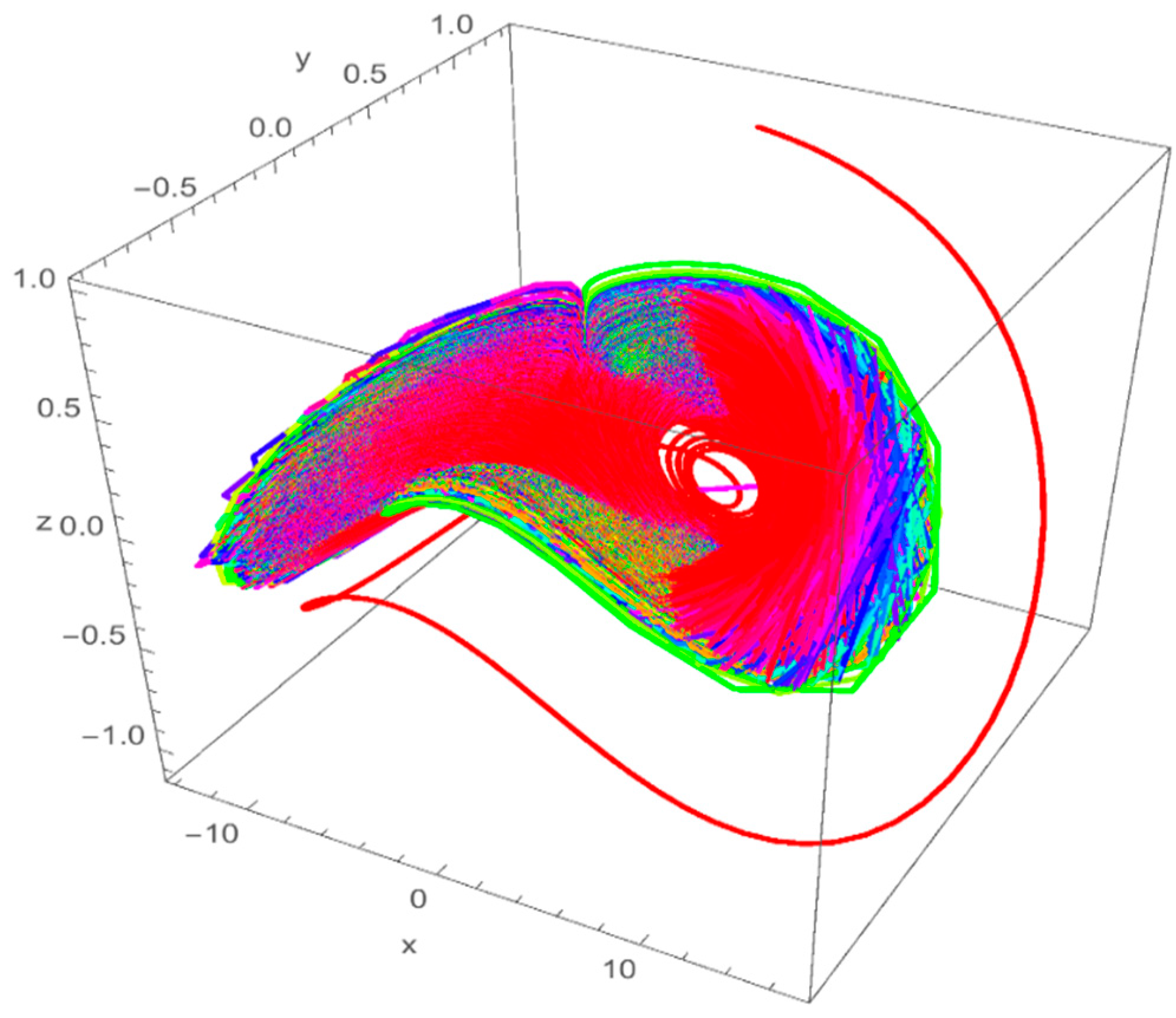
From the results obtained in Equations (30) and (31), we conclude that the used iterative method is stable. Using the iterative formula in (26) we present the numerical solution in Figure 7, Figure 8 and Figure 9 for different values of α. In these simulations, we used p = 0.3, with the nitial condition z(0) = y(0) = x(0) = 1.
From the above figures and with comparison with the model with local derivative, one can see that the Caputo derivative filters all high frequencies, as the order of α tends to zero. The Caputo derivative therefore plays a role of low band filter in this model.
4. Analysis of the Vallis Model with Caputo–Fabrizio Derivative
Some moderately current outcomes as of deterministic chaos field have extensive consequence for experts of information theory. Theory of information may be applicable to representational encodings of the phase-space descriptions of physical non-linear dynamical systems so that the characterization of process in terms of its Kolmogorov–Sinai entropy.
Consequently this concept of deterministic information theory happens to deal with way for assessing the limits of compression for single finite strings, while deterministic chaos theory results further permit one to choose particularly calibrated information sources to be employed to assess the performance of specific compression algorithm.
Since any novel applied mathematical concept must be entirely underpinned by some potential applications, we are here fully here with the concept of fractional derivative with no singular kernel Some result obtained via informations theory are used to define a new family of generalized informational entropies which are indexed by a parameter clearly related to fractals, via fractional calculus, and which is quite relevant in the presence of creation of uncertainty, via defects of the observation process. The relation with Shannon’s entropy, Renyi’s entropy and Tsallis’ entropy is clarified, and it is shown that Tsallis’ generalized logarithm has a direct significance in terms of fractional calculus.
In this section we consider the model in system with Caputo–Fabrizio derivative with fractional order. Thus the model in system one becomes:
where is the Caputo–Fabrizio derivative with fractional order defined in Equation (1). To derive a special solution for the above system, we employ the Sumudu transform operator. The relation between the Sumudu transform denoted by S and the Caputo–Fabrizio derivative with fractional order was developed in [20] as:
Therefore applying the Sumudu transform on both sides of system (32) yields:
Applying the inverse Sumudu transform on both sides, we obtain:
From the above, the following recursive method is proposed:
And as before the approximate solution can be obtained as:
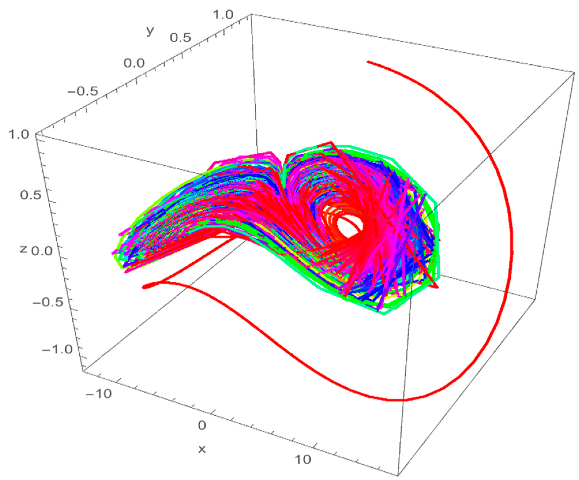
The stability analysis and existence of exact solutions for this model can be achieved similarly as before. However using the iteration formula suggested in (36) with initial conditions and p = 0.3, we present the numerical solution of system (32) for different values of α in Figure 10, Figure 11 and Figure 12. The initial conditions are the same as before.
Unlike the model with Caputo and local derivative, the model with Caputo–Fabrizio portrays more chaotic behavior as α is closer to 1, however when α is closer to zero we obtain approximately the chaotic behavior observed from the model with local derivative. Figure 10 and Figure 11 show a new chaotic behavior, which are not shown by the local derivative.
5. Conclusions
The Vallis model for El Niño was considered with three-different definitions of derivative in this work. We used the local derivative in one model, the Caputo derivative with power function kernel with singularity and the Caputo–Fabrizio derivative with exponential kernel, which has no singularity [21,22,23,24]. We presented the existence and uniqueness of the model with local derivative and then we derived approximate solutions via iterative method. We presented some numerical simulation and observed some chaotic behavior as p changes from zero to 0.3. We derived the solution of the model with Caputo derivative using the combination of Laplace transform and iterative formula. We presented the stability analysis of the used method together with some numerical simulations. The model with Caputo–Fabrizio was solved with Sumudu transform operator. We observed that the Caputo derivative played a role of high band filter, when the Caputo–Fabrizio shows more interesting chaotic behavior as α tends to 1.
Acknowledgments
The authors would like to extend their sincere appreciation to the Deanship of Scientific Research at King Saud University for funding this group No. RG-1437-017.
Author Contributions
Both authors contributed equally to this work. Both authors have read and approved the final manuscript.
Conflicts of Interest
The authors declare no conflict of interest.
References
- Tenreiro Machado, J.A. Entropy analysis of integer and fractional dynamical systems. Nonlinear Dyn. 2010, 62, 371–378. [Google Scholar] [CrossRef]
- Tenreiro Machado, J.A. Entropy analysis of fractional derivatives and their approximation. J. Appl. Nonlinear Dyn. 2012, 1, 109–112. [Google Scholar] [CrossRef]
- Ibrahim, R.W. The fractional differential polynomial neural network for approximation of functions. Entropy 2013, 15, 4188–4198. [Google Scholar] [CrossRef]
- Mathai, A.M.; Haubold, H.J. On a generalized entropy measure leading to the pathway model with a preliminary application to solar neutrino data. Entropy 2013, 15, 4011–4025. [Google Scholar] [CrossRef]
- Jalab, H.A.; Ibrahim, R.W. Denoising algorithm based on generalized fractional integral operator with two parameters. Discret. Dyn. Nat. Soc. 2012, 2012, 529849. [Google Scholar] [CrossRef]
- Jalab, H.A.; Ibrahim, R.W. Texture enhancement based on the Savitzky-Golay fractional differential operator. Math. Probl. Eng. 2013, 2013, 149289. [Google Scholar] [CrossRef]
- Vallis, G.K. El Niño: A chaotic dynamical system? Science 1986, 232, 243–255. [Google Scholar] [CrossRef] [PubMed]
- Letellier, C.; Dutertre, P.; Gouesbet, G. Characterization of the Lorenz system, taking into account the equivariance of the vector field. Phys. Rev. E 1994, 49. [Google Scholar] [CrossRef]
- Mischaikow, K.; Mrozek, M. Chaos in the Lorenz equations: A computer assisted proof. Part II: Details. Math. Comput. Am. Math. Soc. 1998, 67, 1023–1046. [Google Scholar] [CrossRef]
- Galias, Z.; Zgliczyński, P. Computer assisted proof of chaos in the Lorenz equations. Physica D 1998, 115, 165–188. [Google Scholar] [CrossRef]
- Magin, R.L.; Abdullah, O.; Baleanu, D.; Zhou, X.J. Anomalous diffusion expressed through fractional order differential operators in the Bloch–Torrey equation. J. Magn. Reson. 2008, 190, 255–270. [Google Scholar] [CrossRef] [PubMed]
- Cloot, A.; Botha, J.F. A generalised groundwater flow equation using the concept of non-integer order derivatives. Water SA 2006, 32, 1–7. [Google Scholar] [CrossRef]
- Caputo, M. Linear models of dissipation whose Q is almost frequency independent—II. Geophys. J. Int. 1967, 13, 529–539. [Google Scholar] [CrossRef]
- Benson, D.A.; Wheatcraft, S.W.; Meerschaert, M.M. Application of a fractional advection-dispersion equation. Water Resour. Res. 2000, 36, 1403–1412. [Google Scholar] [CrossRef]
- Berkowitz, B.; Cortis, A.; Dentz, M.; Scher, H. Modeling non-Fickian transport in geological formations as a continuous time random walk. Rev. Geophys. 2006, 44, 22–30. [Google Scholar] [CrossRef]
- Samko, S.G.; Kilbas, A.A.; Marichev, O.I. Fractional Integrals and Derivatives; Gordon and Breach Science Publishers: Yverdon, Switzerland, 1993. [Google Scholar]
- Caputo, M.; Fabrizio, M. A new definition of fractional derivative without singular kernel. Progr. Fract. Differ. Appl. 2015, 1, 73–85. [Google Scholar]
- Jorge, L.; Nieto, J.J. Properties of a new fractional derivative without singular kernel. Progr. Fract. Differ. Appl. 2015, 1, 87–92. [Google Scholar]
- Atangana, A. On the new fractional derivative and application to nonlinear Fisher’s reaction-diffusion equation. Appl. Math. Comput. 2016, 273, 948–956. [Google Scholar] [CrossRef]
- Atangana, A.; Nieto, J.J. Numerical solution for the model of RLC circuit via the fractional derivative without singular kernel. Adv. Mech. Eng. 2015, 7. [Google Scholar] [CrossRef]
- Gómez-Aguilar, J.F.; Yépez-Martínez, H.; Calderón-Ramón, C.; Cruz-Orduña, I.; Escobar-Jiménez, R.F.; Olivares-Peregrino, V.H. Modeling of a Mass-Spring-Damper System by Fractional Derivatives with and without a Singular Kernel. Entropy 2015, 17, 6289–6303. [Google Scholar] [CrossRef]
- Goufo, E.F.D.; Pene, M.K.; Mwambakana, J.N. Duplication in a model of rock fracture with fractional derivative without singular kernel. Open Math. 2015, 13. [Google Scholar] [CrossRef]
- Gómez-Aguilar, J.F.; López-Lópezb, M.G.; Alvarado-Martínezb, V.M.; Reyes-Reyesb, J.; Adam-Medinab, M. Modeling diffusive transport with a fractional derivative without singular kernel. Physica A 2016, 447, 467–481. [Google Scholar] [CrossRef]
- Alsaedi, A.; Baleanu, D.; Etemad, S.; Rezapour, S. On coupled systems of time-fractional differential problems by using a new fractional derivative. J. Funct. Spaces 2016, 2016, 4626940. [Google Scholar] [CrossRef]
Figure 1.
Solution as function of time for p = 0.3.

Figure 2.
Solution as function of time for p = 0.

Figure 3.
Parametric for p = 0.3.

Figure 4.
Parametric plot for p = 0.

Figure 5.
2-Dimensional parametric plot of y(t) and z(t) for p = 0.3.

Figure 6.
2-Dimensional parametric plot of y(t) and z(t) for p = 0.3.

Figure 7.
3-Dimensional representation for α = 0.85.

Figure 8.
3-Dimensional representation for α = 0.55.

Figure 9.
3-Dimensional representation for α = 0.25.
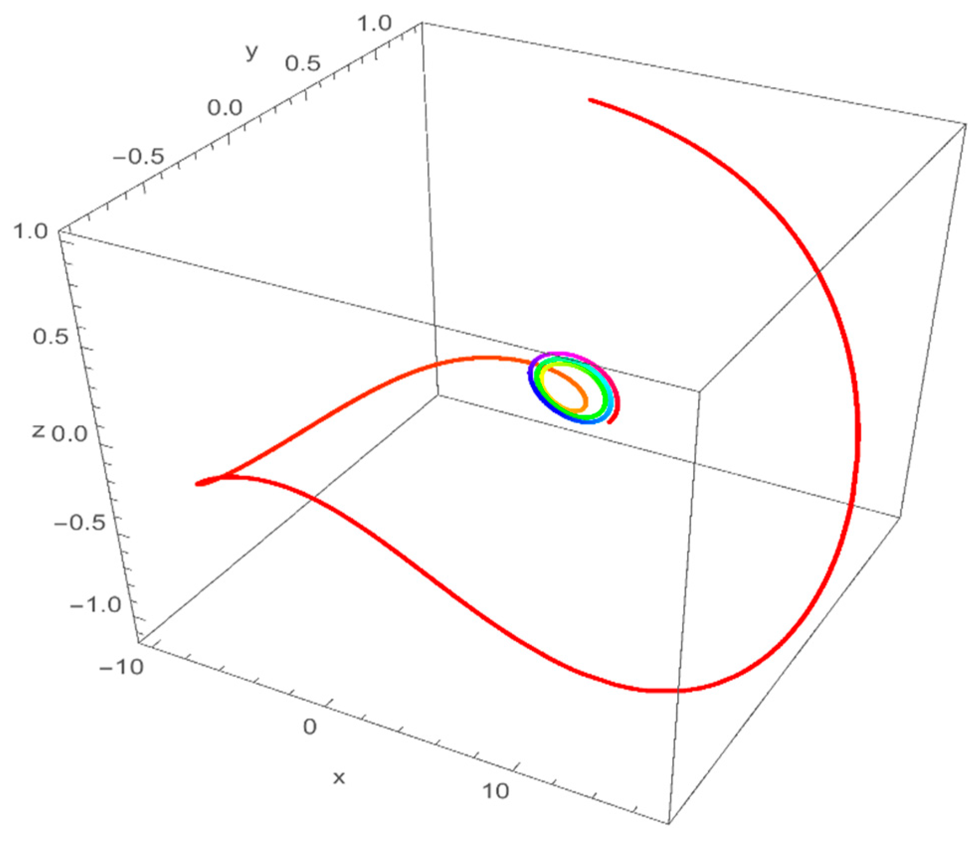
Figure 10.
3-Dimensional representation for α = 0.85.

Figure 11.
3-Dimensional representation for α = 0.55.

Figure 12.
3-Dimensional representation for α = 0.25.

© 2016 by the authors; licensee MDPI, Basel, Switzerland. This article is an open access article distributed under the terms and conditions of the Creative Commons by Attribution (CC-BY) license (http://creativecommons.org/licenses/by/4.0/).
Share and Cite
MDPI and ACS Style
Alkahtani, B.S.T.; Atangana, A. Chaos on the Vallis Model for El Niño with Fractional Operators. Entropy 2016, 18, 100. https://doi.org/10.3390/e18040100
AMA Style
Alkahtani BST, Atangana A. Chaos on the Vallis Model for El Niño with Fractional Operators. Entropy. 2016; 18(4):100. https://doi.org/10.3390/e18040100
Chicago/Turabian StyleAlkahtani, Badr Saad T., and Abdon Atangana. 2016. "Chaos on the Vallis Model for El Niño with Fractional Operators" Entropy 18, no. 4: 100. https://doi.org/10.3390/e18040100
Note that from the first issue of 2016, this journal uses article numbers instead of page numbers. See further details here.