A Hybrid EEMD-Based SampEn and SVD for Acoustic Signal Processing and Fault Diagnosis

Abstract

Acoustic signals are an ideal source of diagnosis data thanks to their intrinsic non-directional coverage, sensitivity to incipient defects, and insensitivity to structural resonance characteristics. However this makes prevailing signal de-nosing and feature extraction methods suffer from high computational cost, low signal to noise ratio (S/N), and difficulty to extract the compound acoustic emissions for various failure types. To address these challenges, we propose a hybrid signal processing technique to depict the embedded signal using generally effective features. The ensemble empirical mode decomposition (EEMD) is adopted as the fundamental pre-processor, which is integrated with the sample entropy (SampEn), singular value decomposition (SVD), and statistic feature processing (SFP) methods. The SampEn and SVD are identified as the condition indicators for periodical and irregular signals, respectively. Moreover, such a hybrid module is self-adaptive and robust to different signals, which ensures the generality of its performance. The hybrid signal processor is further integrated with a probabilistic classifier, pairwise-coupled relevance vector machine (PCRVM), to construct a new fault diagnosis system. Experimental verifications for industrial equipment show that the proposed diagnostic system is superior to prior methods in computational efficiency and the capability of simultaneously processing non-stationary and nonlinear condition monitoring signals.

1. Introduction

As a fundamental way of characterizing the condition of a mechanical system, diagnostics should fulfill the requirement of being able to detect all possible faults. As a defective component may run for certain time before it is totally damaged, the early detection of machinery fault and making corresponding maintenance arrangements have great impact on the reduction of unexpected shutdown and operation cost.

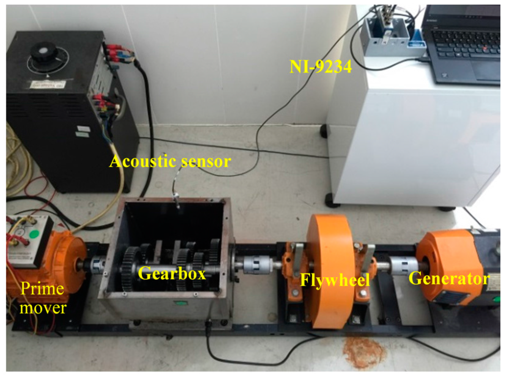
The condition monitoring process includes the acquisition of information, signal processing and pattern recognition. Various signal types, including vibrations, acoustic signals, and temperature, have been used for fault diagnosis. Considering the advantages of acoustic signals, there has been a tendency to apply acoustic signal analysis to machinery fault detection and diagnosis [1]. Firstly, acoustic signals are non-directional which means that one acoustic sensor can satisfy the data collection requirements, while signals on three axes are needed to be considered if using a vibration sensor. Secondly, acoustic signals are relatively independent of structural resonances [1]. 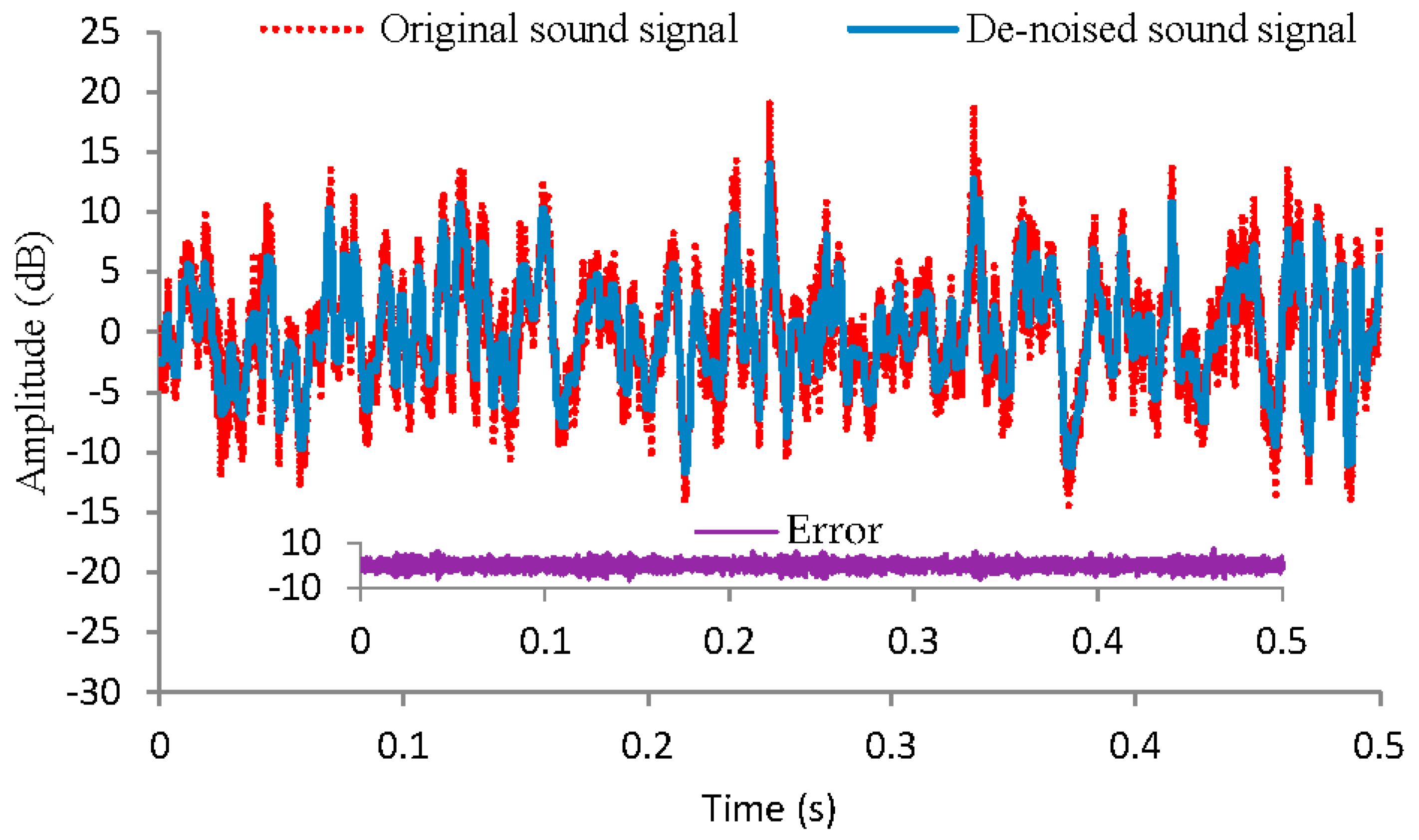Thirdly, the high sensitivity of acoustic signals [2] provides an opportunity to identify faults at an early stage [3]. What comes along with the benefits of acoustic signals are their problems of low signal to noise ratio (S/N) and high computational cost. As acoustic sensors can capture a much broader range of frequencies than vibration accelerometers, the S/N of acoustic signals is generally lower than that of vibrations. The high sampling frequency of acoustic signal which results from the high frequency of acoustic signals also make it undesirable to use long monitoring times because of the high computational cost, making the S/N even lower. It is thus imperative to adapt methods which reduce the computational time and increase the S/N when using longer monitoring times.

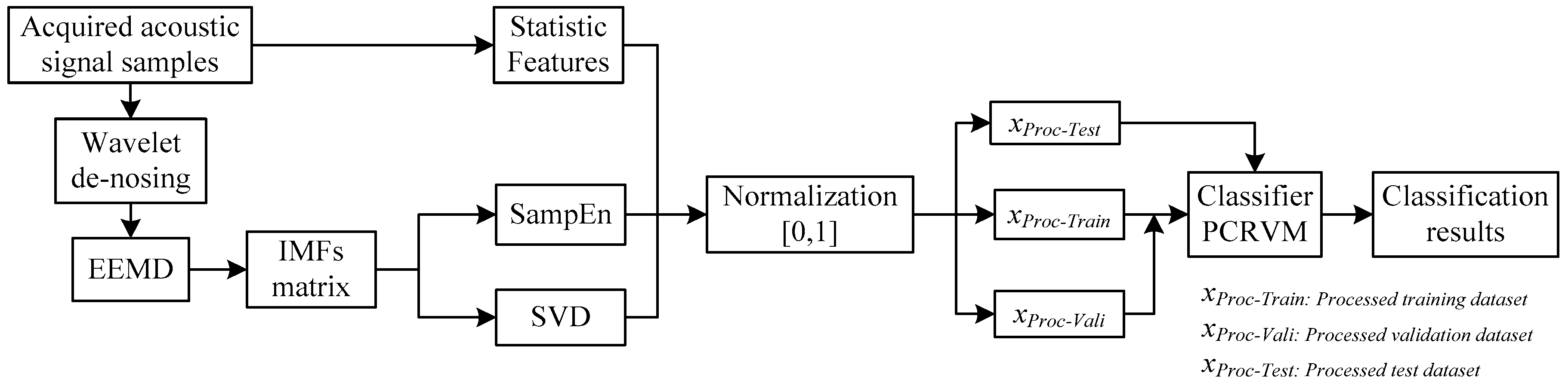
To overcome these problems, effective acoustic signal de-nosing techniques and suitable feature extraction methods are adopted. In this study, a widely used method, discrete wavelet transform (DWT) using soft threshold [4], is adopted. In addition, some time-frequency analysis methods, including wavelet transorm and empirical mode decomposition (EMD), are adopted for fault feature extraction from rotating machinery signals [5]. The wavelet transform is the most dominant method used nowadays [6], but it still has many defects to overcome. First, as a wavelet transform is in fact a windowed Fourier transform, energy leakage will occur during the signal processing. Second, once the decomposition scales are determined, the wavelet transform result is the signal under a certain frequency band. In other words, a wavelet transform is not a self-adaptive signal processing method by nature [7]. 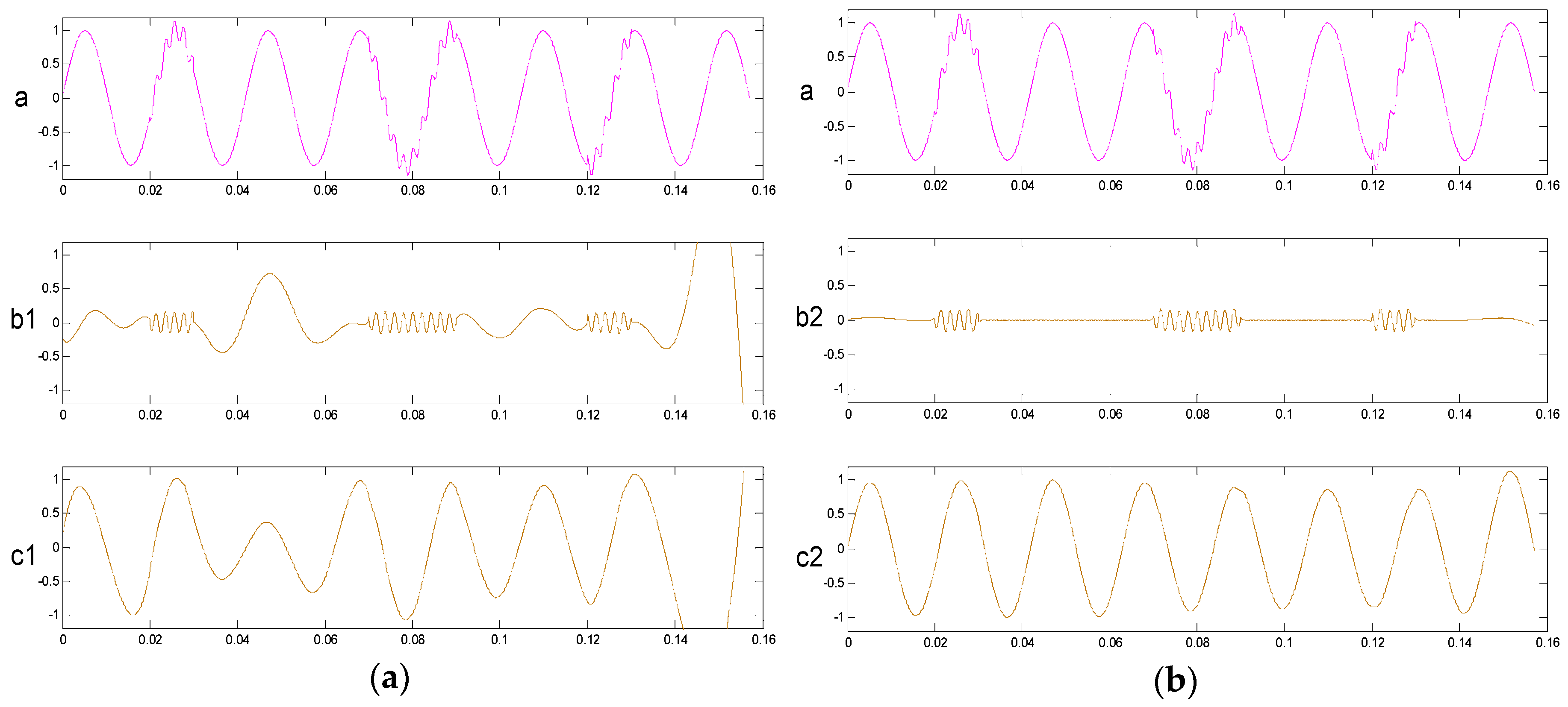EMD has been proposed as a time-frequency signal processing technique to deal with non-linear and non-stationary problems as in this application [8]. It decomposes a complicated signal into a series of intrinsic mode functions (IMFs) which not only relate to the sampling frequency, but change with the signal itself. Hence, it is a kind of adaptive signal processing technique for non-linear and non-stationary signals. However, the major disadvantage of EMD is the issue of mode mixing. 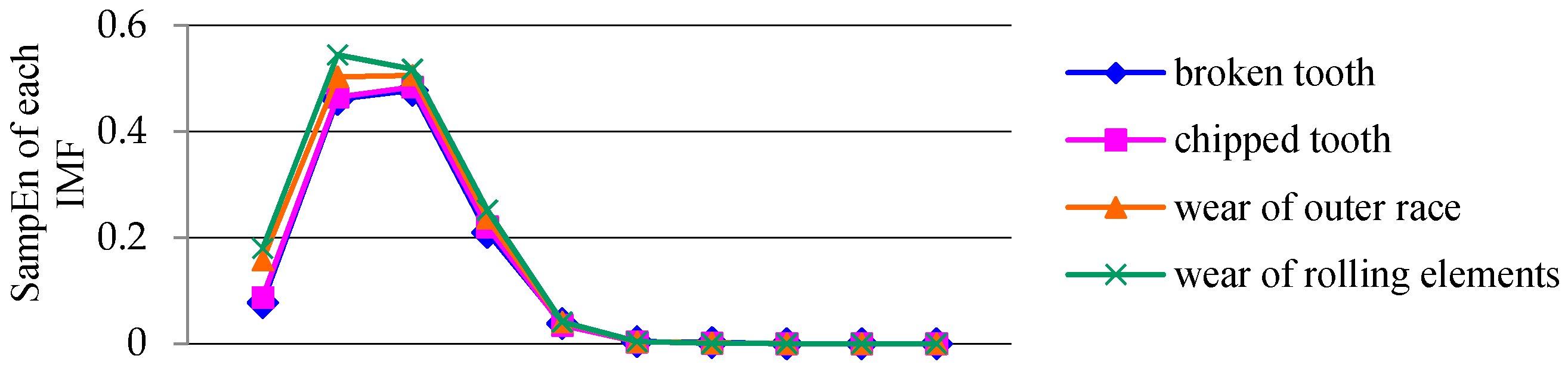To overcome the issue, an improved EMD method, ensemble empirical mode decomposition (EEMD), was recently proposed by Wu and Huang [9]. EEMD is a noise-assisted data analysis method that involves adding finite white noise to the investigated signal to eliminate the mode mixing problem. Compared with the aforementioned signal processing methods, EEMD is proposed as a suitable time-frequency analysis technique to process acoustic signals in this application. Even though EEMD decomposes the signals into IMFs containing the local features of a signal, however, the data size of IMF is the same as that of the raw data, which is usually very big. Therefore, a proper feature selection method should be also considered in the feature extraction phase to determine representative features from IMFs so as to reduce the input dimensions of the classifier.

In the previous literature, both the sample entropy (SampEn) [10,11] and singular value decomposition (SVD) [12] methods are adopted to extract the representative characteristics from IMFs. Generally, different indicators can be used to describe different failures. For example, a broken tooth in a gear has a relatively regular acoustic signal because it is periodic, so the outcome of SampEn is relatively low, which is very similar to the outcome of a periodic fault such as chipped tooth because as an indicator SampEn mainly describes the regularity not the detailed impulse. This makes it easier to produce a wrong classification. On the contrary, SVD can easily solve the problem by rendering the singular value matrix of the fault signal which can represent the periodic fault information adequately. As for a non-periodic signal such as outer race wear in a bearing, the signal is very unpredictable as its regularity is very low. In this case, the performance of SVD is worse than SampEn which can depict the fault properly by rendering the extent of its irregularity. A hybrid of the two approaches meets the needs of fault classification with high accuracy. In this paper, the authors propose a meritorious hybrid of SampEn and SVD, which are based on EEMD and assisted by the statistical features of the acoustic signals, that dramatically reduces the dimension of IMFs, allowing taking all meaningful IMFs into account and the use of long monitoring times, without increasing the computational expense, and at the same time, enhancing the classification accuracy to a considerable extent. After extracting the features based on SampEn and SVD, the extracted feature vectors are adopted to execute a pattern recognition algorithm.

Neural network-based monitoring systems have been proposed [13,14,15]. However, neural network (NN) classifiers have many limitations, including local minima problems, being time-consuming, and the risk of over-fitting. To date, researchers have already applied support vector machines (SVM) to engineering diagnosis problems [16,17], and have shown that SVM is superior to traditional NNs [18]. The major advantages of SVM are its global optimum and a higher generalization capability. Considering that there are more than two fault types always exist in a machinery system, it is necessary to find a suitable probabilistic classifier which can output the probability rank of all failures. According to the rank, the other possible faults can be traced when the prediction result is not right [19]. The probabilistic neural network (PNN) was proposed as a probabilistic classifier for multi-label classification [20]. However, with PNN it is difficult to deal with the issue of large-scale data such as the multiple acoustic signal problem presented in this paper. Recently, a probabilistic classifier, relevance vector machine (RVM), was proposed by Widodo et al. 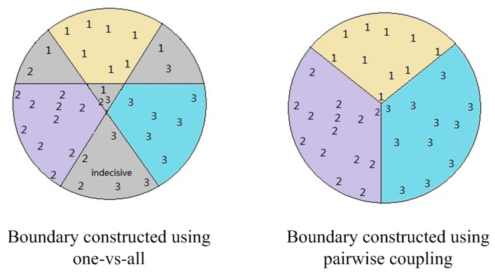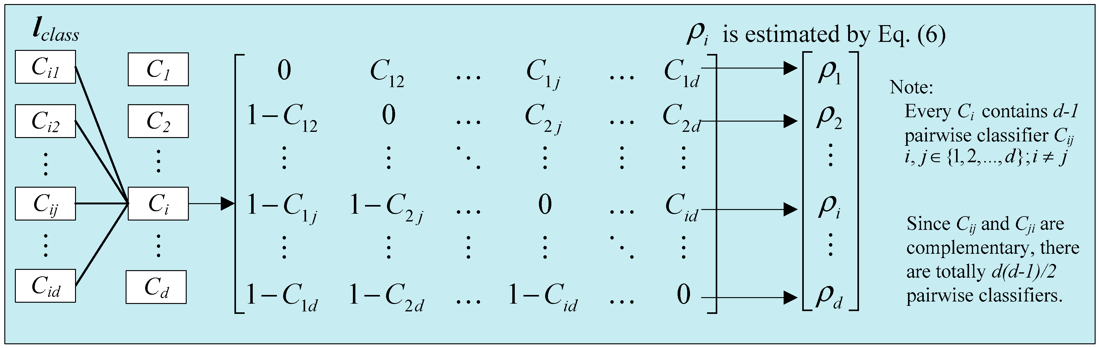[21] and Tipping [22] to deal with fault diagnosis of low speed bearings. To deal with the issue of multi-class classification, RVM is adopted in this application. A one-vs-all strategy is usually adopted to overcome the multi-class classification problem. However, this strategy was verified to produce a large indecision region [23,24]. The pairwise coupling strategy, one-vs-one, is introduced into RVM to overcome the drawback, leading to the concept of a pairwise-coupled relevance vector machine (PCRVM). Since the correlation between each pair of faults is considered by the pairwise coupling strategy, a more accurate estimation of the probability of the fault signal can be achieved. A detailed explanation of the advantages of the pairwise coupling strategy is presented in Section 2.3.

To summarize, a framework combining feature extraction (EEMD based SampEn and SVD), which is assisted by statistical features, and PCRVM is proposed for fault diagnosis. The original features of the work presented in this paper are summarized below:

• It is the new research that analyzes the properties of feature extraction using EEMD+SampEn, which is extremely effective for dealing with irregular faults while it can always improve the overall performance of fault diagnosis for all types of signals.
• It is the first example in the literature that observes the suitable application domain of EEMD+SVD method, which is sensitive for periodic faults and will not downgrade the classification accuracy for irregular faults.
• The proposed EEMD-based hybrid signal processing method, combined with SF, SampEn and SVD, provides a new and robust solution to improve the general performance of feature extraction and fault diagnosis systems for various kinds of signals.
• The proposed fault diagnosis framework, using the hybrid feature extraction module and the probabilistic classifier, pairwise-coupled relevance vector machine, can achieve a high diagnostic efficiency for simultaneous faults.

2. Methodology

The methodology is illustrated in four parts. The first part briefly introduces the signal pre-processing methods, including signal de-nosing (DWT) and signal decomposition (EEMD). SampEn is introduced and followed by SVD as approaches to reduce computational cost and enhance S/N in the second part. The third part demonstrates the meaning of the hybrid of SampEn and SVD and proposes an innovative framework. The last part is concerned with pattern recognition which introduces a probabilistic classifier PCRVM. Figure 1 shows a brief outline of the framework.

2.1. Data Processing

2.1.1. Signal Denosing

A discrete wavelet transform (DWT) using a soft threshold is selected in this paper. The soft threshold is calculated as sign (x) ($\left|x\right|-t$), if $\left|x\right|>t$, and otherwise is 0, where t denotes the threshold [25]. More details on the denoising procedures are described in Section 3.2.

2.1.2. Empirical Mode Decomposition (EMD)

EMD is defined that any complicated signal that can be transformed into several IMF components. After implementing the EMD, the original signal x(t) can be expressed as follows:

$$x(t)={\displaystyle \sum _{i=1}^n{c}_i(t)+r_n}(t)$$

(1)

where c_i(t) and r_n(t) are the ith IMF and residue, respectively. The ith IMF changes with the frequency of the signal from high to low; the residual term r_n(t) is usually overlooked because it represents the very low energy part of the signal. Although EMD has been widely adopted in signal processing for diagnostics, mode mixing degrades the performance of EMD in practical applications.

2.1.3. Ensemble Empirical Mode Decomposition (EEMD)

To overcome the problem of mode mixing, the EEMD is proposed by introducing the concept of noise-assisted data analysis. Generally speaking, when the investigated signal is dominated by high-frequency components, the noise amplitude needs to be smaller, and when the investigated signal is dominated by low-frequency components, the noise amplitude should be increased. The differences between the EEMD and EMD procedures are as follows:

(1)

Add different white noise to the original signal to get a group of synthesized signals.

(2)

Applying EMD to all the synthesized signals and get different groups of IMFs.

(3)

Calculate the mean of corresponding IMF to generate the final result.

A simulated experiment was conducted to illustrate the improvement provided by using EEMD. The simulation signal is a combination of a sine wave and small impulses. By applying EMD and EEMD to the simulation signal, respectively, we obtained IMF(b1) and IMF(c1) in Figure 2a and IMF(b2) and IMF(c2) in Figure 2b. It can be seen in Figure 2a that both IMF(b1) and IMF(b2) could not represent the sine wave nor the impulses perfectly. Mode mixing happens between the two components, resulting in the fact that the two components reside in each other. From IMF(b2) and IMF(c2) in Figure 2b, it is shown that EEMD overcomes the mode mixing issue.

2.2. Dimension Reduction and S/N Enhancement

Computational efficiency has been the focus of almost all algorithms, which still holds in our case. There are three main reasons why dimension reduction is imperative in our work. The first is that we adopt acoustic signals as the input signal which have much higher frequency than vibrations, enlarging the sample dataset and limiting the monitoring time of each sample. The second reason is that many trials are required due to the additional noise process of EEMD. The last one is that EEMD decomposes the original signal into many IMFs which makes the dataset at least ten times larger than before. At the meantime, the S/N of acoustic signals is generally lower than that of vibrations, making it inconvenient to classify different types of faults.

2.2.1. Sample Entropy

Sample entropy (SampEn) is a modification of approximate entropy [26]. It is used to evaluate the degree of information production. SampEn can be calculated as follows:

$$\text{SampEn}(m,r,N)=\text{ln}[\frac{1}{N-m+1}{\displaystyle \sum _{i=1}^{N-m+1}{C}_r^m(i)}-\frac{1}{N-(m+1)+1}{\displaystyle \sum _{i=1}^{N-(m+1)+1}{C}_r^{m+1}(i)}]$$

(2)

where N is the length of signals, m is the match of length, and $C_r^m(i)$ is the probability that any two epochs match each other. By choosing a proper noise filter parameter r (usually chosen around 25% of the standard deviation of the signal) it is possible to eliminate the effect of noise [27].

In the proposed framework, SampEn selects the features from IMFs to combine as extracted features, x_SE = [SampEn₁, SampEn₂,…, SampEn_n] where n is the number of IMFs. The extracted features will be sent to the classifier as indicator vectors.

2.2.2. Singular Value Decomposition (SVD)

SVD is a linear algebra technique that is employed to analyze matrices. In SVD, any matrix X of size I × N can be decomposed into three matrices, which are defined as follows:

$$X=U\mathsf{\Lambda }{V}^T$$

(3)

where U and V are orthogonal matrices, $\mathsf{\Lambda }$ is a diagonal matrix in which the diagonal element ${\mathsf{\sigma }}_i$ represents the singular values of X. The singular values are listed in the descending order automatically, ${\mathsf{\sigma }}_1\left(X\right)\ge {\mathsf{\sigma }}_2\left(X\right)\ge \cdots \ge {\mathsf{\sigma }}_I\left(X\right)$, by SVD function:

$$\mathsf{\Lambda }=\left[\begin{array}{cccc}{\sigma }_1& 0& \cdots & 0\\ 0& {\sigma }_2& & 0\\ ⋮& & \ddots & ⋮\\ 0& 0& \cdots & {\sigma }_I\end{array}\right]$$

(4)

After the application of SVD to IMF matrix X, the singular values $\mathsf{\sigma }\left(X\right)$ of X, which contains the fault feature vector, can be obtained as follows:

$$\sigma (X)=[{\sigma }_1(X),{\sigma }_2(X),\cdots ,{\sigma }_I(X)]$$

(5)

The fault is then identified and classified according to the obtained fault feature vector $\mathsf{\sigma }\left(X\right)$. When the features describing the characteristics of the signals are available, the next step is to construct the probabilistic committee machine based on the obtained features.

2.3. Pairwise-Coupling Relevance Vector Machine

Relevance vector machine (RVM) has shown its advantages over traditional classifiers and thus has attracted more and more attention in diagnostics [28]. By utilizing a Bayesian learning framework and popular kernels, RVM has the ability to produce probabilistic outcomes. In modern industry, there are always more than two types of fault that could occur in one system, but the traditional RVM formulation uses the one-vs-all strategy to overcome the problem of binary classification, which is not qualified for fault diagnosis. Taking the d-label issue as example, the one-vs-all strategy builds d classifiers l_class = [C₁, C₂,…C_i,…, C_d]. For any undefined input x, the classification vector G = [G₁, G₂,…G_i,…, G_d], where G_i= 1 if C_i(x) = +1 or G_i= 0 if C_i(x) = −1. Although the one-vs-all strategy is simple to implement, it generally provides a poor performance [28,29] because the pairwise correlation of each label is not considered, which creates a larger indecision region as shown in Figure 3. On the other hand, pairwise coupling (one-vs-one) also builds d classifiers l_class = [C₁,C₂,…C_i,…, C_d] for a d-label issue in which each C_i = [C_i1, C_i2,…C_ij,…, C_id] contains d − 1 different pairwise classifiers C_ij, i ≠ j. In other words, a total of d(d − 1)/2 classifiers is constructed in l_class as shown in Figure 4. The output vector of probability ${\rho }_i$ is defined as:

$${\rho }_i=C_i(\mathit{x})=\frac{{\displaystyle \sum _{i=1:i\ne j}^d{n}_{ij}{C}_{ij}(\mathit{x})}}{{\displaystyle \sum _{j=1:i\ne j}^d{n}_{ij}}}=\frac{{\displaystyle \sum _{j=1:i\ne j}^d{n}_{ij}{\rho }_{ij}}}{{\displaystyle \sum _{j=1:i\ne j}^d{n}_{ij}}}$$

(6)

where n_ij is the number of training feature vectors with either ith or jth labels. Considering the pairwise correlation between the faults, the proposed framework PCRVM can evaluate the vector of probability ${\rho }_i$ at a high accuracy level, and hence generates a higher classification accuracy.

3. Experimental Setup and Data Preparation for a Case Study

3.1. Test Rig and Sample Data Acquisition

The test rig includes a computer for data acquisition, an electric load simulator as prime mover, a gearbox, a flywheel, and an asynchronous generator, which is shown in Figure 5. It can simulate two periodic faults in the gearbox, a broken tooth and a chipped tooth, and two irregular faults, wear of outer race and rolling elements.

Table 1. The detailed descriptions of the four simulated cases.

Case No.	Description of Fault
C1	Broken tooth
C2	Chipped tooth
C3	Wear of outer race of bearing
C4	Wear of the rolling elements

shows the detailed descriptions of the four simulated faults. The acoustic sensor was located above the gearbox to record the four simulated faults with a sample rate of 25.6 kHz. The sampling rate was set to a relatively high frequency, which can ensure no signal is missed. In other words, every sampling data for each case has 25,600 data points. Finally, a total of 2000 fault samples (i.e., four simulated faults × 500 samples) was acquired. To test the diagnostic performance, the acquired signals were separated into three datasets as presented in

Table 2. Division of the sample dataset into different subsets. (Note that the feature extraction includes EEMD-based SampEn, EEMD-based SVD and statistic features.)

Raw Sample Data		Feature Extraction
Validation dataset	DValid (800)	Validation dataset	DProc_Valid (800)
Training dataset	DTrain (800)	Training dataset	DProc_Train (800)
Test dataset	DTest (400)	Test dataset	DProc_Test (400)

, where D_Valid denotes the validation set without feature extraction, D_{Proc_Valid} indicates the validation set of the extracted features.

3.2. Signal Denoising

The acoustic signal usually suffers from background noise interference. To improve the diagnostic performance, the acoustic signals need to be denoised. Through a series of experimental trials, the Daubechies mother wavelet with 4 levels “db4” and a soft threshold are adopted in this study. Considering the acoustic signal of a broken tooth as an example, the denoised result is demonstrated in Figure 6. The error means the difference between the original acoustic signal and denoised acoustic signal in which the white noise component of the signal can be readily eliminated. The result implies the wavelet shrinkage denoising method is effective and sufficient for signal denoising.

3.3. Feature Extraction

After denoising the signals, EEMD decomposes the acquired signal into I IMFs and residual signal r_I. The SampEn and SVD are adopt for extracting the features from the obtained IMFs. Furthermore, statistic feature indicators are extracted from the original signal as they are important in analyzing the acoustic signals. There are many statistical features available in the literature. Most of the features deal with the data distribution, such as peakiness, amplitude level, deviation from the mean and so on. These features provide the physical characteristics of time series data. In this study, 10 statistical features are employed to analyze the sound signal [30].

Table 3. Definition of the selected statistical features for acoustic signal.

Features	Equation	Features	Equation
1. Mean	$x_m=\frac{1}{N}{\displaystyle \sum _{i=1}^N{x}_i}$	6. Kurtosis	$x_{kur}=\frac{{\displaystyle \sum _{i=1}^N{(x_i-x_m)}^4}}{(N-1)x_{std}^4}$
2. Standard deviation	$x_{std}=\sqrt{\frac{{\displaystyle \sum _{i=1}^N{(x_i-x_m)}^2}}{N-1}}$	7. Crest factor	$CF=\frac{x_{pk}}{x_{rms}}$
3. Root mean square	$x_{rms}=\sqrt{\frac{1}{N}{\displaystyle \sum _{i=1}^N{x}_i^2}}$	8. Clearance factor	$CLF=\frac{x_{pk}}{{(\frac{1}{N}{\displaystyle \sum _{i=1}^N\sqrt{\left|x_i\right|}})}^2}$
4. Peak	$x_{pk}=\text{max}\left|x_i\right|$	9. Shape factor	$SF=\frac{x_{rms}}{\frac{1}{N}{\displaystyle \sum _{i=1}^N\left|x_i\right|}}$
5. Skewness	$x_{ske}=\frac{{\displaystyle \sum _{i=1}^N{(x_i-x_m)}^3}}{(N-1)x_{std}^3}$	10. Impulse factor	$IF=\frac{x_{pk}}{\frac{1}{N}{\displaystyle \sum _{i=1}^N\left|x_i\right|}}$

Note: x_i represents a signal series for i = 1,2,…, N, where N is the number of data points of a raw signal.

presents these statistical features.

As IMFs are listed in the descending order, the last few IMFs, which have a frequency lower than 0.5 Hz, have nothing to do with the fault information, and the SampEn of these IMFs are zero, which contributes almost nothing to the classification accuracy. As a result, the first 10 IMFs are adopted in this experiment.

3.4. Normalization

To ensure that all the features have even contribution, all reduced features should go through normalization. The interval of normalization is within [0,1] as follows:

$$y=\frac{(x-x_{\text{min}})}{(x_{\text{max}}-x_{\text{min}})}$$

(7)

where $x$ and y are the output feature and result of normalization, respectively. After normalization, a processed dataset x_Proc is obtained. The classifier can be trained by using x_Proc-TRAIN and the PCRVM method.

4. Results and Discussion

To compare the performance of different methods, a set of experiment results were obtained to determine the best combination of the proposed approaches.

4.1. Performance of Conventional Statistic Feature Indicators Using Denoised Signals

There are many condition indicators available in literature. The 10-SF are picked out as they depict the most traditional aspects of acoustic signals. In many vibration-concerned papers, the 10-SF are used alone as condition indicators, and their performance complies with the expectations perfectly, but in this paper, the signal we use is an acoustic signal which has quite a lot differences compared with vibrations, so the 10-SF are used alone as input condition indicators to be sent to PCRVM as a comparison. Moreover, to verify the effectiveness of the proposed denoising technique, denoised acoustic signals based on PCRVM are used to compare with the original signals. The experimental result is shown in

Table 4. Comparison of original and denoised signals using 10-SF.

Denoised Signals	Periodic Faults				Irregular Faults				Overall Result
	Broken Tooth		Chipped Tooth		Wear of Outer Race		Wear of Rolling Elements
	Original Signals	Denoised Signals	Original Signals	Denoised Signals	Original Signals	Denoised Signals	Original Signals	Denoised Signals	Original Signals	Denoised Signals
Correct cases	72	75	86	87	81	83	77	77	316	322
Wrong cases	28	25	14	13	19	17	23	23	84	78
Accuracy	72%	75%	86%	87%	81%	83%	77%	77%	79%	80.5%

.

As can be seen from Table 4, although the denoised signals using 10-SF give a 1.5% improvement compared with the original signals in the overall results, the accuracy of the result is a barely acceptable 80.5%. The reason why 10-SF performs much better when used in vibration analysis than when used here is that the noise ratio of vibration signals is generally lower than that of acoustic signals. The energy of the fault features in acoustic signals is much lower compared with vibrations, and as a result, 10-SF cannot extract the fault features properly to give a desirable outcome.

4.2. Results and Discussion of the Hybrid of SF and EEMD Based SampEn

To overcome the drawbacks of using the SF alone, the denoised acoustic signal should be inspected from other perspectives rather than only in a time-domain way. EEMD meets these needs very well. Compared with EMD, EEMD has no mode mixing problems. EEMD decomposes the acoustic signals into n IMFs which are listed in descending order of frequencies. IMFs represent the different components of the acoustic signals including the fault information. As the sample entropy can be extracted out by applying SampEn to each IMF, it can be compared to emboss the fault information to acquire a more accurate answer. To illustrate the advantages of EEMD, a comparison of EEMD- and EMD-based 10-SF and SampEn using denoised acoustic signals is shown in

Table 5. Comparison of the hybrid of 10-SF and EMD/EEMD-based SampEn.

Denoised Signals	Periodic Faults				Irregular Faults				Overall Result
	Broken Tooth		Chipped Tooth		Wear of Outer Race		Wear of Rolling Elements
	EMD	EEMD	EMD	EEMD	EMD	EEMD	EMD	EEMD	EMD	EEMD
Correct cases	80	83	90	90	94	95	93	93	357	361
Wrong cases	20	17	10	10	6	5	7	7	43	39
Accuracy	80%	83%	90%	90%	94%	95%	93%	93%	89.25%	90.25%

. As expected, by removing the mode mixing effects, the accuracy of EEMD is improved by 1% in the overall result as compared with the EMD. Therefore, the EEMD-based method is used in the following calculations.

Besides, compared with 10-SF using denoised signals in Table 4, EEMD with the SampEn method in Table 5 shows that the irregular faults, wear of outer race and the rolling elements, contribute the most to the improvement by eliminating 28 wrong cases, while the periodic faults, broken tooth and chipped tooth, contribute to the improvement of eight cases and three cases, respectively. In other words, the performance of EEMD with SampEn method in the irregular faults is superior than with the periodic faults. The reason for this is that the values of SampEn of the irregular faults, wear of outer race and rolling elements, are more different than those of the periodic faults, broken tooth and chipped tooth, which is shown in Figure 7. Thus, there is a great improvement of the classification accuracy of irregular faults. Taking the chipped tooth based on EEMD in Table 5 as an example, the 10 wrongly classified chipped tooth using PCRVM are demonstrated in

Table 6. The results of PCRVM of the 10 wrongly classified chipped tooth.

Denoised Signals	Periodic Faults		Irregular Faults
	Broken Tooth	Chipped Tooth	Wear of Outer Race	Wear of Rolling Elements
Case 1	0.7201	0.4780	0.2781	0.0270
Case 2	0.7389	0.4114	0.3475	0.0125
Case 3	0.2138	0.4602	0.7172	0.1373
Case 4	0.7357	0.5232	0.2554	0.0058
Case 5	0.7120	0.5376	0.2518	0.0115
Case 6	0.6108	0.5075	0.3812	0.0243
Case 7	0.7112	0.5367	0.2521	0.0189
Case 8	0.7384	0.5106	0.2521	0.0156
Case 9	0.2427	0.6016	0.6010	0.0745
Case 10	0.5723	0.5503	0.3660	0.0235

.

Table 6 demonstrates a set of probabilities of PCRVM in which the fault with the highest probability is picked out as the final decision. By using PCRVM, we can get all the probabilities of all possible faults and can detect the fault when the classification is wrong. In Table 6, except for case 3 and case 9, all eight wrongly classified cases misclassified a chipped tooth as a broken tooth, which complies with Figure 7 showing that chipped tooth and broken tooth have similar SampEn and are unlikely to be separated. It can be also seen that the probability of wear of the rolling elements is the lowest, in other words, it is unlikely to misclassify the wear of rolling elements as a chipped tooth because the difference between their SampEn is quite obvious. Furthermore, by using PCRVM, it is adequately illustrated that SampEn tends to misclassify periodic faults like chipped tooth and broken tooth other than irregular faults.

This experimental result clearly shows that by applying the approach of EEMD and SampEn, the fault diagnosis performance of all faults has been improved to a different extent as compared with the condition indicator 10-SF. SampEn is a better condition indicator in the diagnosis of irregular faults than of periodic faults. To improve the diagnosis performance of periodic faults, SVD is proposed in the case study.

4.3. Results and Discussion of SF and EEMD-Based SVD

By applying the SVD to the initial feature vector matrices, IMFs components, the singular values of the matrix could be obtained, which can be adopted as the input data for a classifier.

Table 7. The results of the hybrid of 10-SF and EEMD-based SVD.

Denoised Signals	Periodic Faults		Irregular Faults		Overall Result
	Broken Tooth	Chipped Tooth	Wear of Outer Race	Wear of Rolling Elements
Correct cases	95	96	87	90	367
Wrong cases	6	4	13	10	33
Accuracy	94%	96%	87%	90%	91.75%

shows the result of SF and EEMD-based SVD applied to PCRVM.

Table 7 shows that there is an improvement of 11.25% in the overall result as compared with the SF in Table 4. Besides, the periodic faults, broken tooth and chipped tooth, contribute the most to the enhancement by eliminating 27 wrong cases. On the contrary, the irregular faults, wear of rolling elements and outer race in the bearing, contribute the least with eight cases and six cases, respectively. The reason is that the periodic faults, broken tooth and chipped tooth, have high regularity because they have one impulse per cycle. This kind of characteristic has high representativeness and can be extracted from the signal easily by SVD. As to the irregular faults, the performance of SVD is not as good as SampEn because the fault component in this kind of signal cannot be fully summarized with a singular value. This means that the singular value is not adequate enough to represent a signal which has high irregularity or has no obvious tendency.

Table 8. The results of PCRVM of the 13 wrongly classified cases of wear of outer race bearing fault.

Denoised Signals	Periodic Faults		Irregular Faults
	Broken Tooth	Chipped Tooth	Wear of Outer Race	Wear of Rolling Elements
Case 1	0.1804	0.1430	0.5178	0.6898
Case 2	0.1109	0.2581	0.4926	0.7484
Case 3	0.1134	0.3245	0.5223	0.6417
Case 4	0.1117	0.2663	0.4839	0.7482
Case 5	0.1121	0.7206	0.4164	0.3534
Case 6	0.2118	0.6113	0.5878	0.1898
Case 7	0.1145	0.3018	0.4516	0.7471
Case 8	0.1165	0.2814	0.5073	0.7089
Case 9	0.0102	0.2542	0.5807	0.6564
Case 10	0.7436	0.0589	0.4476	0.2502
Case 11	0.2168	0.6754	0.4931	0.3146
Case 12	0.1438	0.2497	0.4649	0.7419
Case 13	0.1139	0.2531	0.4137	0.7436

shows the results of PCRVM of the 13 wrongly classified wear of outer race examples.

In Table 8, 10 out of 13 cases wrongly classified the bearing fault of wear of outer race to the wear of rolling elements because these two faults result in same range of SVD values. It demonstrated that SVD has good performance on periodic faults while easily misclassifies irregular faults.

4.4. Results and Discussion of SF and EEMD-Based SampEn and SVD

From the comparison, it is clear that SampEn and SVD have different advantages which make it possible to further enhance the accuracy by combining these two methods. An experiment was performed to shed light upon this promising hybrid.

Table 9. The result of the hybrid of 10-SF and EEMD-based SampEn and SVD.

Denoised Signals	Periodic Faults		Irregular Faults		Total
	Broken Tooth	Chipped Tooth	Wear of Outer Race	Wear of Rolling Elements
Correct cases	96	94	95	93	378
Wrong cases	4	6	5	7	22
Accuracy	96%	94%	95%	93%	94.5%

shows the outcome of the proposed framework.

It is desirable to see that the accuracy of classification in both periodic and irregular faults has been greatly improved. The overall accuracy reaches 94.5%. To verify the effectiveness of the proposed framework, 5-fold cross validation is adopted [31] which is demonstrated in

Table 10. The comparison of all frameworks.

Denoised Signals	Periodic Faults (Standard Deviation)		Irregular Faults (Standard Deviation)
	Broken Tooth	Chipped Tooth	Wear of Outer Race of Bearing	Wear of Rolling Elements
SF	75	87%	83%	77%
	(4.24)	(3.53)	(4.24)	(5.66)
SF+EMD+SampEn	79%	90%	93%	92%
	(3.53)	(2.83)	(2.12)	(2.12)
SF+EMD+SVD	93%	92%	87%	85%
	(2.12)	(2.83)	(3.53)	(3.53)
SF+EEMD+SampEn	83%	90%	95%	93%
	(2.83)	(2.12)	(1.41)	(1.41)
SF+EEMD+SVD	94%	96%	90%	87%
	(1.41)	(1.41)	(2.12)	(2.12)
SF+EEMD+SampEn+SVD	96%	94%	95%	93%
	(0.71)	(1.41)	(0.71)	(1.41)
EEMD+SampEn+SVD	94%	87%	91%	90%
	(0.71)	(2.12)	(1.41)	(1.41)

, which shows the comparison of the accuracy of all mentioned combination methods. The method only based on SF has the worst performance. The EEMD-based method has better performance than EMD due to the elimination of mode mixing. Moreover, the SampEn and SVD-based methods improve the diagnostic performance in irregular faults and periodic faults, respectively. As to SampEn and SVD, they both can greatly reduce the dimensions of acoustic signals to lower the computational cost, and improve the signal to noise ratio, at the meantime, they can enhance the performance of feature extraction of both regular and irregular faults due to their fundamental differences. Considering all the merits of the proposed methods, the hybrid of SF and EEMD-based SampEn and SVD obviously meets the need of high accuracy classification.

5. Conclusions

Fault diagnosis has been well recognized as a promising technology that can greatly enhance the productivity and engineering management effectiveness. In this study, acoustic signals are adopted as input signals for its pleasing high sensitivity in transmission of working conditions of machinery. To overcome the shortcomings in acoustic signals processing in terms of low S/N ratio and high data acquisition frequency requirement, we proposes a novel acoustic signal denosing and feature extraction method with compensational sensitivities for different categories of faults. EEMD is selected as the fundamental acoustic signal decomposition module without mode mixing effects. For feature extraction indicators, SampEn is sensitive to irregular faults while SVD is an ideal condition indicator of periodic signals. Each of them is sensitive to the corresponding intrinsic properties of signals. The compensation effect is thus utilized by proposing a novel hybrid EEMD based SampEn and SVD module to enhance the classification accuracy of both periodic and irregular faults. The hybrid signal processing method could both reduce the computational cost and enhance the S/N level. Various combinations of EEMD, SampEn, SVD, and SF have been investigated in the experiments to figure out the characteristics of each method and identify the best combination. The experimental versification has demonstrated that the proposed feature extraction module could always improve the generalization performance in heterogeneous faults diagnosis and do not contradict each other or degrade the individual sensitivity of feature extraction. A new fault diagnosis framework that integrates the hybrid signal processor with a probabilistic classifier, pairwise-coupled relevance vector machine (PCRVM), is proposed to identify multiple faults with potential concurrent effect. The proposed framework has achieved the best performance over other 6 benchmarking feature extraction methods.

In this study, although both periodic and irregular faults can be detected effectively, it will be our future work to consider how to further increase the diagnosis accuracy for faults in same category, especially for faults with irregular signals.

References

1. Tan, C.K.; Irving, P.; Mba, D. A comparative experimental study on the diagnostic and prognostic capabilities of acoustics emission, vibration and spectrometric oil analysis for spur gears. Mech. Syst. Signal Process. 2007, 21, 208–233. [Google Scholar] [CrossRef] [Green Version]
2. Tandon, N.; Mata, S. Detection of defects in gears by acoustic emission measurements. J. Acoust. Emiss. 1999, 17, 23–27. [Google Scholar]
3. Holroyd, T.J. The Acoustic Emission & Ultrasonic Monitoring Handbook; Coxmoor Publishing Company: Oxford, UK, 2000. [Google Scholar]
4. Ahn, J.-H.; Kwak, D.-H.; Koh, B.-H. Fault detection of a roller-bearing system through the EMD of a wavelet denoised signal. Sensors 2014, 14, 15022–15038. [Google Scholar] [CrossRef] [PubMed]
5. Zou, J.; Chen, J. A comparative study on time–frequency feature of cracked rotor by Wigner–Ville distribution and wavelet transform. J. Sound Vib. 2004, 276, 1–11. [Google Scholar] [CrossRef]
6. Meltzer, G.; Dien, N.P. Fault diagnosis in gears operating under non-stationary rotational speed using polar wavelet amplitude maps. Mech. Syst. Signal Process. 2004, 18, 985–992. [Google Scholar] [CrossRef]
7. Vincent, H.; Hu, S.; Hou, Z. Damage detection using empirical mode decomposition method and a comparison with wavelet analysis. In Proceedings of the Second International Workshop on Structural Health Monitoring, Stanford, CA, USA, 8–10 September 1999; pp. 891–900.
8. Tsakalozos, N.; Drakakis, K.; Rickard, S. A formal study of the nonlinearity and consistency of the empirical mode decomposition. Signal Process. 2012, 92, 1961–1969. [Google Scholar] [CrossRef]
9. Huang, N.E.; Shen, Z.; Long, S.R.; Wu, M.C.; Shih, H.H.; Zheng, Q.; Yen, N.-C.; Tung, C.C.; Liu, H.H. The empirical mode decomposition and the Hilbert spectrum for nonlinear and non-stationary time series analysis. In Proceedings of the Royal Society of London A: Mathematical, Physical and Engineering Sciences; The Royal Society: London, UK; pp. 903–995.
10. Zhao, L.-Y.; Wang, L.; Yan, R.-Q. Rolling Bearing Fault Diagnosis Based on Wavelet Packet Decomposition and Multi-Scale Permutation Entropy. Entropy 2015, 17, 6447–6461. [Google Scholar] [CrossRef]
11. Pincus, S.M. Approximate entropy as a measure of system complexity. Proc. Natl. Acad. Sci. USA 1991, 88, 2297–2301. [Google Scholar] [CrossRef] [PubMed]
12. De Lathauwer, L.; de Moor, B.; Vandewalle, J. A multilinear singular value decomposition. SIAM J. Matrix Anal. Appl. 2000, 21, 1253–1278. [Google Scholar] [CrossRef]
13. Ma, C.; Gu, X.; Wang, Y. Fault diagnosis of power electronic system based on fault gradation and neural network group. Neurocomputing 2009, 72, 2909–2914. [Google Scholar] [CrossRef]
14. Rafiee, J.; Arvani, F.; Harifi, A.; Sadeghi, M. Intelligent condition monitoring of a gearbox using artificial neural network. Mech. Syst. Signal Process. 2007, 21, 1746–1754. [Google Scholar] [CrossRef]
15. Wu, J.-D.; Chan, J.-J. Faulted gear identification of a rotating machinery based on wavelet transform and artificial neural network. Expert Syst. Appl. 2009, 36, 8862–8875. [Google Scholar] [CrossRef]
16. Widodo, A.; Yang, B.S.; Han, T. Combination of independent component analysis and support vector machines for intelligent faults diagnosis of induction motors. Expert Syst. Appl. 2007, 32, 299–312. [Google Scholar] [CrossRef]
17. Wu, S.-D.; Wu, C.-W.; Wu, T.-Y.; Wang, C.-C. Multi-Scale Analysis Based Ball Bearing Defect Diagnostics Using Mahalanobis Distance and Support Vector Machine. Entropy 2013, 15, 416–433. [Google Scholar] [CrossRef]
18. Samanta, B. Gear fault detection using artificial neural networks and support vector machines with genetic algorithms. Mech. Syst. Signal Process. 2004, 18, 625–644. [Google Scholar] [CrossRef]
19. Wong, P.K.; Zhong, J.; Yang, Z.; Vong, C.M. Sparse Bayesian extreme learning committee machine for engine simultaneous fault diagnosis. Neurocomputing 2015. [Google Scholar] [CrossRef]
20. Ciarelli, P.M.; Oliveira, E.; Badue, C.; de Souza, A.F. Multi-label text categorization using a probabilistic neural network. Int. J. Comput. Inf. Syst. Ind. Manag. Appl. 2009, 1, 133–144. [Google Scholar]
21. Widodo, A.; Kim, E.Y.; Son, J.-D.; Yang, B.-S.; Tan, A.C.C.; Gu, D.-S.; Choi, B.-K.; Mathew, J. Fault diagnosis of low speed bearing based on relevance vector machine and support vector machine. Expert Syst. Appl. 2009, 36, 7252–7261. [Google Scholar] [CrossRef]
22. Tipping, M.E. Sparse Bayesian learning and the relevance vector machine. J. Mach. Learn. Res. 2001, 1, 211–244. [Google Scholar]
23. Wu, T.-F.; Lin, C.-J.; Weng, R.C. Probability estimates for multi-class classification by pairwise coupling. J. Mach. Learn. Res. 2004, 5, 975–1005. [Google Scholar]
24. Abe, S. Support Vector Machines for Pattern Classification; Springer: Berlin, Germany, 2005; Volume 2. [Google Scholar]
25. Wang, Y.; Lee, C.-M.; Kim, D.-G.; Xu, Y. Sound-quality prediction for nonstationary vehicle interior noise based on wavelet pre-processing neural network model. J. Sound Vib. 2007, 299, 933–947. [Google Scholar] [CrossRef]
26. Richman, J.S.; Lake, D.E.; Moorman, J.R. Sample entropy. Methods Enzymol. 2004, 384, 172. [Google Scholar] [PubMed]
27. Yang, F.; Hong, B.; Tang, Q. Approximate entropy and its application to biosignal analysis. Nonlinear Biomed. Signal Process. Dyn. Anal. Model. 2001, 2, 72–91. [Google Scholar]
28. Yang, Z.; Wong, P.K.; Vong, C.M.; Zhong, J.; Liang, J. Simultaneous-fault diagnosis of gas turbine generator systems using a pairwise-coupled probabilistic classifier. Math. Probl. Eng. 2013, 2013. [Google Scholar] [CrossRef]
29. Yélamos, I.; Graells, M.; Puigjaner, L.; Escudero, G. Simultaneous fault diagnosis in chemical plants using a multilabel approach. AIChE J. 2007, 53, 2871–2884. [Google Scholar] [CrossRef]
30. Widodo, A.; Yang, B.-S. Support vector machine in machine condition monitoring and fault diagnosis. Mech. Syst. Signal Process. 2007, 21, 2560–2574. [Google Scholar] [CrossRef]
31. Kang, M.; Kim, J.; Kim, J.-M.; Tan, A.C.; Kim, E.Y.; Choi, B.-K. Reliable fault diagnosis for low-speed bearings using individually trained support vector machines with kernel discriminative feature analysis. IEEE Trans. Power Electron. 2015, 30, 2786–2797. [Google Scholar] [CrossRef]
Figure 1. A brief framework of the proposed method.
Entropy 18 00112 g001
Figure 2. Comparison of the decomposition results of EMD and EEMD. (a) Decomposition results of EMD; (b) Decomposition results of EEMD.
Entropy 18 00112 g002
Figure 3. Difference between the one-vs-all and pairwise coupling strategies.
Entropy 18 00112 g003
Figure 4. Probabilistic output based on a pairwise coupling strategy.
Entropy 18 00112 g004
Figure 5. Collection of acoustic signal from a rotating machinery.
Entropy 18 00112 g005
Figure 6. Comparison of acoustic signal before and after wavelet denoising.
Entropy 18 00112 g006
Figure 7. The SampEn of each IMFs of each fault.
Entropy 18 00112 g007