Numerical Simulation of Entropy Generation with Thermal Radiation on MHD Carreau Nanofluid towards a Shrinking Sheet

Abstract

In this article, entropy generation with radiation on non-Newtonian Carreau nanofluid towards a shrinking sheet is investigated numerically. The effects of magnetohydrodynamics (MHD) are also taken into account. Firstly, the governing flow problem is simplified into ordinary differential equations from partial differential equations with the help of similarity variables. The solution of the resulting nonlinear differential equations is solved numerically with the help of the successive linearization method and Chebyshev spectral collocation method. The influence of all the emerging parameters is discussed with the help of graphs and tables. It is observed that the influence of magnetic field and fluid parameters oppose the flow. It is also analyzed that thermal radiation effects and the Prandtl number show opposite behavior on temperature profile. Furthermore, it is also observed that entropy profile increases for all the physical parameters.

1. Introduction

During the past few years, nanoparticles with heat and mass transfer received a remarkable attention by different researchers due to its various applications in differential industrial process. Different kinds of heat transfer in Newtonian/non-Newtonian fluids such as water, ethylene glycol, and oil are poor heat transfer fluids. The analysis of heat transfer in stretched flow has a great importance due to its wide applications in chemical engineering such as polymer extrusion process, metallurgical process, paper production and glass fiber [1]. In such kinds of process, the stretching and cooling rate greatly impact the quality of the product. An excellent way to improve the heat transfer in different thermal systems is the suspensions of nanoparticles in base fluids to enhance the thermal conductivity of the fluid [2]. Nanomaterial is considered to be more efficient in nano/micro electromechanical devices, thermal management systems at large scales, heat exchangers, advanced cooling systems, industrial cooling applications, etc. In fact, such type of fluids are very much balanced having no issues of erosion, non-Newtonian properties, pressure drop, and sedimentation. It is due to the very low volume fraction and small size of nano-elements is helpful to improve the thermal conductivity. Akbar and Khan [3] analyzed the magnetic field effect on microorganism and nanoparticles over a stretching surface. Hayat et al. [4] studied the unsteady flow of nanofluid under the influence of magnetohydrodynamics with dual stratification. Ellahi et al. [5] studied the natural convection on MHD nanofluid by means of multi-walled carbon nanotubes suspended in salt water solution. Again Ellahi et al. [6] examined the shape effects of nanoparticles suspended in HFE-7100 over the wedge with mixed convection and entropy generation. Garoosi et al. [7] studied numerically, the effects of heat transfer performance of nanofluids in heat exchangers. Ali et al. [8,9] have reported experimental studies on free convection inside circular enclosures filled with alumina nanofluid (Al₂O₃) with different concentrations and heated either from below or above, respectively. The effect of impingement stream of alumina nanofluid on cooling heat transfer of a circular disk has been studied by Zeitoun and Ali [10,11]. Nanofluids forced convection heat transfer inside circular tubes was investigated numerically by Ali and Zeitoun [12].

On the other hand, thermal radiation in heat transfer also plays a significant role in the manufacturing of much-advanced energy conversion systems that works at a very high temperature of utilizing nanofluids [13]. The influence of radiative heat transfer is very important when the atmospheric and the surface temperature is very large. Furthermore, the influence of magnetic field is also very much important in engineering, physics and medicine [14]. Various devices such as boundary layer control, bearing, MHD pumps, MHD generator, and MHD sensors are affected due to the collision between magnetic and electrically-conducting fluid. The attitude of such types of flow mainly relies on the intensity and orientation of applied magnetic field [15]. The exerted magnetic field helps to control the suspended nanoparticles and reorganize their concentration in the fluid that energetically changes the characteristics of heat transfer in the flow field. Magnetic nanofluid consists of magnetic and nano characteristics. Such type of materials has remarkable applications in non-linear optical material, optical gratings, optical switches, magneto-optical wavelength filters and optical modulators. In the manufacturing of various electronic devices such as loudspeakers and in the separation of sink flow, magnetic particles play an important key role. In biomedical engineering, magneto-nanofluids are very much helping to lead the particles up in blood flow to a tumor [16]. It happens due to the fact that, magnetic nanoparticles are considered to be more adherent to tumor cells as compared to non-malignant cells. These kinds of particles absorb more power as compared to other micro-particles in alternating magnetic fields adequate in humans such as for cancer therapy. Moreover, various applications of nanofluids involve hyperthermia, contrast, magnetic drug targeting, magnetic cell separation and magnetic resonance imaging (MRI) [17]. Extensive literature on the said topic can be found in the [18,19,20,21,22,23,24] and several therein.

Different thermal systems involve irreversibility process, which is often expressed by entropy generation and is relevant to the magnetic field, viscous dissipation function, and heat and mass transfer. To enhance such kinds of irreversibilities, the second law of thermodynamics has been used by many researchers. However, various authors also used first law of thermodynamics but it was realized that first law of thermodynamics is not so much efficient as compared to second law. Rashidi et al. [25] investigated the entropy generation over an infinite porous rotating disk with variable properties under the influence of slip and magnetohydrodynamics (MHD). They observed that disk source is the most important source of entropy generation. Qing et al. [26] analyzed numerically the entropy generation on MHD Casson nanofluid over a porous stretching/shrinking sheet. Mahmud and Fraser [27] studied the entropy generation in a square porous cavity under the influence of Magnetohydrodynamics (MHD). Tasnim et al. [28] described analytically the entropy generation, velocity, and temperature under the effect of hydromagnetic in a porous channel. They observed that maximum entropy generation is achieved at walls which behave very strong concentrators of irreversibility. They also analyzed that entropy profile behaves as an increasing function with the increment in magnetic field intensity. Butt and Ali [29] examined the influence of hydromagnetic free convection flow past through a vertical porous plate in the presence of thermal radiation. Komurgoz et al. [30] explored the influence of magnetic field on the entropy generation in an inclined channel through a partially filled porous medium. They described that entropy generation rate achieved at its maximum point in the absence of porosity and magnetic field. Some more pertinent studies on entropy generation can be found in references [31,32,33,34,35,36,37,38].

The above literature survey motivates the current study, which aims to present and analyze the entropy generation with thermal radiation on MHD Carreau nanofluid towards a stretching sheet. The governing flow problem which consists of momentum, thermal energy, nanoparticle concentration equation, and entropy equation are simplified with the help of similarity transformation variables. The resulting nonlinear coupled ordinary differential equations are solved numerically with the combination of Successive linearization method (SLM) and Chebyshev spectral collocation method. The impact of the all the pertinent parameters is discussed with the help of graphs and tables. This paper is organized as follows, after the introduction in Section 1, Section 2 describes the mathematical formulation of the problem, Section 3 illustrates the solution methodology, Section 4 deals with entropy generation analysis and finally, Section 5 devoted to numerical results and discussion of the obtained results.

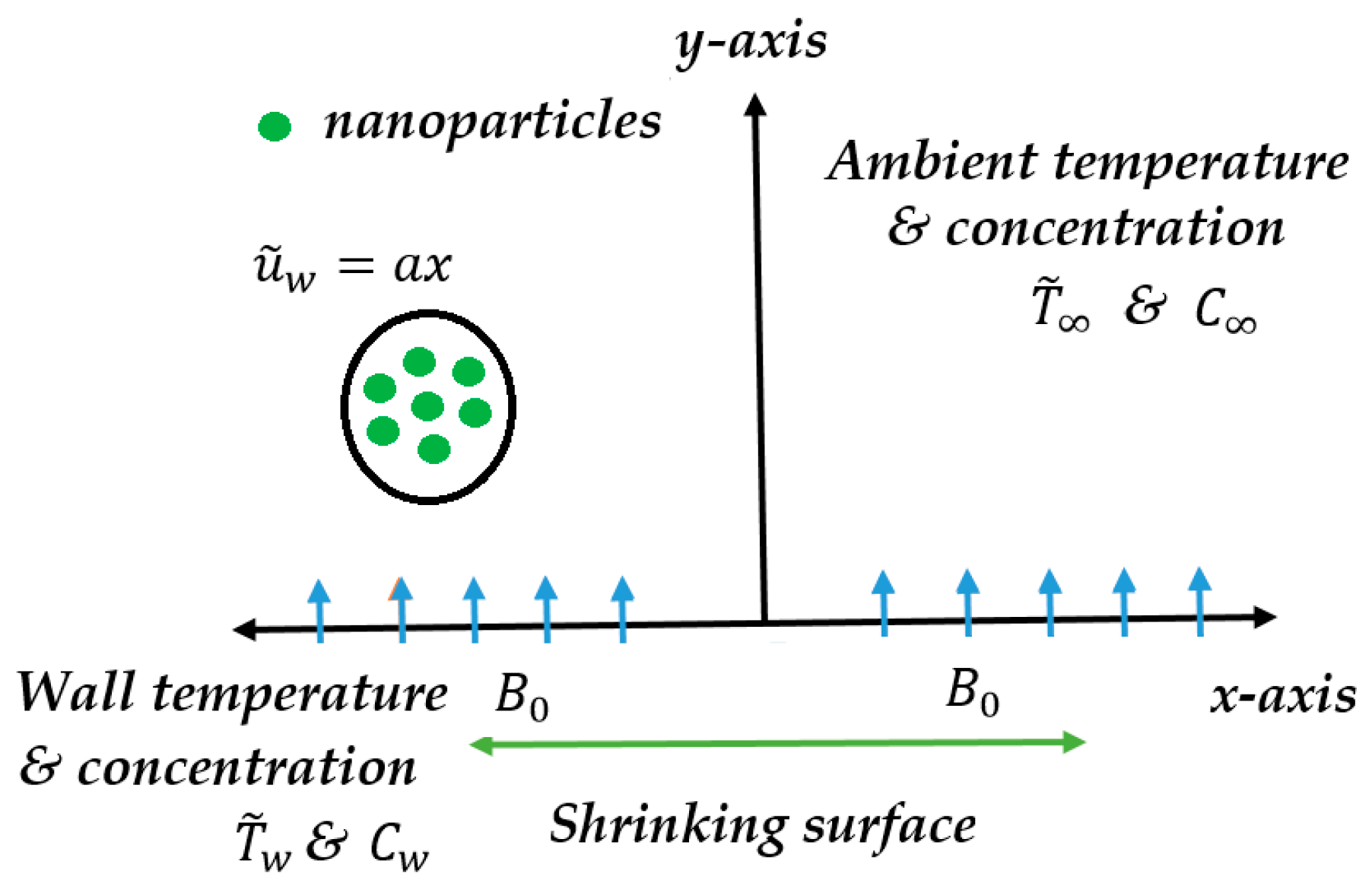
2. Mathematical Formulation

Let us consider the MHD boundary layer flow of a Carreau nanofluid over a shrinking surface near a stagnation point at$y=0$. The MHD flow occurs in the domain at $y>0$. The fluid is electrically conducting by an external magnetic field while the induced magnetic is assumed to be zero. Cartesian coordinate is chosen in a way such that $x-$axis is considered along the direction of the sheet whereas $y-$axis is considered along normal to it as shown in Figure 1. Suppose that ${\tilde{T}}_w$ and $C_w$ be the temperature and the nano particle fraction at the sheet while the temperature and nano-particle fraction at infinity is ${\tilde{T}}_{\infty }$and$C_{\infty }$.

The governing equations of Carreau nanofluid model can be written as [26]:

$$\frac{\partial \tilde{u}}{\partial x}+\frac{\partial \tilde{v}}{\partial y}=0,$$

(1)

$$\tilde{u}\frac{\partial \tilde{u}}{\partial x}+\tilde{v}\frac{\partial \tilde{v}}{\partial y}=\nu \frac{{\partial }^2\tilde{u}}{\partial y^2}+{\tilde{u}}_e\frac{d{\tilde{u}}_e}{dx}+\frac{3\left(n-1\right)\nu {\overline{\Gamma }}^2}{2}{\left(\frac{\partial \tilde{u}}{\partial y}\right)}^2\frac{{\partial }^2\tilde{u}}{\partial y^2} +\frac{\sigma B_0^2}{\rho }\left({\tilde{u}}_e-\tilde{u}\right),$$

(2)

$$\tilde{u}\frac{\partial \tilde{T}}{\partial x}+\tilde{v}\frac{\partial \tilde{T}}{\partial y}=\overline{\alpha }\frac{{\partial }^2\tilde{T}}{\partial y^2} +\tau \left(D_B\frac{\partial C}{\partial y}\frac{\partial \tilde{T}}{\partial y}+\frac{D_T}{T_{\infty }}{\left(\frac{\partial \tilde{T}}{\partial y}\right)}^2\right)-\frac{1}{\rho c_p}\frac{\partial q_r}{\partial y},$$

(3)

$$\tilde{u}\frac{\partial C}{\partial x}+\tilde{v}\frac{\partial C}{\partial y}=D_B\frac{{\partial }^{2}C}{\partial y^2}+\frac{D_T}{T_{\infty }}\frac{{\partial }^2\tilde{T}}{\partial y^2}.$$

(4)

Taking the approximation of Rosseland for radiation, the radiative heat flux $q_r$ is defined as:

$$q_r=-\frac{4\overline{\sigma }}{3\overline{k}}\frac{\partial {\tilde{T}}^4}{\partial y}.$$

(5)

Let us consider that temperature with in the nano particles is very small such that the term $T^4$ can be expanded about a free stream temperature $T_0$ as:

$${\tilde{T}}^4={\tilde{T}}_0^4+4{\tilde{T}}_0^3\left(\tilde{T}-{\tilde{T}}_0\right)+6{\tilde{T}}_0^2{\left(\tilde{T}-{\tilde{T}}_0\right)}^2+\dots .$$

(6)

After neglecting the higher order terms in the above equation, it can be written as:

$${\tilde{T}}^4\cong 4{\tilde{T}}_0^3\left(\tilde{T}-{\tilde{T}}_0\right).$$

(7)

With the help of Equations (5)–(7), the nonlinear radiative heat flux can be written as:

$$q_r=-\frac{4\overline{\sigma }}{3\overline{k}} \frac{\partial {\tilde{T}}^4}{\partial y}=-\frac{16\overline{\sigma }{\tilde{T}}^3}{3\overline{k}}\frac{\partial \tilde{T}}{\partial y},$$

(8)

and their respective boundary conditions are:

$$\tilde{u}=u_w, \tilde{v}={\tilde{v}}_w, \tilde{T}={\tilde{T}}_w, C=C_w \text{at }y=0,$$

(9)

$$\tilde{u}={\tilde{u}}_e, \tilde{v}=0, \tilde{T}\to {\tilde{T}}_{\infty }, C\to C_{\infty } \text{as }y\to \infty .$$

(10)

The steam function satisfying Equation (1) are defined as $\tilde{u}=\partial \phi /\partial y$ and $\tilde{v}=-\partial \phi /\partial x$. The velocity of the sheet is considered along $x-$axis i.e., ${\tilde{u}}_w=ax$. Defining the following similarity transformation variables:

$$\zeta =\sqrt{\frac{{\tilde{u}}_w}{\nu x} }y, \tilde{u}={\tilde{u}}_w{f}^{\prime }\left(\zeta \right),\tilde{v}=-\sqrt{\frac{\nu {\tilde{u}}_w}{x}}f\left(\zeta \right), \theta =\frac{\tilde{T}-{\tilde{T}}_{\infty } }{{\tilde{T}}_w-{\tilde{T}}_{\infty }}, \varphi =\frac{C-C_{\infty } }{C_w-C_{\infty }},$$

(11)

and using Equation (8) in to Equations (7) and (3), we get:

$$f^{\prime \prime \prime }+1+\frac{3\left(n-1\right)W{e}^2}{2}{f}^{\prime \prime 2}f\prime \prime \prime -f^{\prime 2}+f{f}^{″}+M\left(1-f^{\prime }\right)=0,$$

(12)

$$\left(\frac{1}{{\mathrm{P}}_{\mathrm{r}}}+N_r\right){\theta }^{\prime \prime }+f{\theta }^{\prime }+N_b{\theta }^{\prime }{\varphi }^{\prime }+N_t{\left({\theta }^{\prime }\right)}^2=0,$$

(13)

$${\varphi }^{″}+L_{e}f{\varphi }^{\prime }+\frac{N_t}{N_b}{\theta }^{″}=0.$$

(14)

In the above equations, for $n=1,$the present study can be reduced to Newtonian fluid, whereas for $n>1,$the mechanism remains non-Newtonian fluid. Their corresponding boundary conditions are:

$$f\left(0\right)=S, f^{\prime }\left(0\right)=\alpha , f^{\prime }\left(\infty \right)=1,$$

(15)

$$\theta \left(0\right)=1, \theta \left(\infty \right)=0,$$

(16)

$$\varphi \left(0\right)=1,\varphi \left(\infty \right)=0,$$

(17)

where ${\mathrm{P}}_{\mathrm{r}}=\nu /\overline{\alpha }$, $M=B_0^2\sigma /c\rho$, $L_e=\frac{\nu }{D_B}, N_b=\frac{\tau D_B\left({\varphi }_w-{\varphi }_{\infty }\right)}{\nu }, N_t=\frac{\tau D_T\left({\tilde{T}}_w-{\tilde{T}}_{\infty }\right)}{{\tilde{T}}_{\infty }\nu },N_r=\frac{16\overline{\sigma }{\tilde{T}}^3}{3\rho c_p\overline{k}} .$

3. Physical Quantities of Interest

The physical quantities of interest for the governing flow problem are local Nusselt number and local Sherwood number which can be written as:

$$N{u}_x=\frac{x{q}_w}{\kappa \left({\tilde{T}}_w-{\tilde{T}}_{\infty }\right)}, S{h}_x=\frac{x{q}_m}{D_B\left(C_w-C_{\infty }\right)}$$

(18)

where $q_w$ and $q_m$ are described as:

$$q_w= -\kappa {\left(\frac{\partial \tilde{T}}{\partial y}\right)}_{y=0}, q_m=D_B{\left(-\frac{\partial C}{\partial y}\right)}_{y=0}.$$

(19)

With the help of dimensionless transformation in Equation (11), we have:

$$N{u}_r=\frac{N{u}_x}{{\text{Re}}_x^{\frac{1}{2}}}= -\left(1+N_r\right){\theta }^{\prime }\left(0\right), S{h}_r=\frac{S{h}_x}{{\text{Re}}_x^{\frac{1}{2}}}=-{\varphi }^{\prime }\left(0\right),$$

(20)

where $S{h}_r$ and $N{u}_r$are the dimensionless Sherwood number and local Nusselt number, respectively, and ${\text{Re}}_x={\tilde{u}}_{w}x/\nu$ is the local Reynolds number.

4. Numerical Method

We apply the Successive linearization method to Equation (12) with their boundary conditions in Equation (15), by setting [35]:

$$f\left(\zeta \right)=f_I\left(\zeta \right)+{\displaystyle \sum }_{N=0}^{I-1}{f}_N\left(\zeta \right), \left(I=1,2,3,\dots \right),$$

(21)

where $f_I$are unknown functions which are obtained by iteratively solving the linearized version of the governing equation and assuming that $f_I \left(0\le N\le I-1\right)$ are known from previous iterations. Our algorithm starts with an initial approximation $f_0$ which satisfy the given boundary conditions in Equation (16) according to SLM. The suitable initial guess for the governing flow problem is:

$$f_0=-1+\zeta +\alpha +S+\frac{1-\alpha }{e^{\zeta }}.$$

(22)

We write the equation in general form as:

$$L\left(f,f^{\prime },f^{″},f^{‴}\right)+N\left(f,f^{\prime },f^{″},f^{‴}\right)=0,$$

(23)

where:

$$L\left(f,f^{\prime },f^{″},f^{‴}\right)=f^{‴},$$

(24)

and:

$$N\left(f,f^{\prime },f^{″},f^{‴}\right)=f{f}^{″}+1-f^{\prime 2}+M\left(1-f^{\prime }\right)+\frac{3\left(n-1\right)W{e}^2}{2}{f}^{\prime \prime 2}f\prime \prime \prime ,$$

(25)

where $L$ and $N$ are the linear and non-linear part of Equation (12). By substituting Equation (21) in Equation (12) and taking the linear terms only, we get:

$$f_I^{\prime \prime \prime }+A_{0,I-1}{f}_I^{\prime \prime }+A_{1,I-1}{f}_I^{\prime }+A_{2,I-1}{f}_I=r_{I-1},$$

(26)

the corresponding boundary conditions becomes:

$$f_I\left(0\right)=0, f_I^{\prime }\left(0\right)=0,f_I^{\prime }\left(\infty \right)=0.$$

(27)

We solve Equation (26) numerically by a well-known method, namely, the Chebyshev spectral collocation method. For numerical implementation, the physical region $\left[0,\infty \right)$is truncated to $\left[0,\mathsf{\Gamma }\right]$ we can take $\mathsf{\Gamma }$ to be sufficiently large. With the help of following transformations this region is further transformed in to$\left[-1,1\right]$, we have:

$$\mathsf{\Omega }=-1+\frac{2\zeta }{\mathsf{\Gamma }}.$$

(28)

We define the following discretization between the interval$\left[-1,1\right]$. Now, we can apply Gause-Lobatto collocation points to define the nodes between $\left[-1,1\right]$ by:

$${\mathsf{\Omega }}_J=\cos \frac{\pi J}{N}, \left(J=0,1,2,3\dots N\right),$$

(29)

with $\left(N+1\right)$ number of collocation points. Chebyshev spectral collocation method based on the concept of differentiation matrix$D$. This differentiation matrix maps a vector of the function values the collocation points to a vector $G^{\prime }$ is defined as:

$$G^{\prime }={\displaystyle \sum }_{K-0}^N{D}_{KJ}f\left({\mathsf{\Omega }}_K\right)=DG,$$

(30)

the derivative of$p$order for the function $f\left(\mathsf{\Omega }\right)$ can be written as:

$$f^p\left(\mathsf{\Omega }\right)=D^{p}G.$$

(31)

The entries of matrix $D$can be computed by the method proposed by Bhatti et al. [39]. Now, applying the spectral method, with derivative matrices on linearized equation Equations (26) and (27), we get the following linearized matrix system

$$A_{I-1}{G}_I=R_{I-1},$$

(32)

the boundary conditions takes the following form:

$$f_I\left({\mathsf{\Omega }}_N\right)=0, {\displaystyle \sum }_{K=0}^N{D}_{NK}{f}_I\left({\mathsf{\Omega }}_K\right)=0,{\displaystyle \sum }_{K=0}^N{D}_{0K}{f}_I\left({\mathsf{\Omega }}_K\right)=0,{\displaystyle \sum }_{K=0}^N{D}_{0K}^2{f}_I\left({\mathsf{\Omega }}_K\right)=0,$$

(33)

where:

$$A_{I-1}=D^3+A_{0,I-1}{D}^2+A_{1,I-1}D+A_{2,I-1}.$$

(34)

In the above equation $A_{s,I-1}\left(s=0,1,\dots 3\right)$ are $\left(N+1\right)\times \left(N+1\right)$ diagonal matrices with $A_{s,I-1}\left({\mathsf{\Omega }}_J\right)$ on the main diagonal and:

$$G_I=f_I\left({\mathsf{\Omega }}_J\right), R_I=r_I\left({\mathsf{\Omega }}_J\right). \left(J=0,1,2,3,\dots N\right).$$

(35)

After employing Equation (31) on the solutions for $f_I$ are obtained by solving iteratively Equation (33). We obtain the solution for $f\left(\zeta \right)$ from solving Equation (34) and now Equations (13) and (14) are now linear therefore, we will apply Chebyshev pseudo-spectral method directly, we get:

$$BH=S,$$

(36)

with their corresponding boundary conditions boundary conditions:

$$\theta \left({\mathsf{\Omega }}_N\right)=1,\theta \left({\mathsf{\Omega }}_0\right)=0,$$

(37)

$$\varphi \left({\mathsf{\Omega }}_N\right)=1,\varphi \left({\mathsf{\Omega }}_0\right)=0,$$

(38)

where $H=\left(\theta \left({\mathsf{\Omega }}_J\right),\varphi \left({\mathsf{\Omega }}_J\right)\right),$ $B$is the set of linear coupled equation of temperature and nanoparticle concentration, $S$ is a vector of zeros, and all vectors in Equation (36) are converted to diagonal matrix. We imposed the boundary conditions in Equations (37) and (38) on the first and last rows of $B$ and $S$, respectively.

5. Entropy Generation Analysis

The volumetric entropy generation of the Williamson nanofluid is given by [26]:

$$S_{gen}^{\prime \prime \prime }=\frac{\kappa }{{\tilde{T}}_{\infty }^2}\left[{\left(\frac{\partial \tilde{T}}{\partial y}\right)}^2+\frac{16\overline{\sigma }{\tilde{T}}^3}{3\overline{k}}{\left(\frac{\partial \tilde{T}}{\partial y}\right)}^2\right]+\frac{\mu }{{\tilde{T}}_{\infty }}\left({\left(\frac{\partial \tilde{u}}{\partial \tilde{y}}\right)}^2+\frac{\left(n-1\right)\nu {\overline{\mathsf{\Gamma }}}^2}{2}{\left(\frac{\partial \tilde{u}}{\partial y}\right)}^4\right)+\frac{RD}{C_{\infty }}{\left(\frac{\partial C}{\partial y}\right)}^2+\frac{\sigma B_0^2}{{\tilde{T}}_{\infty }}{\tilde{u}}^2+\frac{RD}{{\tilde{T}}_{\infty }}\left(\frac{\partial \tilde{T}}{\partial y}\frac{\partial C}{\partial y}+\frac{\partial C}{\partial x}\frac{\partial \tilde{T}}{\partial x}\right).$$

(39)

In the above equation, the entropy generation consists of three effects, (i) conduction effect (also known as heat transfer irreversibility, (HTI)); (ii) fluid friction irreversibility (FFI) and (iii) diffusion (also known as diffusive irreversibility, (DI)). The characteristics entropy generation can be written as:

$$S_0^{\prime \prime \prime }=\frac{\kappa {\left(\mathsf{\Delta }T\right)}^2}{L^2{\tilde{T}}_{\infty }^2 }.$$

(40)

With the help of Equation (8), the entropy generation in dimensionless form can be written as:

$$N_G=\frac{S_{gen}^{\prime \prime \prime }}{S_0^{\prime \prime \prime }}=\text{Re}\left(1+N_r\right){\theta }^{\prime 2}\left(\zeta \right)+\frac{\text{Re}{B}_r}{\mathsf{\Omega }}\left(f^{\prime \prime 2}\left(\zeta \right)+\frac{\left(n-1\right)\nu W{e}^2}{2}{f}^{\prime \prime 4}\left(\zeta \right)\right)+\frac{\text{Re}{B}_r}{\mathsf{\Omega }}M{f}^{\prime 2}\left(\zeta \right)+\text{Re}{\lambda }_1{\left(\frac{\chi }{\mathsf{\Omega }}\right)}^2{\varphi }^{\prime 2}\left(\zeta \right)+\text{Re}{\lambda }_1\left(\frac{\chi }{\mathsf{\Omega }}\right){\theta }^{\prime }\left(\zeta \right){\varphi }^{\prime }\left(\zeta \right).$$

(41)

These number are given in the following form:

$$\text{Re}=\frac{{\tilde{u}}_L{L}^2}{\nu }, B_r=\frac{\mu {\tilde{u}}_w{}^2}{\kappa \mathsf{\Delta }T}, \mathsf{\Omega }=\frac{\mathsf{\Delta }T}{{\tilde{T}}_{\infty }}, \chi =\frac{\mathsf{\Delta }C}{C_{\infty }}, {\lambda }_1=\frac{RD{C}_{\infty }}{\kappa }.$$

(42)

6. Results and Discussions

In this section, we will discuss the behavior of various emerging parameters with the help of table and graphics. The graphical results are sketched for velocity profile, temperature profile, concentration profile, and entropy profile against Hartmann number, thermophoresis parameter, Brownian motion parameter, Lewis number, fluid parameter, radiation parameter, Reynolds number, Brinkmann number, and Prandtl number, respectively. Furthermore, the present study can be reduced to Newtonian fluid also, by taking $n=1,$or$We=0$.

Table 1. Numerical values of reduced Nusselt number $\left(N{u}_r\right)$ and Sherwood number $\left(S{h}_r\right)$ for various values of$\text{Pr}, N_r, N_b, \text{and }{N}_t$.

$Pr$	$N_r$	$N_b$	$N_t$	$L_e$	$N{u}_r$	$S{h}_r$
$1$	$0.5$	$0.2$	$0.2$	$1$	$1.6734$	-
$2$	-	-	-	-	2.1657	-
$10$	-	-	-	-	2.9205	-
-	$1$	-	-	-	1.8475	-
-	$2$	-	-	-	$2.1193$	-
-	$3$	-	-	-	$2.3387$	-
-	-	$0.1$	-	-	$1.7499$	0.7765
-	-	$0.3$	-	-	$1.6044$	1.2441
-	-	$0.6$	-	-	1.4333	1.5063
-	-	-	$0.1$	-	$1.7499$	1.3605
-	-	-	$0.3$	-	$1.6044$	0.8944
-	-	-	$0.6$	-	1.4333	0.6264
-	-	-	-	$1.5$	-	1.5063
-	-	-	-	$2$	-	1.9470
-	-	-	-	$3$	-	2.8467

shows the numerical values of local Nusselt number and local Sherwood number for different values of all the physical parameters.

Table 2. Comparison of $f^{″}\left(0\right)$ with existing published results for $M=0$ and $n=1, We=0$.

$\alpha$	Present Results	Bhatti et al. [39] $\left(k\to 0\right)$	Mahapatra and Nandy [40]	Lok et al. [41]	Wang [42]
$0.0$.	$1.2325$	$1.2325$	$1.2325$	-	$1.2325$
$0.5$	$0.7133$	$0.7133$	$0.7133$	$0.7133$	$0.7133$
$1.0$	$0$	$0$	$0$	$0$	$0$
$2.0$	$-1.8873$	$-1.8873$	$-1.8873$	$-1.8873$	$-1.8873$
$-0.5$	$1.4956$	$1.4956$	$1.4956$	-	$1.4956$.
$-1.0$	$1.3288$	$1.3288$	$1.3288$	-	$1.3288$
$-1.15$	$1.0822$	$1.0822$	$1.0822$	-	$1.0822$

shows the numerical comparison with existing published results by taking $n=1, We=0$ (Newtonian fluid) and $M=0$ as special case of our study. We can observe from Table 1 that the present results are in very good agreement with the existing published data. Figure 2 is plotted for velocity profile against Hartmann number $\left(M\right)$ and Weissenberg number$\left(We\right)$. From this figure, we can observe that velocity profile diminish due to the increment in Weissenberg number. However, we can also observe that velocity depicts similar behavior when the influence of magnetic field increases. In fact, it happens due to the influence of Lorentz force which provides resistance and opposes the flow. It depicts from Figure 3 that when the power law index $\left(n\right)$ increases it tends to reduce the velocity profile. One more interesting thing, we observe that when the fluid depicts non-Newtonian behavior then the profile decreases as compared to Newtonian behavior of the fluid.

Figure 4 and Figure 5 present the temperature profiles for different values of Prandtl numbers, thermophoresis parameter, Brownian motion parameter and radiation parameter. It can be noticed from Figure 4 that when the thermophoresis parameter $\left(N_t\right)$increases then the temperature profile also enhances and also the boundary layer thickness increases, however the behavior of temperature profile remains same when the Brownian motion parameter increases$\left(N_b\right)$. Physically, an increment in thermophoresis parameter creates a force which leads to move the nanoparticles from hotter region to the colder region which in results enhances the temperature and the boundary layer thickness increases. From Figure 5 we can analyze that with the increment in radiation parameter$\left(N_r\right)$, temperature profile increases and its attitude is completely opposite with the increment in Prandtl number. Moreover, we can also observe that for large values of Prandtl number$\left(P_r\right)$, momentum diffusivity is more dominating as compared to thermal diffusivity. Figure 6 and Figure 7 are sketched from the concentration profile against, Brownian motion parameter, thermophoresis parameter and Prandtl number. It can be observed from Figure 6 that thermophoresis parameter $\left(N_t\right)$ enhances the concentration profile, but Brownian motion parameter $\left(N_b\right)$provides resistance to the concentration profile and as a result concentration profile and boundary layer thickness increases. It can be examined from Figure 7 that with the increment in Lewis number$\left(L_e\right)$, nanoparticle concentration profiles diminish and its associated boundary layer thickness. Figure 8, Figure 9, Figure 10 and Figure 11 are drawn for the entropy profile for all of the physical parameters of interest. From Figure 8, Figure 9 and Figure 10 we can see that entropy profile decreases initially, but it starts changing its behavior after certain values of $\left(\zeta >0.5\right).$From Figure 11, we can analyze that the Reynolds number $\left(\text{Re}\right)$ enhances the entropy profile.

7. Conclusions

In this article, entropy generation with thermal radiation on a Carreau nanofluid towards a shrinking sheet has been investigated numerically under the influence of magnetohydrodynamics (MHD). The governing flow problem is modeled using Ohms law and with the help of momentum, thermal energy, and nanoparticle concentration equations. The resulting partial differential equations are simplified into ordinary differential equations using similarity transformation variables. Numerical computation has been employed with the combination of the successive linearization method and Chebyshev spectral collocation method. The main observations for the present flow problem are described below:

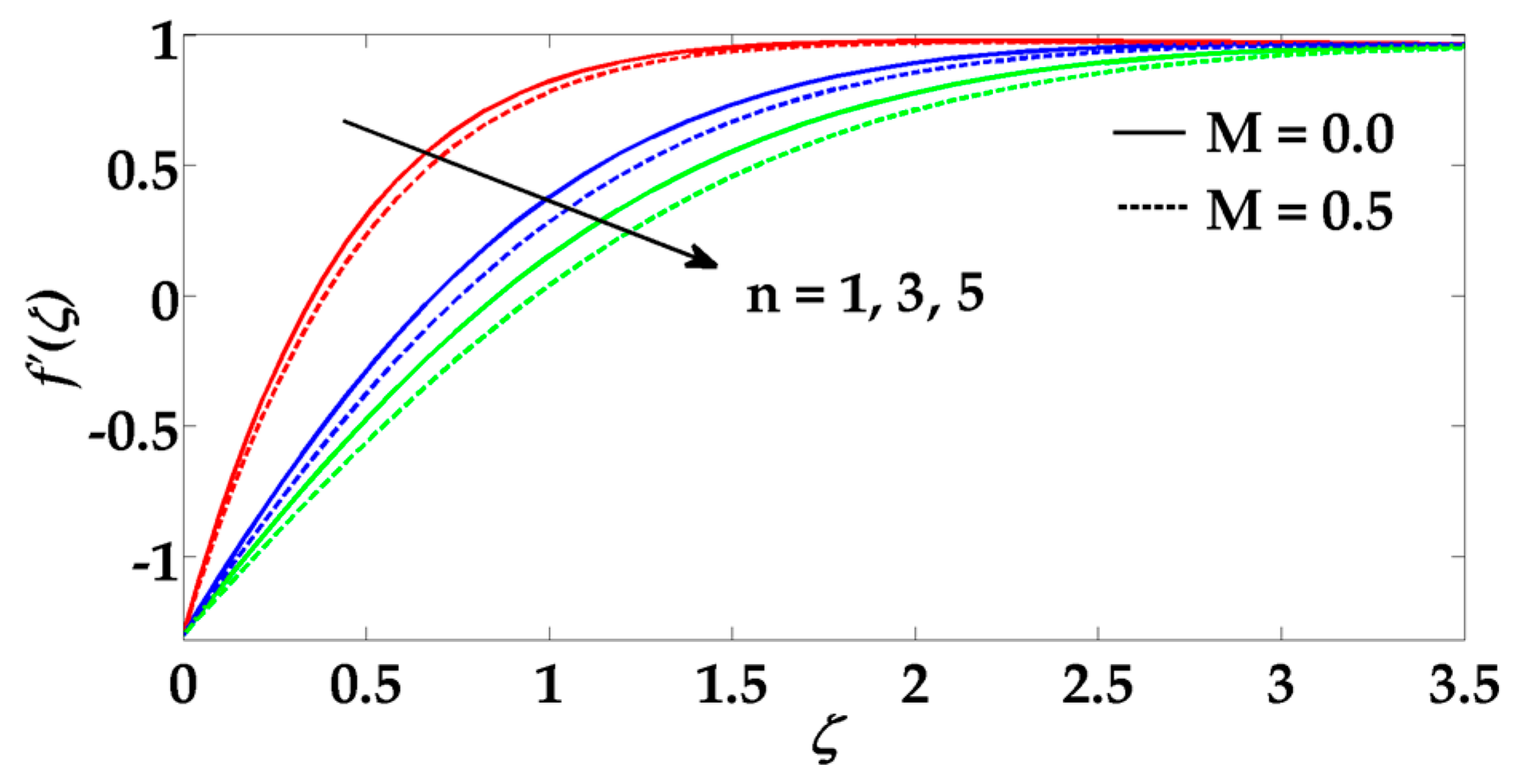
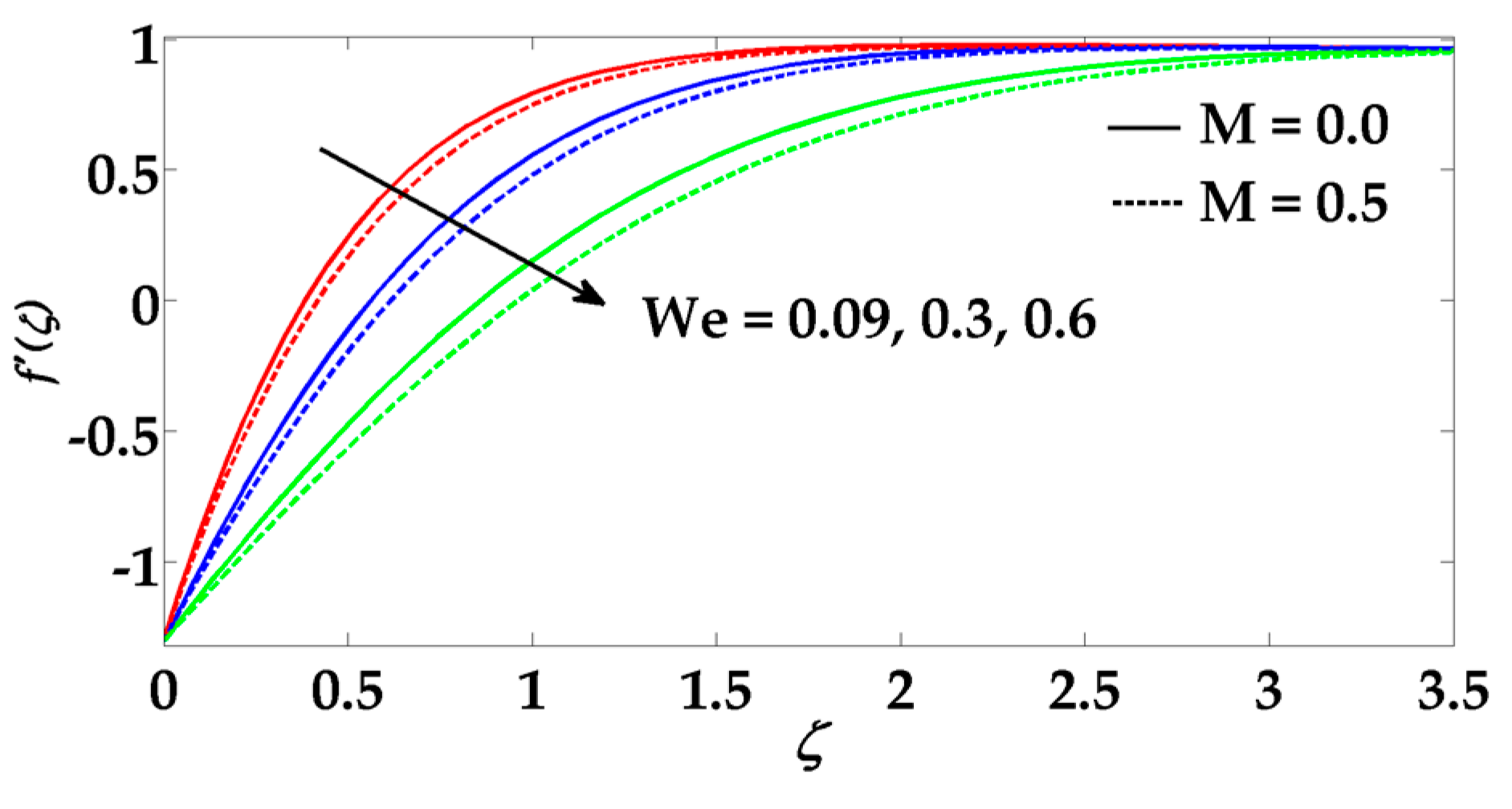
• The magnitude of the velocity decreases for larger values of Hartmann numbers and fluid parameters.
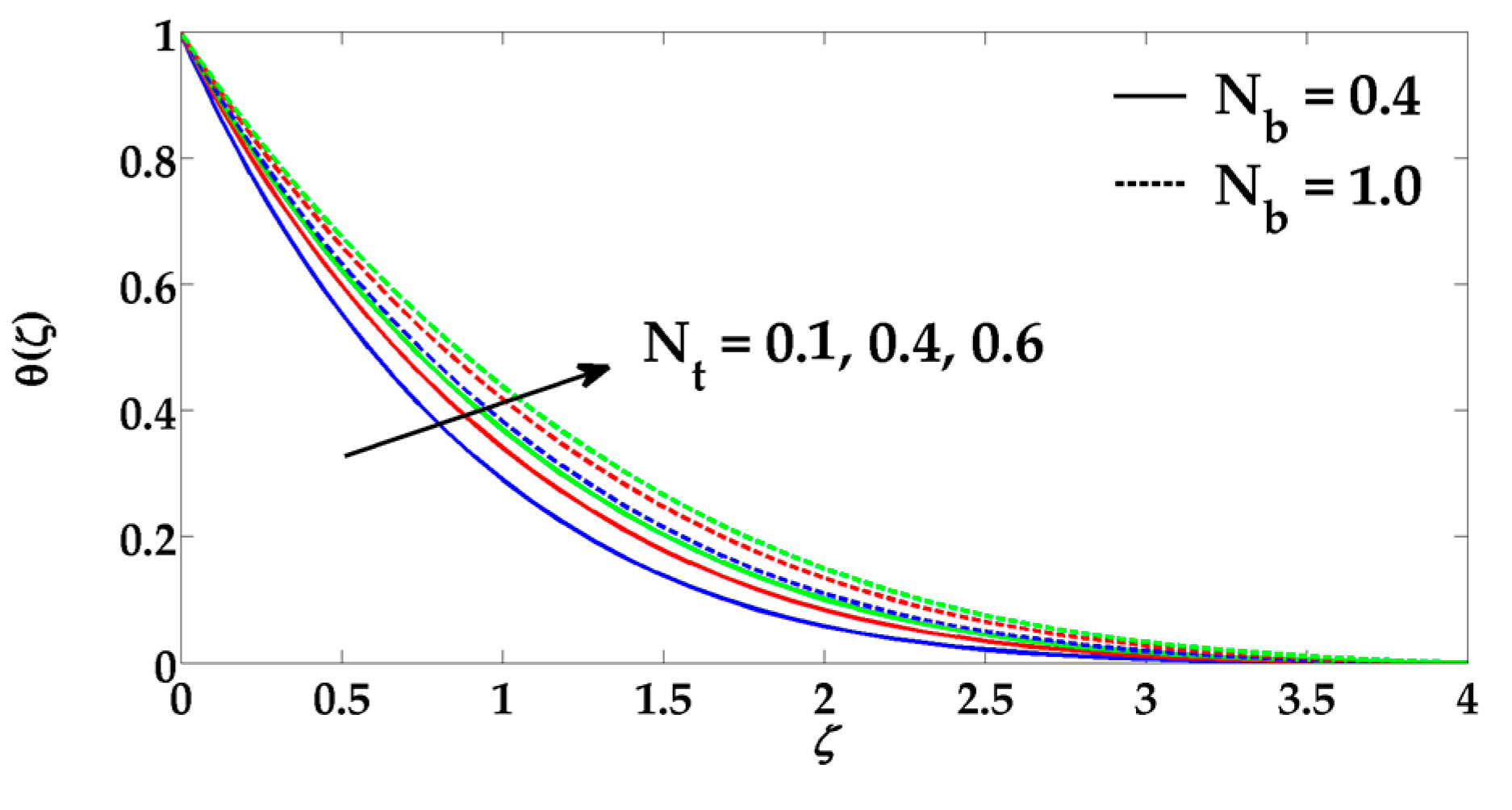
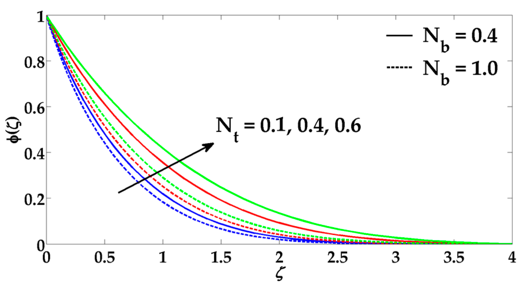
• The Brownian motion parameter and thermophoresis parameter show similar behavior on the temperature profile.
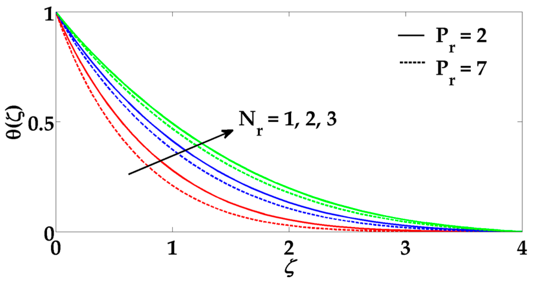
• Larger values of the thermal radiation parameter enhance the temperature profile.
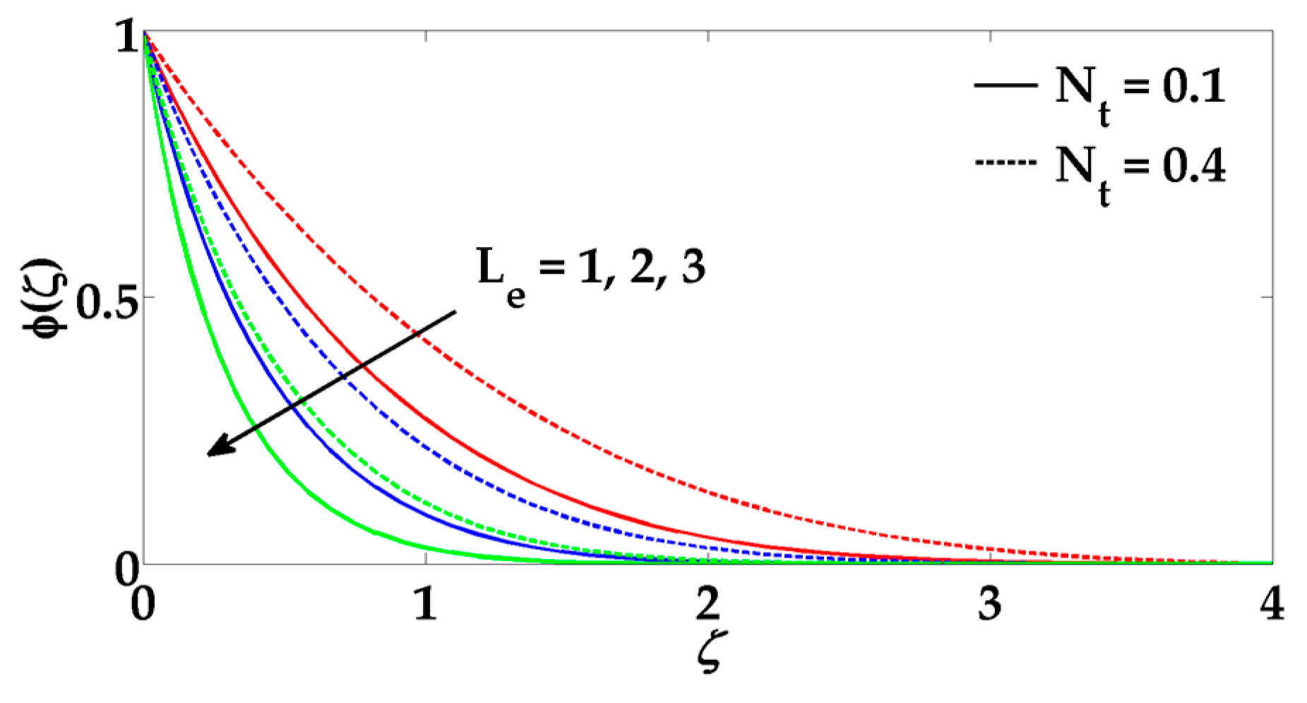
• The concentration profile also behaves as a decreasing function due to the increment in the Lewis number.
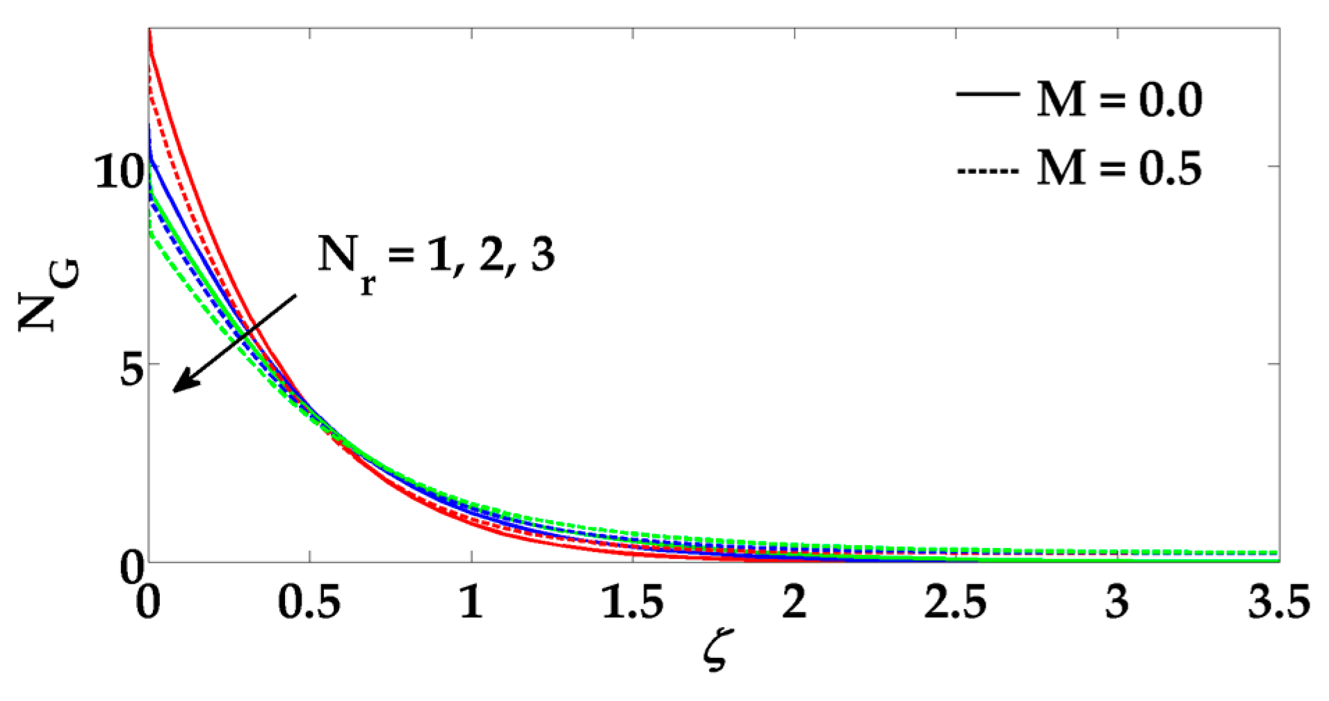
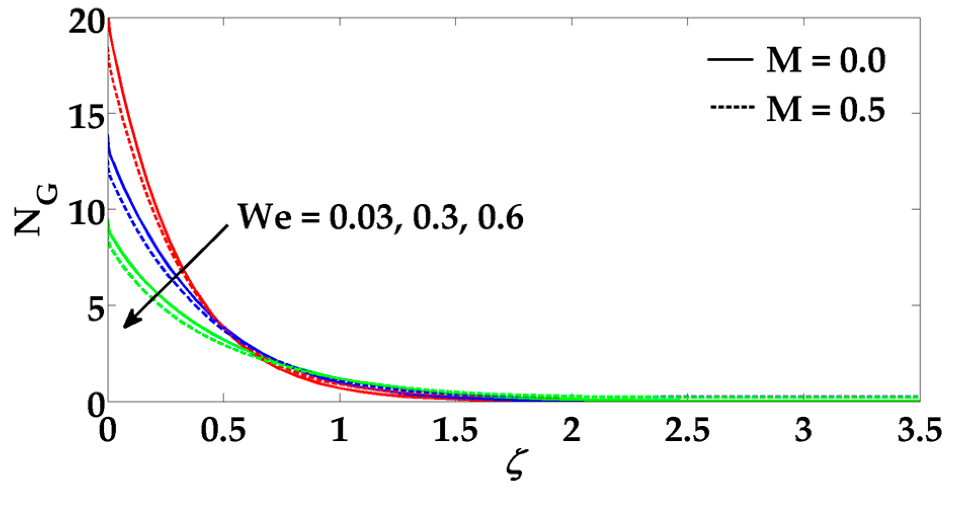
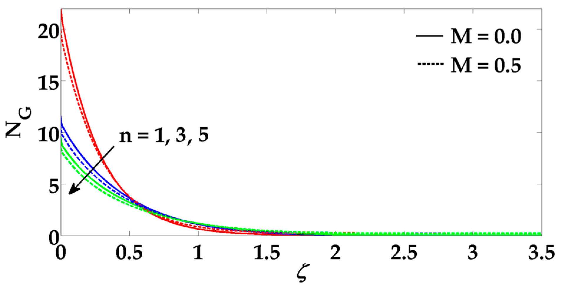
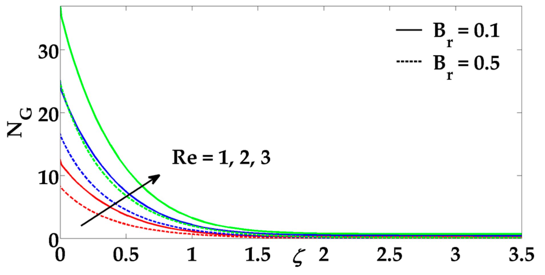
• The entropy profile behaves as an increasing function of all the physical parameters of interest.

References

1. Saidur, R.; Leong, K.Y.; Mohammad, H.A. A review on applications and challenges of nanofluids. Renew. Sustain. Energy Rev. 2011, 15, 1646–1668. [Google Scholar] [CrossRef]
2. Liu, Z.H.; Li, Y.Y. A new frontier of nanofluid research–application of nanofluids in heat pipes. Int. J. Heat Mass Transf. 2012, 55, 6786–6797. [Google Scholar] [CrossRef]
3. Akbar, N.S.; Khan, Z.H. Magnetic field analysis in a suspension of gyrotactic microorganisms and nanoparticles over a stretching surface. J. Magn. Magn. Mater. 2016, 410, 72–80. [Google Scholar] [CrossRef]
4. Hayat, T.; Imtiaz, M.; Alsaedi, A. Unsteady flow of nanofluid with double stratification and magnetohydrodynamics. Int. J. Heat Mass Transf. 2016, 92, 100–109. [Google Scholar] [CrossRef]
5. Ellahi, R.; Hassan, M.; Zeeshan, A. Study of natural convection MHD nanofluid by means of single and multi-walled carbon nanotubes suspended in a salt-water solution. IEEE Trans. Nanotechnol. 2015, 14, 726–734. [Google Scholar] [CrossRef]
6. Ellahi, R.; Hassan, M.; Zeeshan, A.; Khan, A.A. The shape effects of nanoparticles suspended in HFE-7100 over wedge with entropy generation and mixed convection. Appl. Nanosci. 2015, 1–11. [Google Scholar] [CrossRef]
7. Garoosi, F.; Hoseininejad, F.; Rashidi, M.M. Numerical study of heat transfer performance of nanofluids in a heat exchanger. Appl. Thermal Eng. 2016. [Google Scholar] [CrossRef]
8. Ali, M.; Zeitoun, O.; Almotairi, S. Natural convection heat transfer inside vertical circular enclosure filled with water-based Al2O3 nanofluids. Int. J. Therm. Sci. 2013, 63, 115–124. [Google Scholar] [CrossRef]
9. Ali, M.; Zeitoun, O.; Almotairi, S.; Al-Ansary, H. The effect of Alumina-water nanofluid on natural convection heat transfer inside vertical circular enclosure heated from above. Heat Transf. Eng. 2013, 34, 1289–1299. [Google Scholar] [CrossRef]
10. Zeitoun, O.; Ali, M. Nanofluid impingement jet heat transfer. Nanoscale Res. Lett. 2012, 7, 139. [Google Scholar] [CrossRef] [PubMed]
11. Zeitoun, O.; Ali, M.; Al-Ansary, H. The effect of particle concentration on cooling of a circular horizontal surface using nanofluid jets. Nanoscale Microscale Thermophys. Eng. 2013, 17, 154–171. [Google Scholar] [CrossRef]
12. Ali, M; Zeitoun, O. Nanofluids forced convection heat transfer inside circular tubes. Int. J. Nanopart. 2009, 2, 164–172. [Google Scholar]
13. Murshed, S.M.S.; Leong, K.C.; Yang, C. Thermophysical and electrokinetic properties of nanofluids—A critical review. Appl. Thermal Eng. 2008, 28, 2109–2125. [Google Scholar] [CrossRef]
14. Scherer, C.; Figueiredo Neto, A.M. Ferrofluids: Properties and applications. Braz. J. Phys. 2005, 35, 718–727. [Google Scholar] [CrossRef]
15. Baumgartl, J.; Hubert, A.; Müller, G. The use of magnetohydrodynamic effects to investigate fluid flow in electrically conducting melts. Phys. Fluids A Fluid Dyn. (1989–1993) 1993, 5, 3280–3289. [Google Scholar] [CrossRef]
16. Rashidi, M.M.; Keimanesh, M.; Bég, O.A.; Hung, T.K. Magnetohydrodynamic biorheological transport phenomena in a porous medium: A simulation of magnetic blood flow control and filtration. Int. J. Numer. Methods Biomed. Eng. 2011, 27, 805–821. [Google Scholar] [CrossRef]
17. Nisar, A.; Afzulpurkar, N.; Mahaisavariya, B.; Tuantranont, A. MEMS-based micropumps in drug delivery and biomedical applications. Sens. Actuators B Chem. 2008, 130, 917–942. [Google Scholar] [CrossRef]
18. Mabood, F.; Ibrahim, S.M.; Rashidi, M.M.; Shadloo, M.S.; Lorenzini, G. Non-uniform heat source/sink and Soret effects on MHD non-Darcian convective flow past a stretching sheet in a micropolar fluid with radiation. Int. J. Heat Mass Transf. 2016, 93, 674–682. [Google Scholar] [CrossRef]
19. Rashidi, M.M.; Rostami, B.; Freidoonimehr, N.; Abbasbandy, S. Free convective heat and mass transfer for MHD fluid flow over a permeable vertical stretching sheet in the presence of the radiation and buoyancy effects. Ain Shams Eng. J. 2014, 5, 901–912. [Google Scholar] [CrossRef]
20. Zeeshan, A.; Majeed, A.; Ellahi, R. Effect of magnetic dipole on viscous ferro-fluid past a stretching surface with thermal radiation. J. Mol. Liq. 2016, 215, 549–554. [Google Scholar] [CrossRef]
21. Yasin, M.H.M.; Ishak, A.; Pop, I. MHD heat and mass transfer flow over a permeable stretching/shrinking sheet with radiation effect. J. Magn. Magn. Mater. 2016, 407, 235–240. [Google Scholar] [CrossRef]
22. Mabood, F.; Khan, W.A. Analytical study for unsteady nanofluid MHD Flow impinging on heated stretching sheet. J. Mol. Liq. 2016, 219, 216–223. [Google Scholar] [CrossRef]
23. Sandeep, N.; Sulochana, C.; Kumar, B.R. Unsteady MHD radiative flow and heat transfer of a dusty nanofluid over an exponentially stretching surface. Eng. Sci. Technol. Int. J. 2016, 19, 227–240. [Google Scholar] [CrossRef]
24. Ene, R.D.; Marinca, V. Approximate solutions for steady boundary layer MHD viscous flow and radiative heat transfer over an exponentially porous stretching sheet. Appl. Math. Comput. 2015, 269, 389–401. [Google Scholar] [CrossRef]
25. Rashidi, M.M.; Kavyani, N.; Abelman, S. Investigation of entropy generation in MHD and slip flow over a rotating porous disk with variable properties. Int. J. Heat Mass Transf. 2014, 70, 892–917. [Google Scholar] [CrossRef]
26. Qing, J.; Bhatti, M.M.; Abbas, M.A.; Rashidi, M.M.; Ali, M.E.-S. Entropy Generation on MHD Casson Nanofluid Flow over a Porous Stretching/Shrinking Surface. Entropy 2016, 18, 1–14. [Google Scholar] [CrossRef]
27. Mahmud, S.; Fraser, R.A. Magnetohydrodynamic free convection and entropy generation in a square porous cavity. Int. J. Heat Mass Transf. 2004, 47, 3245–3256. [Google Scholar] [CrossRef]
28. Tasnim, S.H.; Shohel, M.; Mamun, M.A.H. Entropy generation in a porous channel with hydromagnetic effect. Exergy 2002, 2, 300–308. [Google Scholar] [CrossRef]
29. Butt, A.S.; Ali, A. Entropy effects in hydromagnetic free convection flow past a vertical plate embedded in a porous medium in the presence of thermal radiation. Eur. Phys. J. Plus 2013, 128, 51–65. [Google Scholar] [CrossRef]
30. Komurgoz, G.; Arikoglu, A.; Ozkol, I. Analysis of the magnetic effect on entropy generation in an inclined channel partially filled with porous medium. Num. Heat Transf. Part A 2012, 61, 786–799. [Google Scholar] [CrossRef]
31. Abbas, M.A.; Bai, Y.; Rashidi, M.M.; Bhatti, M.M. Analysis of Entropy Generation in the Flow of Peristaltic Nanofluids in Channels with Compliant Walls. Entropy 2016, 18, 90. [Google Scholar] [CrossRef]
32. Akbar, N.S. Entropy generation analysis for a CNT suspension nanofluid in plumb ducts with peristalsis. Entropy 2015, 17, 1411–1424. [Google Scholar] [CrossRef]
33. Rashidi, M.M.; Parsa, A.B.; Bég, O.A.; Shamekhi, L.; Sadri, S.M.; Bég, T.A. Parametric analysis of entropy generation in magneto-hemodynamic flow in a semi-porous channel with OHAM and DTM. Appl. Bion. Biomech. 2014, 11, 47–60. [Google Scholar] [CrossRef]
34. Rashidi, M.M.; Bhatti, M.M.; Abbas, M.A.; Ali, M.E.-S. Entropy Generation on MHD Blood Flow of Nanofluid Due to Peristaltic Waves. Entropy 2016, 18, 117. [Google Scholar] [CrossRef]
35. Sheremet, M.A.; Pop, I.; Rahman, M.M. Three-dimensional natural convection in a porous enclosure filled with a nanofluid using Buongiorno’s mathematical model. Int. J. Heat Mass Transf. 2015, 82, 396–405. [Google Scholar] [CrossRef]
36. Sheremet, M.A.; Pop, I.; Shenoy, A. Unsteady free convection in a porous open wavy cavity filled with a nanofluid using Buongiorno's mathematical model. Int. Commun. Heat Mass Transf. 2015, 67, 66–72. [Google Scholar] [CrossRef]
37. Sheremet, M.A.; Pop, I.; Roşca, N.C. Magnetic field effect on the unsteady natural convection in a wavy-walled cavity filled with a nanofluid: Buongiorno’s mathematical model. J. Taiwan Inst. Chem. Eng. 2016, 61, 211–222. [Google Scholar] [CrossRef]
38. Sheremet, M.A.; Oztop, H.F.; Pop, I.; Abu-Hamdeh, N. Analysis of Entropy Generation in Natural Convection of Nanofluid inside a Square Cavity Having Hot Solid Block: Tiwari and Das’ Model. Entropy 2015, 18. [Google Scholar] [CrossRef]
39. Bhatti, M.M.; Shahid, A.; Rashidi, M.M. Numerical simulation of Fluid flow over a shrinking porous sheet by Successive linearization method. Alex. Eng. J. 2016, 55, 51–56. [Google Scholar] [CrossRef]
40. Mahapatra, T.R.; Nandy, S.K. Stability of dual solutions in stagnation-point flow and heat transfer over a porous shrinking sheet with thermal radiation. Meccanica 2013, 48, 23–32. [Google Scholar] [CrossRef]
41. Lok, Y.Y.; Amin, N.; Pop, I. Non-orthogonal stagnation point flow towards a stretching sheet. Int. J. Non-Linear Mech. 2006, 41, 622–627. [Google Scholar] [CrossRef]
42. Wang, C.Y. Stagnation flow towards a shrinking sheet. Int. J. Non-Linear Mech. 2008, 43, 377–382. [Google Scholar] [CrossRef]
Figure 1. Geometry of the problem.
Entropy 18 00200 g001
Figure 2. Velocity profile for different values of W e and M   when P r = 10 ,   N r = 1 ,   α = 1.3 ,   N b = 0.2 ,   N t = 0.2 ,   L e = 1 ,   n = 2.
Entropy 18 00200 g002
Figure 3. Velocity profile for different values of n and M when P r = 10 ,   N r = 1 ,   α = 1.3 ,   N b = 0.2 ,   N t = 0.2 ,   L e = 1 ,   W e = 0.3.
Entropy 18 00200 g003
Figure 4. Temperature profile for different values of N b and N t when P r = 10 ,   N r = 1 ,   α = 1.3 ,   L e = 1 ,   W e = 0.3 ,   n = 2 ,   M = 0.5.
Entropy 18 00200 g004
Figure 5. Temperature profile for different values of N r   and P r   when   α = 1.3 ,   N b = 0.2 ,   N t = 0.2 ,   L e = 1 ,   W e = 0.3 ,   n = 2 ,   M = 0.5.
Entropy 18 00200 g005
Figure 6. Concentration profile for different values of N t and N b when P r = 10 ,   N r = 1 ,   α = 1.3 ,   L e = 1 ,   W e = 0.3 ,   n = 2 ,   M = 0.5.
Entropy 18 00200 g006
Figure 7. Concentration profile for different values of L e and N t when P r = 10 ,   N r = 1 ,   α = 1.3 ,   N b = 0.2 ,   W e = 0.3 ,   n = 2 ,   M = 0.5.
Entropy 18 00200 g007
Figure 8. Entropy profile for different values of N r and M when P r = 10 ,   α = 1.3 ,   N b = 0.2 ,   N t = 0.2 ,   L e = 1 ,   W e = 0.3 ,   n = 2.
Entropy 18 00200 g008
Figure 9. Entropy profile for different values of W e and M when P r = 10 ,   N r = 1 ,   α = 1.3 ,   N b = 0.2 ,   N t = 0.2 ,   L e = 1 ,   n = 2.
Entropy 18 00200 g009
Figure 10. Entropy profile for different values of n and M when P r = 10 ,   N r = 1 ,   α = 1.3 ,   N b = 0.2 ,   N t = 0.2 ,   L e = 1 ,   W e = 0.3.
Entropy 18 00200 g010
Figure 11. Entropy profile for different values of Re and B r when P r = 10 ,   N r = 1 ,   α = 1.3 ,   N b = 0.2 ,   N t = 0.2 ,   L e = 1 ,   W e = 0.3 ,   n = 2 ,   M = 0.5.
Entropy 18 00200 g011