1. Introduction
In several works, fractional order operators are used to represent the behavior of electrical circuits; for example, fractional differential models serve to design analog and digital filters of fractional-order, and some works concern the fractional-order description of magnetically-coupled coils or the behavior of circuits and systems with memristors, meminductors or memcapacitors [
1,
2,
3,
4,
5,
6,
7,
8,
9,
10,
11,
12,
13,
14,
15,
16]. These research works address the study of the described electrical systems. These models have been extended to the scope of fractional derivatives using Riemann–Liouville and Liouville–Caputo derivatives with fractional order; however, these two derivatives have a kernel with singularity [
17]. Caputo and Fabrizio proposed a novel definition without singular kernel. The resulting fractional operator is based on the exponential function [
18,
19,
20,
21,
22,
23,
24,
25,
26,
27]; however, the derivative proposed by Caputo and Fabrizio it is not a fractional derivative, its corresponding kernel is local. To solve the problem, Atangana and Baleanu suggested two news derivatives with Mittag-Leffler kernel, these operators in Liouville–Caputo and Riemann–Liouville have non-singular and non-local kernel and preserve the benefits of the Riemann–Liouville, Liouville–Caputo and Caputo–Fabrizio fractional operators [
28,
29,
30,
31,
32,
33].
This work aims to represent the fractional electrical RLC circuit with the Liouville–Caputo, Caputo–Fabrizio and the new representation with Mittag-Leffler kernel in the Liouville–Caputo sense, considering different sources terms in order to assess and compare their efficacy to describe a real world problem.
2. Fractional Derivatives
The Liouville–Caputo operator (C) with fractional order is defined for
as [
34]
The Laplace transform of (
1) has the form
where
. From this expression we have two particular cases
The Mittag-Leffler function is defined as
Some common Mittag-Leffler functions are described in [
34]
The Caputo–Fabrizio fractional operator (CF) is defined as follows [
18,
19]
where
is a normalization function such that
.
If
and
, CF operator of order
is defined by
The Laplace transform of (
11) is defined as follows
From this expression we have
The Atangana–Baleanu fractional operator in Liouville–Caputo sense (ABC) is defined as follows [
28,
29,
30,
31,
32,
33]
where
has the same properties as in the above case.
The Laplace transform of (15) is defined as follows
Atangana and Baleanu also suggest another fractional derivative in Riemann–Liouville sense (ABR) [
28,
29,
30,
31,
32,
33]:
where
is a normalization function as in the previous definition.
The Laplace transform of (
17) is defined as follows
3. RLC Electrical Circuit
In this work, an auxiliary parameter
σ was introduced with the finality to preserve the dimensionality of the temporal operator [
14]
and
where
σ has the dimension of seconds. This parameter is associated with the temporal components of the system [
14], when
the expressions (
19) and (
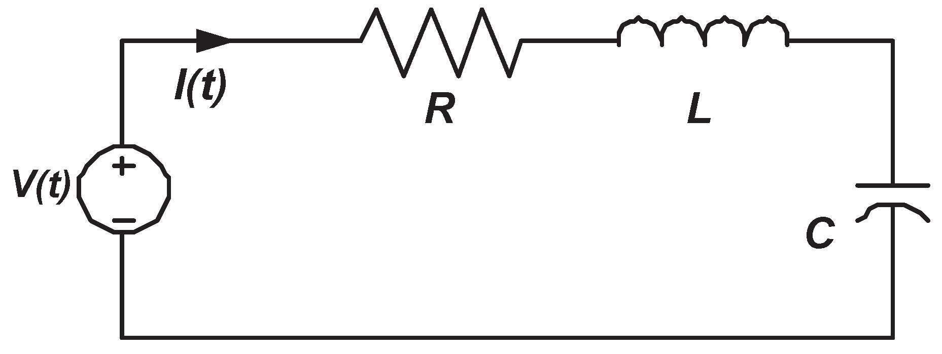
20) are recovered in the traditional sense. Applying Kirchhoff’s laws, the equation of the RLC circuit represented in
Figure 1 is given by
where
L is the inductance,
R is the resistance and the source voltage is
.
3.1. RLC Electrical Circuit via Liouville–Caputo Fractional Operator
Considering (
19) and (
20), the fractional equation corresponding to (
21) in the Liouville–Caputo sense is given by:
where
and
. Now we obtain the analytical solution of Equation (
22) considering different source terms
.
Case 1. Unit step source, , (22) is defined as followsApplying the Laplace transform (12) to (23), we have Taking the inverse Laplace transform of (
24)
, we obtain: Case 2. Exponential source, , (22) is defined as followsApplying the Laplace transform (12) to (26), the expression for the current is Taking the inverse Laplace transform to (27), the analytical solution is: Case 3. Periodic source, , (32) is defined as followsApplying the Laplace transform (12) to (29), the expression for the current is Taking the inverse Laplace transform to (30), the analytical solution is: 3.2. RLC Electrical Circuit via Caputo–Fabrizio Fractional Operator
Considering (
19) and (
20), the fractional equation corresponding to (
21) in the Caputo–Fabrizio sense is given by:
we obtain the analytical solutions of Equation (
32) considering different source terms.
Case 4. Unit step source, , (32) is defined as followsApplying the Laplace transform (12) to (33), the expression for the current is: Taking the inverse Laplace transform of (
34)
, we obtain the following solution:where Case 5. Exponential source, , (32) is defined as follows Applying the Laplace transform (12) to (37), the expression for the current is: Taking the inverse Laplace transform to (38), the analytical solution is:where M, K and L are given by (36). Case 6. Periodic source, , (32) is defined as followsApplying the Laplace transform (12) to (40), the expression for the current is: Taking the inverse Laplace transform to (41), the analytical solution is:where M, K and L are given by (36). 3.3. RLC Electrical Circuit Involving the Fractional Operator with Mittag-Leffler Kernel
Considering (
19) and (
20), the fractional equation corresponding to (
21) via the fractional operator with Mittag-Leffler kernel is given by
we obtain the analytical solutions of (
43) considering different source terms.
Case 7. Unit step source, , (43) is defined as follows:Applying the Laplace transform (16) to (44), the expression for the current is: Taking the inverse Laplace transform of (
45)
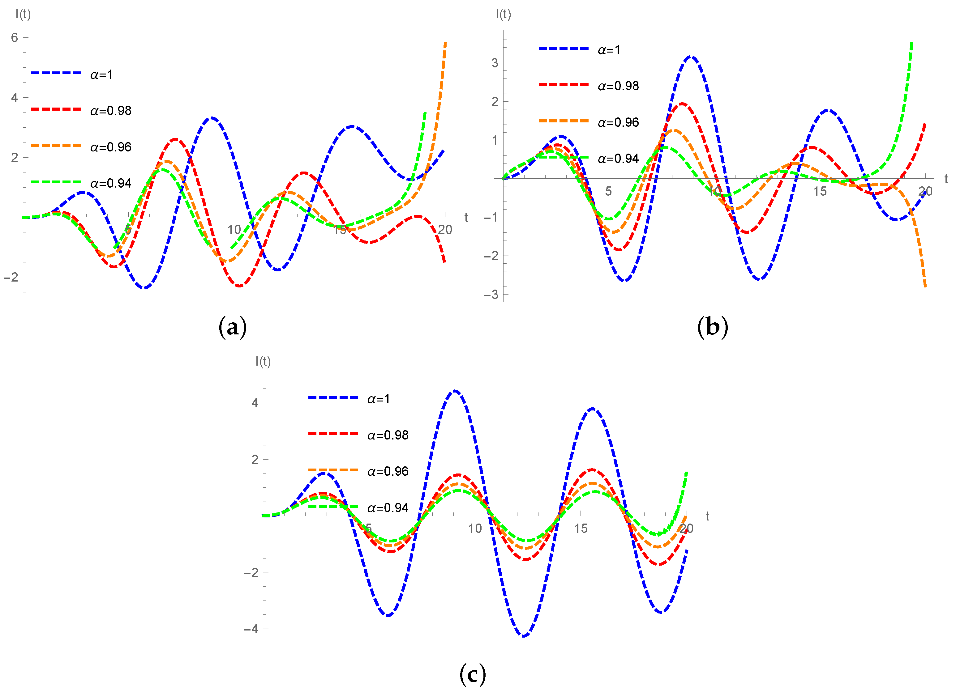
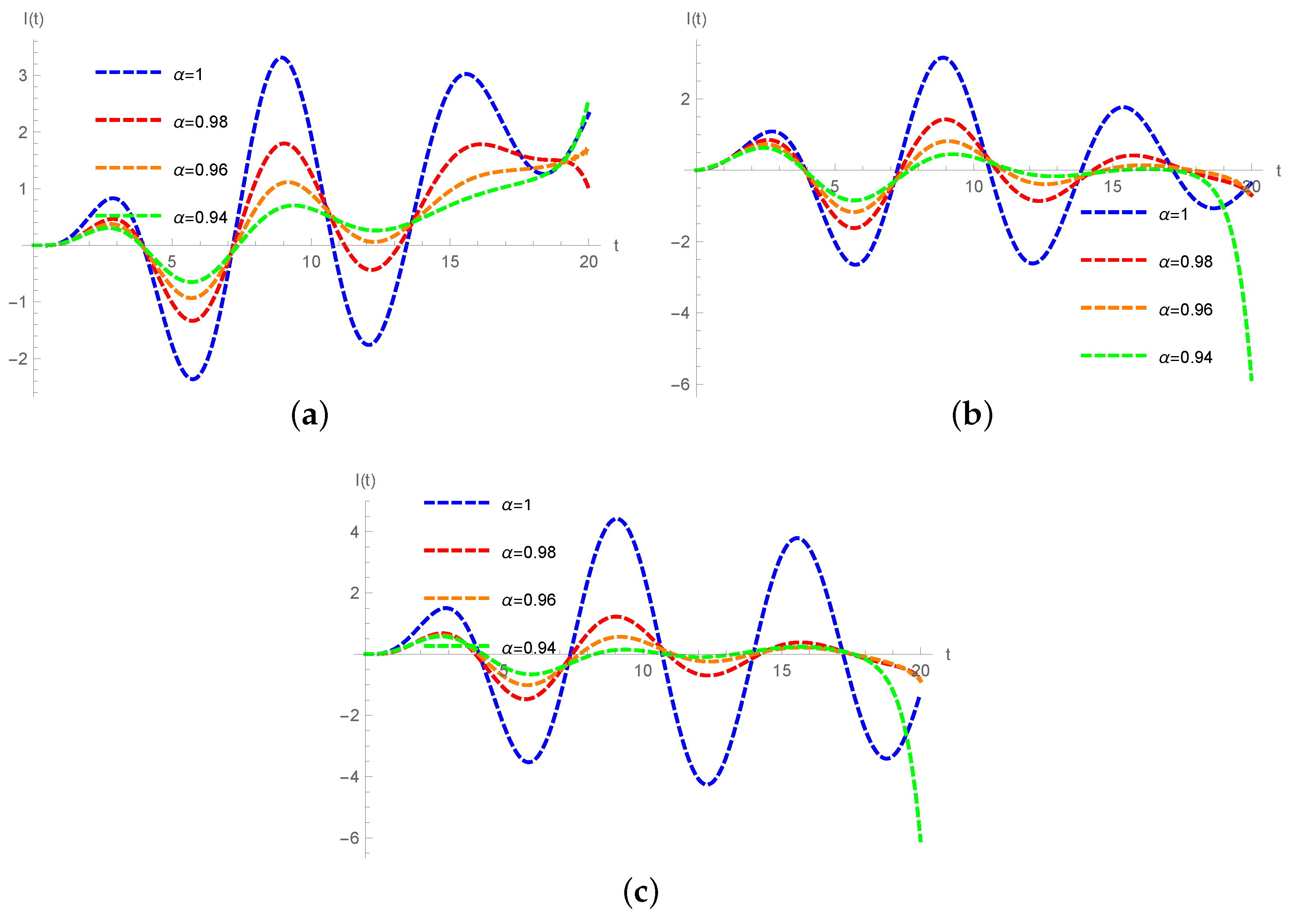
, the solution is:where Case 8. Exponential source, , (43) is defined as follows:Applying the Laplace transform (16) to (48), the expression for the current is: Taking the inverse Laplace transform to (49), the solution is:where and H are given by (47). Case 9. Periodic source, , , , , (43) is defined as follows: Applying the Laplace transform (16) to (51), the expression for the current is: Taking the inverse Laplace transform to (52), the solution is: where and H are given by (47). Example 1. Consider the electrical circuit RLC with R = 100 Ω
, H, F and V. Figure 2, Figure 3 and Figure 4 show numerical simulations for the current in the inductor, for different particular cases of α using the Liouville–Caputo, Caputo–Fabrizio and the Atangana–Baleanu–Caputo fractional operator, respectively. 4. Conclusions
In the present paper, analytical solutions of the electrical RLC circuit using the Liouville–Caputo, Caputo–Fabrizio and the Atangana–Baleanu–Caputo fractional operators were presented. The solutions obtained preserve the dimensionality of the studied system for any value of the exponent of the fractional derivative.
We can conclude that the decreasing value of α provides an attenuation of the amplitudes of the oscillations, the system increases its “damping capacity” and the current changes due to the order derivative (causing irreversible dissipative effects such as ohmic friction), the response of the system evolves from an under-damped behavior into an over-damped behavior. The fractional differentiation with respect to the time represents a non-local effect of dissipation of energy (internal friction) represented by the fractional order α. The electrical circuit RLC exhibits fractality in time to different scales and shows the existence of heterogeneities in the electrical components (resistance, capacitance and inductance). Due to the physical process involved (i.e., magnetic hysteresis), these components can present signs of nonlinear phenomena and non-locality in time, it is clear that the approximate solutions continuously depend on the time-fractional derivative α. In the classical case, where , due to the absence of damping, the amplitude is maintained and the system displays the Markovian nature.
For the Liouville–Caputo fractional operator the solutions incorporate and describe long term memory effects (attenuation or dissipation), these effects are related to an algebraic decay related to the Mittag-Leffler function. However, this fractional operator involves a kernel with singularity. The Caputo–Fabrizio fractional operator is based on the exponential function; thus, the used kernel is local and may not be able to portray more accurately some systems. Nevertheless, due to their properties, some researchers have concluded that this operator can be viewed as a filter regulator [
28]. Atangana and Baleanu presented a fractional derivative with Mittag-Leffler kernel. This derivative is the average of the given function and its Riemann–Liouville fractional integral. The Figures show that the system presents dissipative effects that correspond to the nonlinear situation of the physical process (realistic behavior that is non-local in time). Furthermore, the Figures show that the Liouville–Caputo fractional derivative is more affected by the past compared with the new fractional operator based on the Mittag-Leffler function which shows a rapid stabilization. Finally, the Caputo–Fabrizio approach is a particular case of the representation obtained using the fractional operator with thw Mittag-Leffler kernel in the Liouville–Caputo sense.
This methodology can be applied in the analysis of electromagnetic transients problems in electrical systems, machine windings, modeling of surface discharge in electrical equipment, transmission lines, power electronics, underground cables or partial discharge in insulation systems and control theory.
Acknowledgments
The authors appreciate the constructive remarks and suggestions of the anonymous referees that helped to improve the paper. We would like to thank to Mayra Martínez for the interesting discussions. José Francisco Gómez-Aguilar acknowledges the support provided by CONACYT: cátedras CONACYT para jovenes investigadores 2014. The research is supported by a grant from the “Research Center of the Center for Female Scientific and Medical Colleges”, Deanship of Scientific Research, King Saud University. The authors are also thankful to visiting professor program at King Saud University for support.
Author Contributions
The analytical results were worked out by José Francisco Gómez-Aguilar, Victor Fabian Morales-Delgado, Marco Antonio Taneco-Hernández, Dumitru Baleanu, Ricardo Fabricio Escobar-Jiménez and Maysaa Mohamed Al Qurashi; José Francisco Gómez-Aguilar, Ricardo Fabricio Escobar-Jiménez and Maysaa Mohamed Al Qurashi polished the language and were in charge of technical checking. José Francisco Gómez-Aguilar, Victor Fabian Morales-Delgado, Marco Antonio Taneco-Hernández, Dumitru Baleanu, Ricardo Fabricio Escobar-Jiménez and Maysaa Mohamed Al Qurashi wrote the paper. All authors have read and approved the final manuscript.
Conflicts of Interest
The authors declare no conflict of interest.
References
- Kaczorek, T.; Rogowski, K. Descriptor Linear Electrical Circuits and Their Properties. In Fractional Linear Systems and Electrical Circuits; Springer: Berlin/Heidelberg, Germany, 2015; pp. 81–115. [Google Scholar]
- Freeborn, T.J.; Maundy, B.; Elwakil, A.S. Fractional-order models of supercapacitors, batteries and fuel cells: A survey. Mater. Renew. Sustain. Energy 2015, 4, 1–7. [Google Scholar] [CrossRef]
- Naim, N.; Isa, D.; Arelhi, R. Modelling of ultracapacitor using a fractional-order equivalent circuit. Int. J. Renew. Energy Technol. 2015, 6, 142–163. [Google Scholar] [CrossRef]
- Gómez-Aguilar, J.F.; Escobar-Jiménez, R.F.; Olivares-Peregrino, V.H.; Benavides-Cruz, M.; Calderón-Ramón, C. Nonlocal electrical diffusion equation. Int. J. Mod. Phys. C 2015, 27, 1650007. [Google Scholar] [CrossRef]
- Gómez-Aguilar, J.F.; Baleanu, D. Solutions of the telegraph equations using a fractional calculus approach. Proc. Romanian Acad. Ser. A 2014, 15, 27–34. [Google Scholar]
- Gómez-Aguilar, J.F.; Baleanu, D. Fractional Transmission Line with Losses. Zeitschrift für Naturforschung A 2014, 69, 539–546. [Google Scholar] [CrossRef]
- Elwakil, A.S. Fractional-Order Circuits and Systems: An Emerging Interdisciplinary Research Area. IEEE Circuits Syst. Mag. 2010, 10, 40–50. [Google Scholar] [CrossRef]
- Kumar, S. Numerical Computation of Time-Fractional Fokker–Planck Equation Arising in Solid State Physics and Circuit Theory. Zeitschrift für Naturforschung A 2013, 68, 777–784. [Google Scholar]
- Tavazoei, M.S. Reduction of oscillations via fractional order pre-filtering. Signal Process. 2015, 107, 407–414. [Google Scholar] [CrossRef]
- Gómez-Aguilar, J.F. Behavior characteristics of a cap-resistor, memcapacitor, and a memristor from the response obtained of RC and RL electrical circuits described by fractional differential equations. Turk. J. Electr. Eng. Comput. Sci. 2016, 24, 1421–1433. [Google Scholar] [CrossRef]
- Bao, H.-B.; Cao, J.-D. Projective synchronization of fractional-order memristor-based neural networks. Neural Netw. 2015, 63, 1–9. [Google Scholar] [CrossRef] [PubMed]
- Bao, H.-B.; Park, J.H.; Cao, J.-D. Adaptive synchronization of fractional-order memristor-based neural networks with time delay. Nonlinear Dyn. 2015, 82, 1343–1354. [Google Scholar] [CrossRef]
- Hartley, T.T.; Veillette, R.J.; Adams, J.L.; Lorenzo, C.F. Energy storage and loss in fractional-order circuit elements. IET Circuits Devices Syst. 2015, 9, 227–235. [Google Scholar] [CrossRef]
- Gómez-Aguilar, J.F.; Razo-HernÁndez, R.; Granados-Lieberman, D. A Physical Interpretation of Fractional Calculus in Observables Terms: Analysis of the Fractional Time Constant and the Transitory Response. Revista Mexicana de Física 2014, 60, 32–38. [Google Scholar]
- Rousan, A.A.; Ayoub, N.Y.; Alzoubi, F.Y.; Khateeb, H.; Al-Qadi, M.; Quasser, M.K.; Albiss, B.A. A Fractional LC-RC Circuit. Fract. Calc. Appl. Anal. 2006, 9, 33–41. [Google Scholar]
- Ertik, H.; Çalik, A.E.; Şirin, H.; Şen, M.; Öder, B. Investigation of Electrical RC Circuit within the Framework of Fractional Calculus. Revista Mexicana de Física 2015, 61, 58–63. [Google Scholar]
- Atangana, A.; Alkahtani, B.S.T. Analysis of the Keller–Segel model with a fractional derivative without singular kernel. Entropy 2015, 17, 4439–4453. [Google Scholar] [CrossRef]
- Caputo, M.; Fabricio, M. A New Definition of Fractional Derivative without Singular Kernel. Prog. Fract. Differ. Appl. 2005, 1, 73–85. [Google Scholar]
- Lozada, J.; Nieto, J.J. Properties of a New Fractional Derivative without Singular Kernel. Prog. Fract. Differ. Appl. 2015, 1, 87–92. [Google Scholar]
- Atangana, A.; Nieto, J.J. Numerical solution for the model of RLC circuit via the fractional derivative without singular kernel. Adv. Mech. Eng. 2015, 7, 1–6. [Google Scholar] [CrossRef]
- Atangana, A.; Alkahtani, B.S.T. Extension of the resistance, inductance, capacitance electrical circuit to fractional derivative without singular kernel. Adv. Mech. Eng. 2015, 7, 1–6. [Google Scholar] [CrossRef]
- Alkahtani, B.S.T.; Atangana, A. Chaos on the Vallis Model for El Niño with Fractional Operators. Entropy 2016, 18, 100. [Google Scholar] [CrossRef]
- Gmóez-Aguilar, J.F.; Torres, L.; Ypez-Martnez, H.; Baleanu, D.; Reyes, J.M.; Sosa, I.O. Fractional Linard type model of a pipeline within the fractional derivative without singular kernel. Adv. Differ. Equ. 2016, 2016, 173. [Google Scholar] [CrossRef]
- Morales-Delgado, V.F.; Gmóez-Aguilar, J.F.; Yépez-Martínez, H.; Baleanu, D.; Escobar-Jimenez, R.F.; Olivares-Peregrino, V.H. Laplace homotopy analysis method for solving linear partial differential equations using a fractional derivative with and without kernel singular. Adv. Differ. Equ. 2016, 2016, 164. [Google Scholar] [CrossRef]
- Atangana, A.; Alqahtani, R.T. Numerical approximation of the space-time Caputo–Fabrizio fractional derivative and application to groundwater pollution equation. Adv. Differ. Equ. 2016, 2016, 156. [Google Scholar] [CrossRef]
- Batarfi, H.; Losada, J.; Nieto, J.J.; Shammakh, W. Three-Point Boundary Value Problems for Conformable Fractional Differential Equations. J. Funct. Spaces 2015, 2015, 706383. [Google Scholar] [CrossRef]
- Gmóez-Aguilar, J.F.; Yépez-Martínez, H.; Calderón-Ramón, C.; Cruz-Orduña, I.; Escobar-Jiménez, R.F.; Olivares-Peregrino, V.H. Modeling of a Mass-Spring-Damper System by Fractional Derivatives with and without a Singular Kernel. Entropy 2015, 17, 6289–6303. [Google Scholar] [CrossRef]
- Atangana, A.; Baleanu, D. New Fractional Derivatives with Nonlocal and Non-Singular Kernel: Theory and Application to Heat Transfer Model. Therm. Sci. 2016, 20, 763–769. [Google Scholar] [CrossRef]
- Alkahtani, B.S.T. Analysis on non-homogeneous heat model with new trend of derivative with fractional order. Chaos Solitons Fractals 2016, 89, 566–571. [Google Scholar] [CrossRef]
- Alkahtani, B.S.T. Chua’s circuit model with Atangana-Baleanu derivative with fractional order. Chaos Solitons Fractals 2016, 89, 547–551. [Google Scholar] [CrossRef]
- Algahtani, O.J.J. Comparing the Atangana–Baleanu and Caputo–Fabrizio derivative with fractional order: Allen Cahn model. Chaos Solitons Fractals 2016, 89, 552–559. [Google Scholar] [CrossRef]
- Coronel-Escamilla, A.; Gmóez-Aguilar, J.F.; López-López, M.G.; Alvarado-Martínez, V.M.; Guerrero-Ramírez, G.V. Triple pendulum model involving fractional derivatives with different kernels. Chaos Solitons Fractals 2016, 91, 248–261. [Google Scholar] [CrossRef]
- Atangana, A.; Koca, I. Chaos in a simple nonlinear system with Atangana–Baleanu derivatives with fractional order. Chaos Solitons Fractals 2016, 89, 447–454. [Google Scholar] [CrossRef]
- Podlubny, I. Fractional Differential Equations; Academic Press: New York, NY, USA, 1999. [Google Scholar]
© 2016 by the authors; licensee MDPI, Basel, Switzerland. This article is an open access article distributed under the terms and conditions of the Creative Commons Attribution (CC-BY) license (http://creativecommons.org/licenses/by/4.0/).


 ,
, 


