The Constant Information Radar

Abstract

The constant information radar, or CIR, is a tracking radar that modulates target revisit time by maintaining a fixed mutual information measure. For highly dynamic targets that deviate significantly from the path predicted by the tracking motion model, the CIR adjusts by illuminating the target more frequently than it would for well-modeled targets. If SNR is low, the radar delays revisit to the target until the state entropy overcomes noise uncertainty. As a result, we show that the information measure is highly dependent on target entropy and target measurement covariance. A constant information measure maintains a fixed spectral efficiency to support the RF convergence of radar and communications. The result is a radar implementing a novel target scheduling algorithm based on information instead of heuristic or ad hoc methods. The CIR mathematically ensures that spectral use is justified.

1. Introduction

The CIR was introduced in our prior work [1] in the pursuit of theoretical information bounds on the performance for joint radar-communications systems [2,3,4,5,6,7,8]. In this body of work, the estimation rate, a measure of radar tracking information as a function of time, was defined. The result is an analogous figure of merit to the communications data rate for comparison with communications users in the same spectral allocation. Hybrid radar-communications MAC bounds could then be formulated with both users measuring spectral efficiency in bits/seconds/Hz. It was noted in this work that the radar estimation rate could be time-division multiplexed with the communications user. This is achieved by fixing the mutual information value for the target tracking scenario, while modulating the target revisit time, and the CIR naturally arose from this method of joint operation.

1.1. Background

Though radar users have operated nearly unimpeded since the widespread military use of RF ranging [9], spectral congestion is quickly becoming a crisis for modern radar systems [7]. Modern communications phenomenology has adapted to dynamic spectrum needs both in terms of technology and regulatory structure due to the rapidly increasing need for bandwidth in consumer applications [10]. This has given rise to cognitive radios and massive MIMO communications systems [11], but the same has not been true of radar. In fact, cognitive radar typically implies data-driven adaptation to complex environments, dynamic clutter configurations and complicated target scenarios, not intelligent spectrum sharing [12,13]. In response to the growing problem of spectral congestion, reactive solutions have emerged that rely on the traditional approach of static isolation in either time, frequency or space [14,15,16,17], avoiding RF convergence.

Researchers have only recently begun to look at radar scheduling as an application for cognitive systems [18], focusing on RF convergence of radar with contending communications users. Some research threads have investigated cognitive techniques to estimate communications channel parameters to reduce the mutual interference between a primary communications user and a secondary radar user [19]. Others have adapted waveforms to signal-dependent interference from communications users [20]. Considering the radar as the primary user, cognitive radio systems have employed ELINT techniques to perform blind spectrum sensing of radars similar to the task completed for competing communications only users [21]. In fact, some researchers have developed cognitive radar architectures that resemble cognitive radio much more closely by employing similar spectrum sensing techniques, emitter localization and power allocation to avoid interference with cognitive users [22]. Researchers have noted, however, that intelligent metrics beyond those in traditional radar phenomenology are still needed in future cognitive radar systems [23].

Almost immediately following the introduction of information theory by Shannon [24], Woodward applied the concept of probability and information to radar processing [25,26]. Bell’s seminal work investigated information-based waveform design [27], but for a statistical scatterer and RCS estimation, not for radar tracking. Other researchers developed cognitive techniques to extend prior work in information-theoretic waveform design for RCS estimation and target detection to include a communications user sharing the same waveform [28,29]. Information-based techniques have also been researched for intelligent target scheduling in a cognitive framework [30]. However, this work considers scheduling with multiple radar users, similar to classical cognitive radios with communications-only users. Preliminary work has also compared the cognitive operation of both users independently and jointly [31]. Tracking information has been used in the context of radar waveform design, but for limited applications and 1D scenarios [32]. Some works have investigated variable radar resolution cell sizes to keep the Fisher information constant [33]; not in an effort to modulate radar spectral access, but rather to vary the computational resolution for compressive sensing applications. Similar concepts exploiting sparsity with respect to tracking have been explored [34], but not in an information-theoretic sense. Recent research explored using data-driven techniques to supplement estimated clutter distributions to adapt to changing detection statistics [35]. In addition, extensions to Bell’s work have been made to employ mutual information-based waveform design to facilitate automated target recognition [36]. However, these techniques do not account for tracking estimation information. Some research looked at modulating revisit time based on predicted state covariance error thresholding [37]. However, this does not take into account the measurement transform and, thus, the true information available through target revisit. Others have attempted to modulate dwell time on the target based on RCS to maintain a fixed SNR, as well [38].

Some researchers have defined radar information to develop joint radar-communications information bounds [39,40], but neither consider tracking information or modulate spectral access based on radar information. Others have jointly maximized the information criterion for radar and communications users to minimize mutual interference by varying radar waveform and communications OFDM parameters in response to dynamic bandwidth allocation [41].

1.2. Contributions

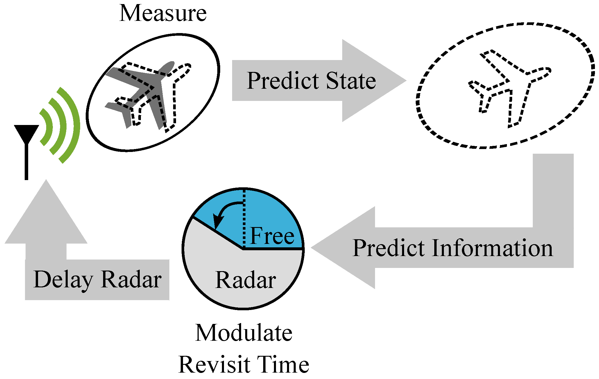
In this work, we formally develop the CIR and the corresponding scheduling concept, which is depicted at a high level in Figure 1. The radar is in track-mode and performs the typical Kalman filtering prediction steps. From the predicted state, the estimation rate is also predicted. The mutual information between the noiseless and noisy target state is estimated using the predicted SNR and the previous Kalman residual (a measure of state prediction error). The operator sets a constant information value, and the radar modulates the revisit time of the target track to attempt to keep the information measure constant. If the previous Kalman residual is large in magnitude, this indicates that the target is deviating from the predicted motion model, and the radar sets a shorter revisit time. If the predicted SNR is low, then the information content is also low, even for dynamic targets. The CIR subsequently sets a longer revisit time to allow the state uncertainty to grow large enough to overcome the measurement noise variance. This modulation of revisit time maintains a fixed radar spectral efficiency instead of suboptimally sampling the target at a regular interval. For well-modeled or low-SNR targets, this scheme allows for increased spectral access time for cognitive communications users or scheduling of additional radar targets. In our earlier work [1], we introduced the concept of maintaining constant information as a radar resource management method. Here, we more thoroughly develop the constant information radar and present more results relating to spectrum sharing. The principle contributions are as follows:

• Review the estimation rate for tracking radars
• Examine the traditional target Kalman model
• Augment tracking to include predicted estimation information
• Motivate CIR radar using predicted information
• Demonstrate the results of the CIR in a simulation compared to a traditional radar

The remainder of the article is organized as follows. Starting next with Section 2, the target tracking model is introduced as a key component to the CIR, in addition to the measurement model that supports the observation. The predicted target information is then discussed in Section 3 to augment the Kalman filter prediction step and outline the CIR scheduling algorithm for setting the target revisit time. How model mismatch and SNR modulate revisit time is analyzed in Section 4. Finally, a few tracking scenario example simulations with the CIR in action are presented in Section 5, and concluding remarks are made in Section 6.

2. Radar Tracking and Measurement Model

The radar tracking model is critical to the CIR framework. The model forms a hypothesis for the target state based on prior physical knowledge and the previously-estimated state, typically involving a position and velocity component. Based on classical physics, we can predict where the target will be after time T later. For more advanced models, this can include compensation for acceleration and higher order motion components. Here, we assume, for simplicity and illustration, a constant velocity model. We start our formulation at the source and work through the measurement model to capture the interdependencies. The most natural formulation to that end is to use a dynamical Markov model as a part of a tracking process, followed by a range, range-rate, and bearing measurement model.

2.1. Target Motion Model

For the target motion, we assume a constant velocity, linear 2D motion model with a Gaussian perturbation acceleration distribution [42]:

$${\underline{s}}_k=\left[\begin{array}{c}{x}_k\\ {\dot{x}}_k\\ y_k\\ {\dot{y}}_k\end{array}\right]=\mathbf{A}\left(T\right){\underline{s}}_{k-1}+{\underline{w}}_k=\left[\begin{array}{cccc}1& T& 0& 0\\ 0& 1& 0& 0\\ 0& 0& 1& T\\ 0& 0& 0& 1\end{array}\right]\left[\begin{array}{c}{x}_{k-1}\\ {\dot{x}}_{k-1}\\ y_{k-1}\\ {\dot{y}}_{k-1}\end{array}\right]+{\underline{w}}_k,$$

(1)

where the ${\underline{w}}_k$ is the process noise with covariance defined as:

$${\mathbf{Q}}_k\left(T\right)=\left[\begin{array}{cccc}{q}_{x,k}\frac{T^3}{3}& q_{x,k}\frac{T^2}{2}& 0& 0\\ q_{x,k}\frac{T^2}{2}& q_{x,k}T& 0& 0\\ 0& 0& q_{y,k}\frac{T^3}{3}& q_{y,k}\frac{T^2}{2}\\ 0& 0& q_{y,k}\frac{T^2}{2}& q_{y,k}T\end{array}\right],$$

(2)

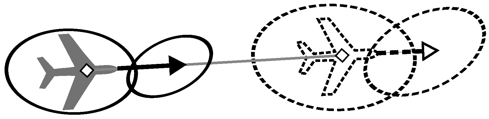
$x_k$ is the target position along the x-axis at discrete time step k; ${\dot{x}}_k$ is the target velocity projected on the x-axis; T is the revisit time of a particular target (duration between time steps k and $k-1$); ${\underline{s}}_k$ is the state vector; and $q_{x,k}$ is the process model error intensity for the x-axis (similarly for the y-axis). We assume that the x-position and velocity have an independent process noise power from the y-position and velocity. These powers are estimated to track model mismatch along each dimension. We have parameterized the linear motion model matrix $\mathbf{A}\left(T\right)$ and the process noise covariance ${\mathbf{Q}}_k\left(T\right)$ by the revisit time T, as this is our dynamic parameter. An illustration of the motion model and target prediction is shown in Figure 2.

The revisit time is a key parameter for tracking radar systems, as it specifies the amount of time between illuminations for a specific target. Between track points, the radar predicts the next target location T seconds later based on the previous target state. If T is set too large, the time between target illuminations may be too great, and the target may not be within the beamwidth of the radar beam steered to the predicted angular target location. If T is too small, ambiguous range measurements, high average power and heavy spectral use can occur. Depending on the Swerling target model [43], some tracking systems may define T to be the PRI instead of the target revisit time.

This model can easily be extended to 3D space as needed and may include more advanced motion dynamics, such as acceleration. A more advanced predictive model results in a better tracker, yielding a smaller Kalman residual, assuming the prior knowledge of the target is accurate. This theoretically reduces the true measurement deviation, an important point we discuss later.

2.2. Target Measurement Model

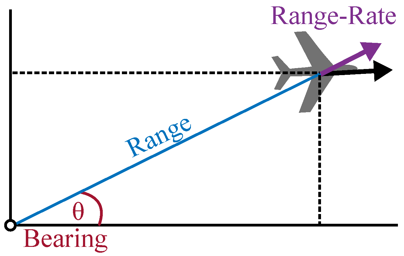
The observed parameters, after cross-ambiguity processing [44,45], are the range $r_k$ and range-rate ${\dot{r}}_k$. We assume a narrowband environment, such that only a Doppler shift is induced in the returned waveform, not the more general Doppler time scaling (though the model can easily be extended to encompass this). We also obtain a bearing measurement from our antenna array. We assume we have a phased array with half-wavelength spacing and that the platform is steerable, so the beam can be formed normal to the array at the predicted target bearing. The actual distributions for the range, range-rate and bearing are very complicated assuming an underlying Gaussian source model noise distribution [3]. We can simplify the analysis by linearizing the measurement model about the predicted state, much like the extended Kalman filter [3,46]. This results in a time-varying, but linear transform on our Gaussian state vector, resulting in another multivariate Gaussian. This source to measurement transformation is illustrated in Figure 3.

We only consider a single target scenario to compare with prior work for simplicity. We are assuming the CRLB is achievable and sufficiently high target SNR, such that only local, main lobe errors contribute to performance degradation [45]. Subsequently, our range and range-rate are corrupted by correlated Gaussian noise (correlated between the range and range-rate measurement, but independent in time). The bearing measurement is corrupted by AWGN at the CRLB, independent of the Doppler noise [11]. The results here can easily be extended to include global ambiguity using the method of interval errors [4,11,47].

Extending the tracking model to multiple targets with more complicated error models in theory only amounts to more complicated probability distributions. This is important, as our predicted mutual information depends solely on the Markov tracking distributions. Therefore, as long as distributions can be formulated for a given scenario, the mutual information can be computed, or at least bounded [48], enabling the CIR to modulate revisit time.

3. Target Tracking Information

In this section, we augment the classical Kalman filtering model to include target state information. We start by defining the estimation rate, a measure of radar tracking information as a function of time that quantifies the average bits/second required to represent information learned about a target through measurement. This quantity includes a notion of detection, as any probability distribution can be used to derive an entropy. For the linearized Kalman tracking problem here, the estimation rate is a function of the model covariance and measurement covariance. Both of these are included in the standard Kalman formulation, and so predicted information is easily incorporated into the framework.

3.1. Radar Estimation Rate

To measure the information of the target, we leverage previous works defining estimation rate [2,3,4,5,6,7,8]. The estimation rate is defined as the mutual information between the noiseless and noisy target tracking state per unit time. The noise can encompass any perturbative distribution, such as clutter distributions. The target state can include position and velocity components as described in the previous section. The mutual information can be calculated over the PRI or the target revisit period, as we do here. The result is an information flow for the radar channel. It is generally defined as [2]:

$$R_{est}=\frac{I\left(\mathbf{X};\mathbf{Y}\right)}{T},$$

(3)

where $I\left(\mathbf{X};\mathbf{Y}\right)$ is the mutual information between the noiseless state measurement $\mathbf{X}$ and the corrupted state measurement $\mathbf{Y}$ over the revisit period T.

For our scenario, we assume a Gaussian state distribution and linearize the measurement using the extended Kalman filter corrupted by an independent and additive Gaussian distribution. Therefore, the estimation rate of our target is given by [1]:

$$R_{\mathrm{est}}\le \frac{1}{2T}{log}_2\left[\frac{|\mathbf{C}{\mathbf{P}}_{k|k-1}{\mathbf{C}}^{†}+\Sigma |}{|\Sigma |}\right],$$

(4)

where $|·|$ is the determinant function, ${\mathbf{P}}_{k|k-1}$ is the predicted model covariance, $\mathbf{C}$ is the linearized measurement transform and Σ is the inverse FIM [49], scaled by the integrated SNR given by [3]:

$$\Sigma =\frac{{\mathbf{J}}^{-1}}{\mathrm{ISNR}},$$

(5)

where $\mathbf{J}$ is the FIM, and the integrated SNR for our scenario is given by [3]:

$$\mathrm{ISNR}=\frac{N_p{T}_{p}B{P}_t{G}^2{c}^2\sigma }{f_c^2{\left(4\pi \right)}^3{r}^4{k}_N{T}_{\mathrm{temp}}B},$$

(6)

where $N_p$ is the number of pulses over the CPI, $T_p$ is the pulse duration, B is the pulse bandwidth, $P_t$ is the radar transmit power, G is gain of the radar antenna, c is the speed of light, σ is the RCS, $f_c$ is the carrier frequency of the radar waveform, r is the range to the target, $k_N$ is the Boltzmann constant and $T_{\mathrm{temp}}$ is absolute temperature of the receiver.

The form of Equation (4) is well known and arises due to the Kalman filtering formulation. The source uncertainty is our desired information and is modeled as a multivariate Gaussian with covariance ${\mathbf{P}}_{k|k-1}$. This covariance is obtained by taking the last target distribution at time step $k-1$ and advancing the prediction in time using the linear motion model $\mathbf{A}$:

$${\mathbf{P}}_{k|k-1}=\mathbf{A}\left(T\right){\mathbf{P}}_{k-1}\mathbf{A}{\left(T\right)}^{†}+{\mathbf{Q}}_k\left(T\right).$$

(7)

The covariance of the measured distribution, after linearizing about the predicted state, is given by ${\mathbf{C}}^{†}{\mathbf{P}}_{k|k-1}\mathbf{C}$, where $\mathbf{C}$ is the Jacobian of the measurement matrix linearized about the predicted state. The linear transform of the multivariate Gaussian results in another multivariate Gaussian. Finally, this source distribution is corrupted at the receiver by Gaussian noise with covariance Σ independent from the source uncertainty. In general, the range and range-rate noise are correlated as they are coupled at the matched filter, while the bearing measurement noise is independent. The mutual information between the corrupted measurement and the noiseless measurement is then presented in the form given by Equation (4) [50].

For our case of 2D tracking using range, bearing and Doppler measurements, the scaled inverse FIM is given by (assuming a Gaussian time window and a flat spectrum) [43,45]:

$$\Sigma =\frac{1}{\mathrm{ISNR}}\left[\begin{array}{ccc}\frac{T_p{c}^2}{4}& -\frac{T_{p}B{c}^2}{2f_c}& 0\\ -\frac{T_{p}B{c}^2}{2f_c}& {\left(\frac{c}{T_{p}4\pi f_c}\right)}^2+{\left(\frac{Bc}{f_c}\right)}^2& 0\\ 0& 0& \frac{6}{{\pi }^2{cos}^2(\Delta \theta )N_A(N_A^2-1)}\end{array}\right],$$

(8)

where $\Delta \theta$ is the difference between the predicted bearing and the true target bearing and $N_A$ is the number of antenna array elements. Finally, the linearization matrix is given by computing the Jacobian of the measurement matrix [3,46]:

$$\mathbf{C}=\left[\begin{array}{cccc}\frac{2}{c}\frac{\partial R}{\partial x}& \frac{2}{c}\frac{\partial R}{\partial \dot{x}}& \frac{2}{c}\frac{\partial R}{\partial y}& \frac{2}{c}\frac{\partial R}{\partial \dot{y}}\\ \frac{2{\omega }_c}{c}\frac{\partial \dot{R}}{\partial x}& \frac{2{\omega }_c}{c}\frac{\partial \dot{R}}{\partial \dot{x}}& \frac{2{\omega }_c}{c}\frac{\partial \dot{R}}{\partial y}& \frac{2{\omega }_c}{c}\frac{\partial \dot{R}}{\partial \dot{y}}\\ \frac{\partial \mathrm{\Theta }}{\partial x}& \frac{\partial \mathrm{\Theta }}{\partial \dot{x}}& \frac{\partial \mathrm{\Theta }}{\partial y}& \frac{\partial \mathrm{\Theta }}{\partial \dot{y}}\end{array}\right],$$

(9)

where R, $\dot{R}$ and Θ are the measurement functions for the range, range-rate and bearing, respectively, and the partial derivatives are all to be evaluated at the predicted state. For the range, we get the following:

$$\begin{array}{cc}\hfill \frac{\partial R}{\partial x}& =\frac{\partial }{\partial x}\left[\sqrt{x^2+y^2}\right]{|}_{\{x,y\}={\{x,y\}}_{k|k-1}}=\frac{x_{k|k-1}}{\sqrt{x_{k|k-1}^2+y_{k|k-1}^2}}\hfill \\ \hfill \frac{\partial R}{\partial \dot{x}}& =\frac{\partial }{\partial \dot{x}}\left[\sqrt{x^2+y^2}\right]{|}_{\{x,y\}={\{x,y\}}_{k|k-1}}=0\hfill \\ \hfill \frac{\partial R}{\partial y}& =\frac{\partial }{\partial y}\left[\sqrt{x^2+y^2}\right]{|}_{\{x,y\}={\{x,y\}}_{k|k-1}}=\frac{y_{k|k-1}}{\sqrt{x_{k|k-1}^2+y_{k|k-1}^2}}\hfill \\ \hfill \frac{\partial R}{\partial \dot{y}}& =\frac{\partial }{\partial \dot{y}}\left[\sqrt{x^2+y^2}\right]{|}_{\{x,y\}={\{x,y\}}_{k|k-1}}=0\hfill \end{array}$$

(10)

For the range-rate, we get the following:

$$\begin{array}{cc}\hfill \frac{\partial \dot{R}}{\partial x}& =\frac{\partial }{\partial x}\left[\frac{x\dot{x}+y\dot{y}}{\sqrt{x^2+y^2}}\right]{|}_{\underline{s}={\underline{s}}_{k|k-1}}=\frac{{\dot{x}}_{k|k-1}}{\sqrt{x_{k|k-1}^2+y_{k|k-1}^2}}-\frac{x_{k|k-1}^2{\dot{x}}_{k|k-1}+y_{k|k-1}{\dot{y}}_{k|k-1}{x}_{k|k-1}}{{\left(\sqrt{x_{k|k-1}^2+y_{k|k-1}^2}\right)}^3}\hfill \\ \hfill \frac{\partial \dot{R}}{\partial \dot{x}}& =\frac{\partial }{\partial \dot{x}}\left[\frac{x\dot{x}+y\dot{y}}{\sqrt{x^2+y^2}}\right]{|}_{\underline{s}={\underline{s}}_{k|k-1}}=\frac{x_{k|k-1}}{\sqrt{x_{k|k-1}^2+y_{k|k-1}^2}}\hfill \\ \hfill \frac{\partial \dot{R}}{\partial y}& =\frac{\partial }{\partial y}\left[\frac{x\dot{x}+y\dot{y}}{\sqrt{x^2+y^2}}\right]{|}_{\underline{s}={\underline{s}}_{k|k-1}}=\frac{{\dot{y}}_{k|k-1}}{\sqrt{x_{k|k-1}^2+y_{k|k-1}^2}}-\frac{x_{k|k-1}{\dot{x}}_{k|k-1}{y}_{k|k-1}+y_{k|k-1}^2{\dot{y}}_{k|k-1}}{{\left(\sqrt{x_{k|k-1}^2+y_{k|k-1}^2}\right)}^3}\hfill \\ \hfill \frac{\partial \dot{R}}{\partial \dot{y}}& =\frac{\partial }{\partial \dot{y}}\left[\frac{x\dot{x}+y\dot{y}}{\sqrt{x^2+y^2}}\right]{|}_{\underline{s}={\underline{s}}_{k|k-1}}=\frac{y_{k|k-1}}{\sqrt{x_{k|k-1}^2+y_{k|k-1}^2}}\hfill \end{array}$$

(11)

Finally, for the bearing, we get the following:

$$\begin{array}{cc}\hfill \frac{\partial \mathrm{\Theta }}{\partial x}& =\frac{\partial }{\partial x}\left[\mathrm{atan}2\left(y,x\right)\right]{|}_{x,y=x_{k|k-1},y_{k|k-1}}=\frac{-y_{k|k-1}}{x_{k|k-1}^2+y_{k|k-1}^2}\hfill \\ \hfill \frac{\partial \mathrm{\Theta }}{\partial \dot{x}}& =\frac{\partial }{\partial \dot{x}}\left[\mathrm{atan}2\left(y,x\right)\right]{|}_{x,y=x_{k|k-1},y_{k|k-1}}=0\hfill \\ \hfill \frac{\partial \mathrm{\Theta }}{\partial y}& =\frac{\partial }{\partial y}\left[\mathrm{atan}2\left(y,x\right)\right]{|}_{x,y=x_{k|k-1},y_{k|k-1}}=\frac{x_{k|k-1}}{x_{k|k-1}^2+y_{k|k-1}^2}\hfill \\ \hfill \frac{\partial \mathrm{\Theta }}{\partial \dot{y}}& =\frac{\partial }{\partial \dot{y}}\left[\mathrm{atan}2\left(y,x\right)\right]{|}_{x,y=x_{k|k-1},y_{k|k-1}}=0\hfill \end{array}$$

(12)

Note that because this linearization occurs about the predicted state, $\mathbf{C}$ implicitly also depends on the target revisit time T, as this modifies the predicted state.

If the information changes for each target revisit, then $R_{\mathrm{est}}$ fluctuates. Instead, we can focus on the mutual information and attempt to keep it constant by modulating the revisit time T:

$$I_{const}^{\prime }=\frac{1}{2}{log}_2\left[\frac{|\mathbf{C}{\mathbf{P}}_{k|k-1}{\mathbf{C}}^{†}+\Sigma |}{|\Sigma |}\right].$$

(13)

This way, each time we visit the target, we stand to gain the same amount of information. It is important to note that ${\mathbf{P}}_{k|k-1}$, $\mathbf{C}$ and Σ all depend on the revisit time for which we are solving: $\mathbf{C}$ as previously discussed, ${\mathbf{P}}_{k|k-1}$ through the motion model $\mathbf{A}\left(T\right)$ and process noise covariance ${\mathbf{Q}}_k\left(T\right)$ (both of which contain T as a term) and Σ through the predicted SNR.

In addition to the target process noise, another source of information must be accounted for: probability of detection. This can be done by assuming we have two channels, the detection channel and the empty channel. The detection channel is used by the target to communicate with the radar (unwillingly) with probability $P_D$, while the empty channel is used with probability $1-P_D$. The detection channel communicates at a rate $R_{\mathrm{est}}$ defined in Equation (4), while the empty channel has zero rate. It can be shown [50] that the general capacity is defined as:

$$C=H\left(P_D\right)+P_D{C}_{\det }+\left(1-P_D\right)C_{\varnothing },$$

(14)

where $H\left(P_D\right)$ is the entropy of a Bernoulli distribution parameterized by $P_D$ [50], $C_{\det }$ is the capacity of the detection channel and $C_{\varnothing }$ is the capacity of the empty channel. The proof is as follows. If we let D be an indicator random variable where $D=1$ if we detect the target and $D=0$ if we do not, then the mutual information is derived using basic information theory identities [50]:

$$\begin{array}{ccc}I\left(\mathbf{X};\mathbf{Y}\right)\hfill & =& h\left(\mathbf{Y}\right)-h\left(\mathbf{Y}|\mathbf{X}\right)\hfill \\ & =& h\left(\mathbf{Y},D\right)-H\left(D|\mathbf{Y}\right)-h\left(\mathbf{Y}|\mathbf{X},D\right)-I\left(\mathbf{Y};D|\mathbf{X}\right)\hfill \\ & =& h\left(\mathbf{Y},D\right)-h\left(\mathbf{Y}|\mathbf{X},D\right)\hfill \\ & =& H\left(D\right)+h\left(\mathbf{Y}|D\right)-h\left(\mathbf{Y}|\mathbf{X},D\right)\hfill \\ & =& H\left(D\right)+I\left(\mathbf{X};\mathbf{Y}|D\right)\hfill \\ & =& H\left(P_D\right)+P_{D}I\left(\mathbf{X};\mathbf{Y}|D=1\right)+\left(1-P_D\right)I\left(\mathbf{X};\mathbf{Y}|D=0\right)\hfill \\ & =& H\left(P_D\right)+P_D{C}_{\det }+\left(1-P_D\right)C_{\varnothing }\hfill \end{array}$$

(15)

We can now define the more general estimation information as follows:

$$I_{\mathrm{const}}=P_D{I}_{\mathrm{const}}^{\prime }-P_D{log}_2\left[P_D\right]-\left(1-P_D\right){log}_2\left[1-P_D\right].$$

(16)

Making a hard decision about target detection is sub-optimal, and so, the form given by Equation (16) can be thought of as a worst case bounding the potential performance. For example, TBD methods could be used with an augmented state space to include detection or with a discrete Markov chain layered on top of the normal tracking filter [51]. The extension of this work to include these distributions requires only solving for the mutual information of the more complicated densities.

The goal is now to select the target revisit time T such that the predicted information is given by the value calculated in Equation (16).

3.2. Target Predicted Information

We now parameterize the predicted information and solve for the estimated target revisit time to maintain our constant information, $I_{\mathrm{const}}$. This amounts to solving Equation (16) for T. Solving for this in closed form is very difficult and may not be possible. The term T appears in $\mathbf{A}\left(T\right)$ and $\mathbf{Q}\left(T\right)$, both of which drive ${\mathbf{P}}_{k|k-1}$ in Equation (13). It also appears indirectly in $\mathbf{C}$, since the linearization is about the predicted state, which depends on T, as well. Finally, the predicted range depends on T, which drives a predicted SNR given in Equation (6) and, ultimately, a prediction for Σ. Therefore, all three matrices in Equation (13) depend on T in a highly nonlinear way. Further, the dual channel form including the probability of detection in Equation (16) includes the term $P_D$, which also depends on T through the predicted SNR.

To simplify solving for T, we evaluate the information for each entry in a table of M revisit times $\mathbf{T}$ to determine the best new revisit time among the table values, $T_{\mathrm{next}}$. The steps for predicting the information and picking the nearest revisit time in the table are summarized in Algorithm 1, where $r_{k|k-1}$ is the predicted range (obtained from the predicted state ${\underline{s}}_{k|k-1}$, which contains the predicted position $\{x_{k|k-1},y_{k|k-1}\}$), ${\mathrm{ISNR}}_{k|k-1}$ is the predicted integrated SNR, $r_0$ is the reference range where the integrated SNR is unity on a linear scale, ${\Sigma }_{k|k-1}$ is the predicted scaled inverse FIM, ${\mathbf{R}}_{zz,k|k-1}$ is the predicted measurement covariance and $P_{D,k|k-1}$ is the predicted probability of detection for a fixed probability of false alarm, $P_{\mathrm{FA}}$. Note that these are the standard Kalman formulae tailored to our radar tracking problem and augmented to include the predicted information.

First, the state is predicted using the linear motion model applied to the previous state estimate. After advancing the mean, the state covariance is also modified by this transform and added to the model covariance. We can predict the range measurement from the predicted state, which directly relates to predicting the SNR and, thus, the scaled inverse FIM. The state prediction covariance is advanced through the linearized measurement model and added to the scaled inverse FIM. We have parameterized the Jacobian matrix $\mathbf{C}$ by the predicted state to emphasize the dependence of the linearization on the predicted state, which varies for each choice of $T_i\in \mathbf{T}$. Note that all of these statistics are multivariate Gaussians with linear modifiers, so Gaussianity is maintained. The probability of false alarm, a configurable system parameter, is then used to predict the probability of detection. Finally, all of the predicted quantities from the normal Kalman filtering steps can be plugged into Equation (16) to predict the mutual information for this particular value of $T_i\in \mathbf{T}$. We perform the prediction step M times to determine the revisit time $T_{\mathrm{next}}$ in the table $\mathbf{T}$ that yields predicted mutual information that is closest to $I_{\mathrm{const}}$. We do not motivate or derive the standard Kalman formulae, as it is readily accessible in the literature and extensively covered in prior work [46].

The new predicted information step of the Kalman formulation used by the CIR falls in line naturally after the normal predicted quantities, as it depends on them. Any method of model-based filtering involving distribution propagation (for example, particle filtering for highly nonlinear applications [46]) can add the information prediction step to the corresponding algorithm and subsequently apply the CIR scheduling algorithm. The tracking estimation can also be augmented with transient features like automatic target recognition, where the information from the classification distribution would drive an initially higher sampling rate to reduce classification uncertainty or wait to interrogate the target more rapidly when the predicted state indicated recognition would be more favorable.

Algorithm 1 Revisit Time Modulation (Solving for T)

$\mathbf{T}=\{T_1,T_2,...,T_M\}$ (Revisit Time Table) for $i=1:M$ do     Pick $T_i\in \mathbf{T}$ (Hypothesis Revisit Time)     ${\underline{s}}_{k|k-1}=\mathbf{A}\left(T_i\right){\underline{s}}_{k-1}$ (State Prediction)     ${\mathbf{P}}_{k|k-1}=\mathbf{A}\left(T_i\right){\mathbf{P}}_{k-1}\mathbf{A}{\left(T_i\right)}^{†}+{\mathbf{Q}}_k\left(T_i\right)$ (Source Covariance Prediction)     $r_{k|k-1}=\sqrt{x_{k|k-1}^2+y_{k|k-1}^2}$ (Range Prediction)     ${\mathrm{ISNR}}_{k|k-1}=r_0^4/r_{k|k-1}^4$ (SNR Prediction)     ${\Sigma }_{k|k-1}={\mathbf{J}}^{-1}/{\mathrm{ISNR}}_{k|k-1}$ (Scaled Inverse Fisher Information Prediction)     ${\mathbf{R}}_{zz,k|k-1}=\mathbf{C}({\underline{s}}_{k|k-1}){\mathbf{P}}_{k|k-1}\mathbf{C}{({\underline{s}}_{k|k-1})}^{†}+{\Sigma }_{k|k-1}$ (Measurement Covariance Prediction)     $P_{D,k|k-1}=P_{\mathrm{FA}}^{1/(1+{\mathrm{ISNR}}_{k|k-1})}$ (Probability of Detection Prediction)     $I_{T_i,k|k-1}=P_{D,k|k-1}\frac{1}{2}{log}_2\left[\frac{\left|{\mathbf{R}}_{zz,k|k-1}\right|}{\left|{\Sigma }_{k|k-1}\right|P_{D,k|k-1}^2}\right]-\left(1-P_{D,k|k-1}\right){log}_2\left[1-P_{D,k|k-1}\right]$                     (Predicted Information) end for $T_{\mathrm{next}}=\arg {min}_{T_i\in \mathbf{T}}|I_{T_i,k|k-1}-I_{\mathrm{const}}|$ (Calculated Revisit Time)

The distributions used in this work are linear and Gaussian, and so, closed forms for the predicted information exist and are mathematically tractable. More general tracking solutions can have complex distributions where the mutual information can be difficult to compute or estimate. In these cases, the CIR scheduling algorithm may still be used by applying reasonably tight bounds that can be formulated by modeling the filtering distributions as Gaussian mixture models GMMs [48] if the perturbative distributions are independent and additive.

In addition to the normal Kalman recursion, the process noise power is also recursively computed after each track point. To start, the process noise is estimated by subtracting the predicted state from the current state estimate [52]:

$${\widehat{\underline{w}}}_k={\underline{s}}_k-{\underline{s}}_{k|k-1}.$$

(17)

Since both are unbiased statistics of the true state, the result is a zero-mean Gaussian with covariance given by the sum of the covariances of the prediction and the estimate [46]. This is effectively the Kalman weighted residual [46] or innovation. We then compute the likelihood over a 2D table of hypothesis noise intensities for $q_x$ and $q_y$:

$${\underline{q}}_k={\arg min}_{\underline{q}=\left[q_x{q}_y\right]}ln\left[|\Omega \left(\underline{q}\right)|\right]+{\widehat{\underline{w}}}_k^{†}\Omega {\left(\underline{q}\right)}^{-1}{\widehat{\underline{w}}}_k,$$

(18)

where:

$$\Omega \left(\underline{q}\right)=2\mathbf{P}\left(\underline{q}\right)-\mathbf{P}\left(\underline{q}\right){\mathbf{C}}^{†}{\mathbf{R}}_{zz,k|k-1}^{-1}\mathbf{C}\mathbf{P}\left(\underline{q}\right),$$

(19)

and

$$\mathbf{P}\left(\underline{q}\right)=\mathbf{A}\left(T\right){\mathbf{P}}_{k-1}\mathbf{A}{\left(T\right)}^{†}+\left[\begin{array}{cccc}{q}_x\frac{T^3}{3}& q_x\frac{T^2}{2}& 0& 0\\ q_x\frac{T^2}{2}& q_{x}T& 0& 0\\ 0& 0& q_y\frac{T^3}{3}& q_y\frac{T^2}{2}\\ 0& 0& q_y\frac{T^2}{2}& q_{y}T\end{array}\right],$$

(20)

and ${\mathbf{R}}_{zz,k|k-1}$ denotes the measurement covariance prediction as defined in Algorithm 1. The joint value that minimizes Equation (18) is chosen as an estimate for the noise intensities at that time step and used for the next time step prediction. These values are thus used in Algorithm 1 to select the next target revisit time, as they modify the predicted information.

Note that the authors expect the novel predicted information step to subsume the convergence properties of the standard Kalman filter state variables, but this extension is not explicitly covered here. This is due in part to the fact that the CIR is designed to modulate T to force the track to remain sufficiently dynamical, and therefore, convergence may not be possible for the time-varying statistics.

4. Revisit Time Modulation

Here, we discuss our motivation for modulating the target revisit time. The revisit period is modulated to maintain a constant measure of information at each radar illumination of a given target. If we predict the mutual information to be larger than the previous measurement information, then there is more uncertainty predicted and, therefore, more information to be gained from knowledge of the radar return. If we predict the mutual information will decrease from the previous measurement, then less information is predicted to be measured if we maintain a constant revisit time.

4.1. Model Mismatch

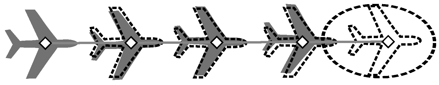
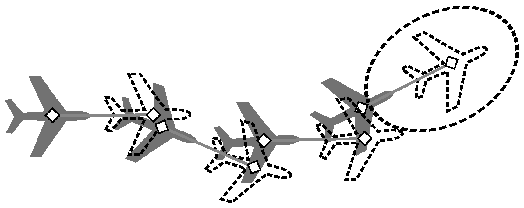
We start by looking at modulation with respect to model mismatch. As discussed in the previous sections, the radar targets have a physical motion model. When targets adhere to this model, then the prediction step is more accurate, and the true measurement offset from this prediction can be small. This is illustrated in Figure 4. The dashed outlines represent the target state prediction, while the gray planes are the actual measurements. In this work, we assume a constant velocity model, and since the plane is not accelerating appreciably, the prediction is quite accurate. As a result, the information gained through measurement may be small for this fixed revisit time.

In Figure 5, we illustrate a highly dynamic target. Instead of maintaining a constant velocity, as in our model hypothesis, the plane is maneuvering in a serpentine fashion. As a result, the difference between the prediction and measurement is larger at each track point. This increased model error uncertainty is represented in the final point shown by a larger prediction covariance contour. In this scenario, for a fixed target revisit time, more information is gained through measurement. It should be clear that the true information is in the measurement residuals, lending credence to the name “innovations.” A larger residual results in more information. A more advanced and accurate model generates a better estimator, but measurement is required less often to learn the same amount of information.

To quantify model mismatch, the model noise powers $q_{x,k}$ and $q_{y,k}$ used in Equation (2) are recursively computed as given in Equation (18). As the Kalman fusion process is completed, significant model mismatch produces a higher process noise estimate. As a result, the process noise that predicts the covariance, and thus information, for the next time step is increased. Since the target is exhibiting larger variation from the model, more information stands to be gained through measurement, and the revisit time should be decreased to maintain constant information.

Note that the model covariance is modified by the measurement transform as shown in Equation (4). Therefore, uncertainty in the state distribution may be removed or obfuscated after the measurement transforms the state. For example, only the radial projection of the target velocity vector is measured when exploiting the Doppler shift of the returned waveform. Uncertainty of the target velocity orthogonal to the radius vector of the target is not captured in the final mutual information. Therefore, uncertainty in the measurement domain with respect to the noisy measurement is the true source of information that can be gained.

4.2. Signal-to-Noise Ratio

Examining Equation (4), the other key factor affecting the modulation of the revisit period of a particular target is the SNR. Since the example shown here is a special case, this can be generalized to include the signal-to-interference ratio or the signal-to-clutter ratio. Any degrading distribution captured in the mutual information relationship can be used in calculating the estimation rate. Here, we are assuming that the thermal noise in our system is fairly consistent, so only the signal affects the SNR. If the signal level is degraded (for example, due to increased range), then the estimation rate decreases.

The estimation rate of the target may be interpreted as the minimum number of bits/second needed to encode or compress the target information. If we attempt to encode the noisy target range and range-rate from consecutive draws, noise could dominate the target dynamics. This reduces the number of required bits needed to encode the residual, since additional bits would only serve to encode unwanted noise. Subsequently, the revisit time is increased to compensate. This relationship to SNR can be thought of as an estimation analogy to joint typicality encountered in the channel capacity problem [50].

The probability of detection also affects the revisit time. For a fixed false alarm rate radar, the probability of detection is dependent only on SNR. The closer $P_D$ is to 0.5, the more information is contained in the Bernoulli distribution. However, a far more powerful relationship is the multiplication of the radar estimation rate by $P_D$ shown in Equation (16). Therefore, the probability of detection affects the estimation rate very similarly to SNR.

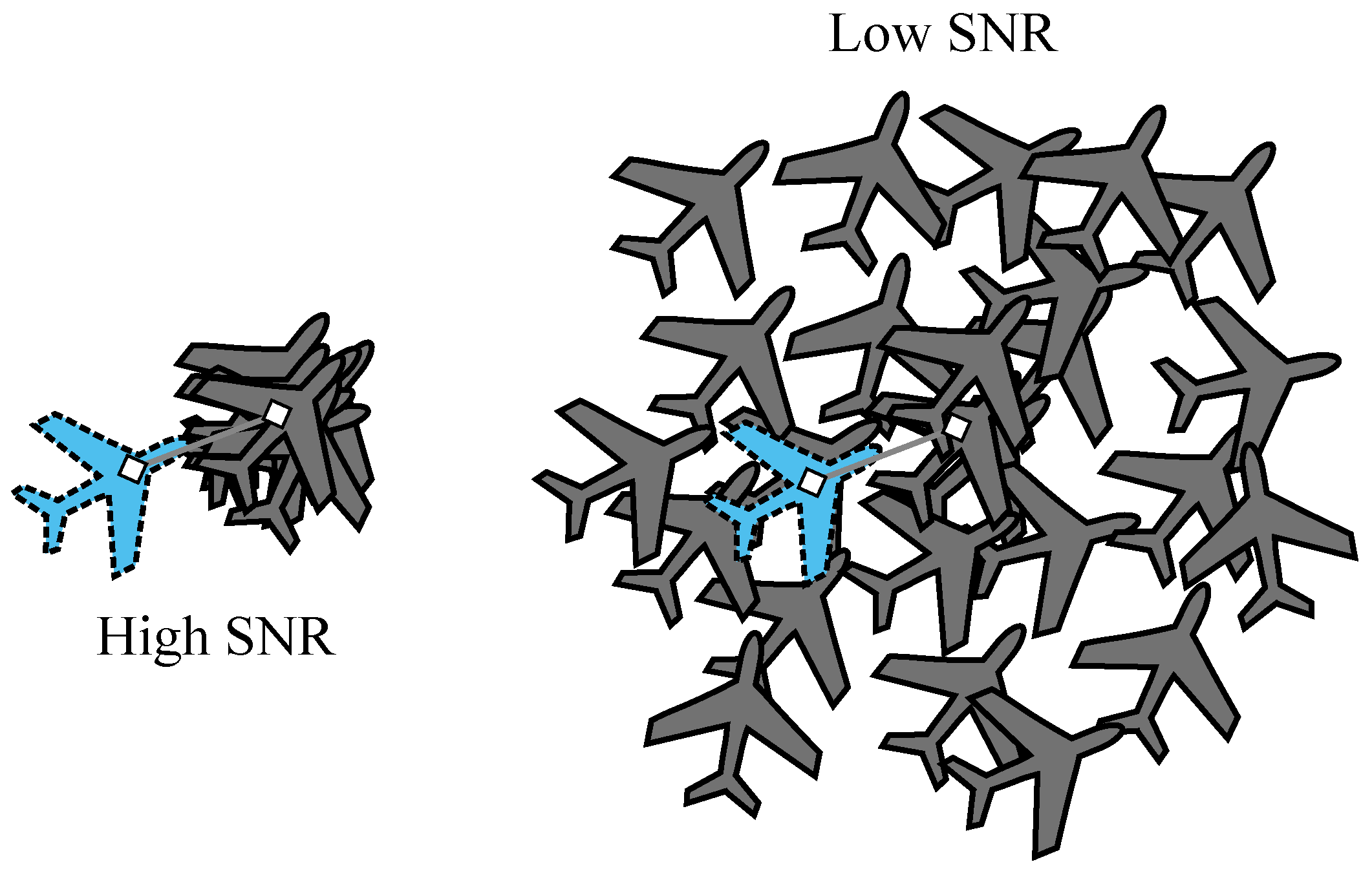
These concepts are illustrated in Figure 6 and Figure 7. The first figure shows an example of high SNR compared to low SNR. The prediction is shown in blue with the dashed outline, while the gray planes with the solid outline represent a sampling of measurements. This assumes we can essentially freeze the state of the track and measure the target multiple times. Each measurement is perturbed slightly around the true mean due to noise, clutter or interference. In the high SNR case, we can easily see the mean of the measurements offset from the prediction, and the residual contains meaningful information. For the low SNR portion of Figure 6, we see that the residual from the prediction in blue to the mean of the samples is insignificant compared to the spread of the samples. In this case, the information is low because the noise entropy is dominating the source entropy.

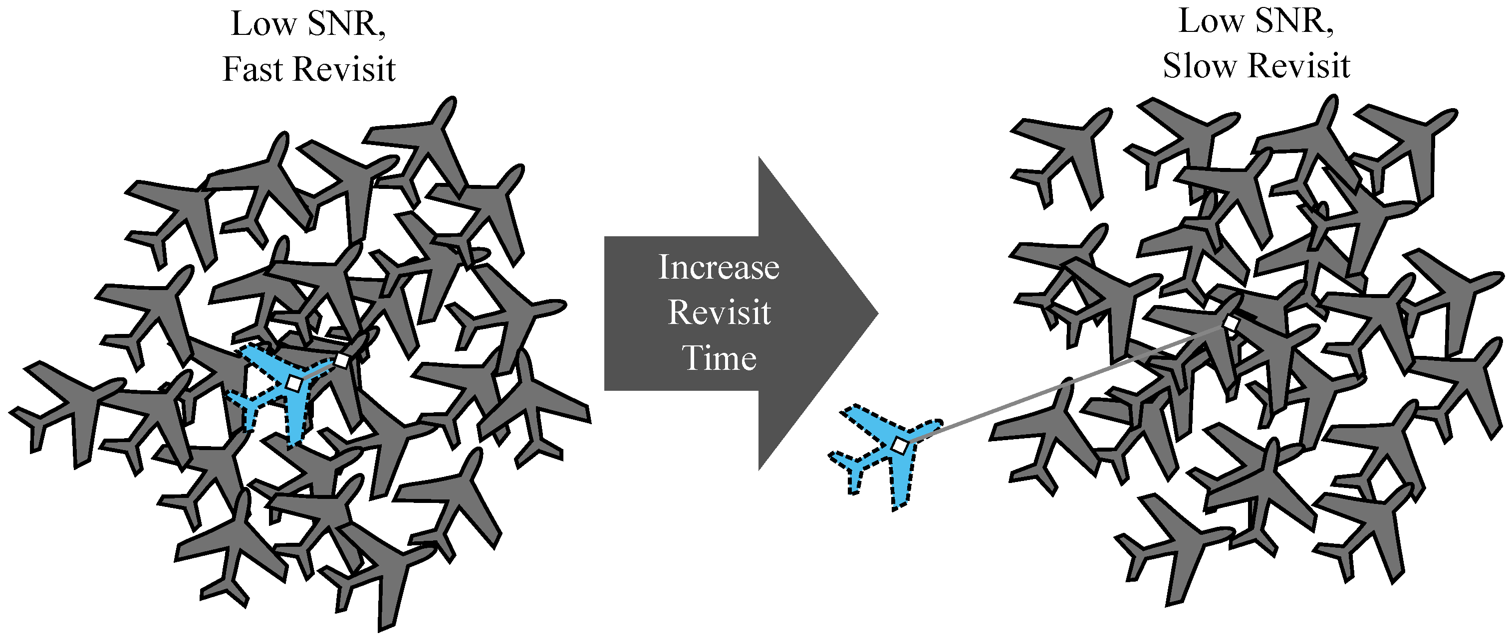
In Figure 7, we illustrate an example of how to mitigate the low SNR scenario by modulating the revisit time. When the residual is insignificant relative to measurement variance, we can delay revisiting the target for a while. At this point, our uncertainty grows, and we are less confident in our prediction since we have not measured the target in a long time to correct the target track. Measuring at this later time means we are more likely to have a measurement mean deviating more significantly from our prediction relative to the measurement spread.

5. Examples

We tested the newly-derived CIR against multiple track scenarios. The main parameters used are given in

Table 1. Parameters for example simulations.

Parameter	Value	Parameter	Value
Bandwidth (B)	5 MHz	Center Frequency ($f_c$)	3 GHz
Absolute Temperature ($T_{\mathrm{temp}}$)	1000 K	Pulse Duration ($T_p$)	5 µs
Probability of False Alarm (P${}_{\mathrm{FA}}$)	${10}^{-6}$	Radar Antenna Gain (G)	30 dBi
Radar Transmit Power ($P_t$)	100 kW	Target Cross-Section (σ)	10 m${}^2$
Chirp Rate	$B/T_p$	Window Variance	$T_p$
Wave Speed (c)	$3\times {10}^8$ m/s	Number of Pulses ($N_P$)	10
$I_{\mathrm{const}}$	Varied	Number of Array Elements ($N_A$)	10

. The CRLB was formulated assuming a linear FM waveform with a Gaussian window [45], which depends on the RMS envelope and RMS bandwidth, as well as the chirp rate. $P_{\mathrm{FA}}$ is the set false alarm probability, and $f_c$ is the carrier frequency. All predicted SNR and resulting measurements assume no angle error. For a given probability of detection, a Bernoulli random variable is drawn to determine if the target is observed at any given time step. In addition, targets falling outside of the 3-dB beamwidth of our array are excluded from processing (using a shaping factor of 0.89). For the process noise, only the last innovation is used to quickly respond to model mismatches. A total of six values for the process noise intensity logarithmically spaced from ${10}^2$ to ${10}^7$ were available in the lookup table, independent for $q_x$ and $q_y$. The tracking revisit time table is constructed from 100 evenly-spaced values from $T=$ 500 µs to 5 s. The minimum revisit time is assuming a 10% duty cycle PRI and is the time required to send the full 10 pulses for a given CPI. The number of bits in the fixed information, $I_{\mathrm{const}}$, was set to 10 for the first two scenarios and increased to 15 for the final scenario to show how the tracker behaves and more clearly observe trends in revisit time modulation. In all three examples, a traditional radar employing a fixed revisit time is simulated to compare with the CIR. The traditional radar’s fixed revisit time was determined by running multiple trials and selecting the revisit period that resulted in nearly the same tracking MSE as the CIR. The average spectrum availability for both radars is computed by averaging the revisit times minus the CPI for each track point. The CIR ultimately allows for more free spectrum time compared to the traditional radar, allowing more access for cognitive communications users or enabling the radar to track more targets. These results are summarized in

Table 2. Availability performance.

Track	Traditional Radar	CIR
Looping Track	99.500% (200 targets)	99.870% (800 targets)
Approaching Radial Track	99.000% (100 targets)	99.834% (600 targets)
Evasive Track	99.750% (400 targets)	99.940% (1700 targets)

.

5.1. Looping Track (Model Mismatch Modulation)

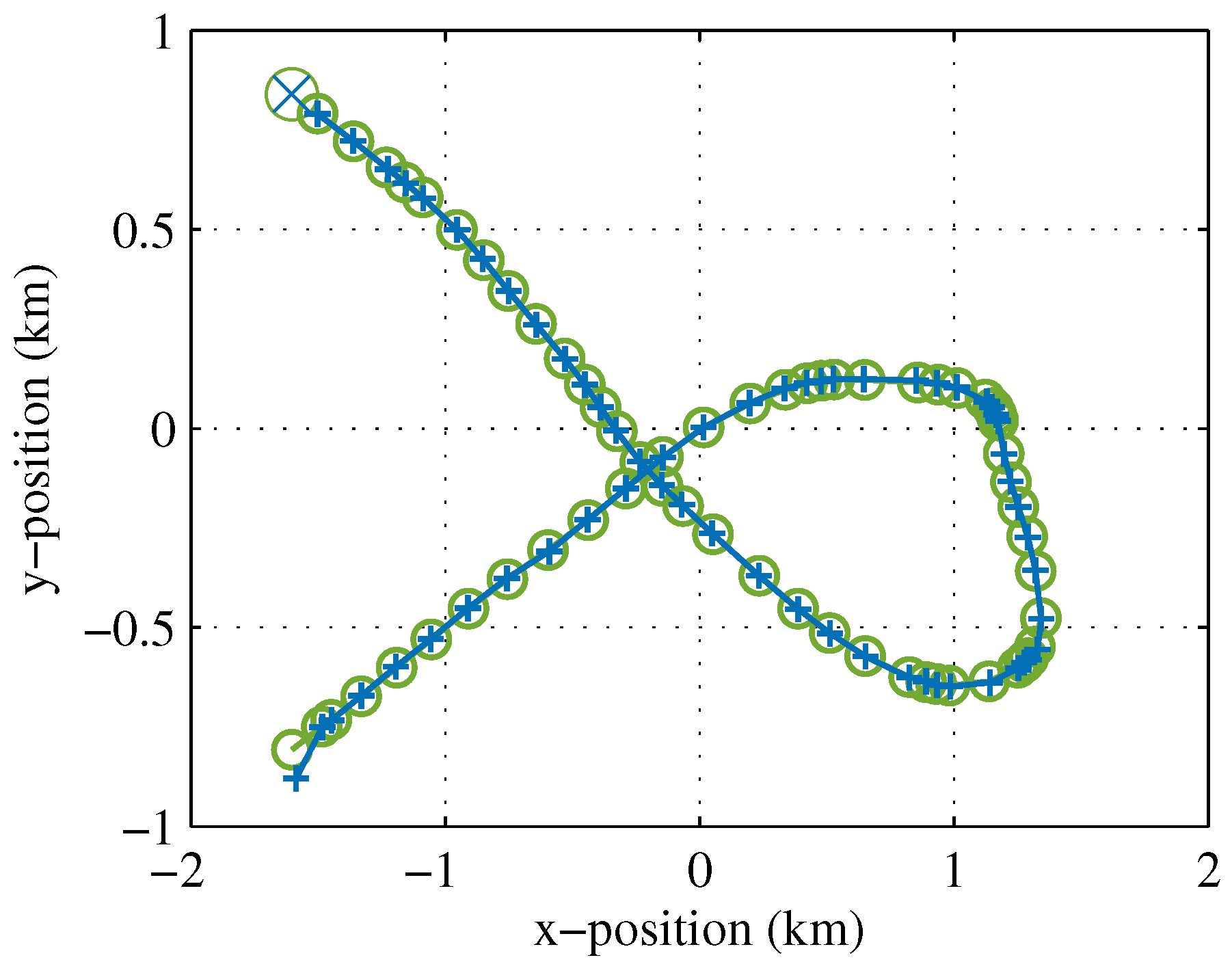
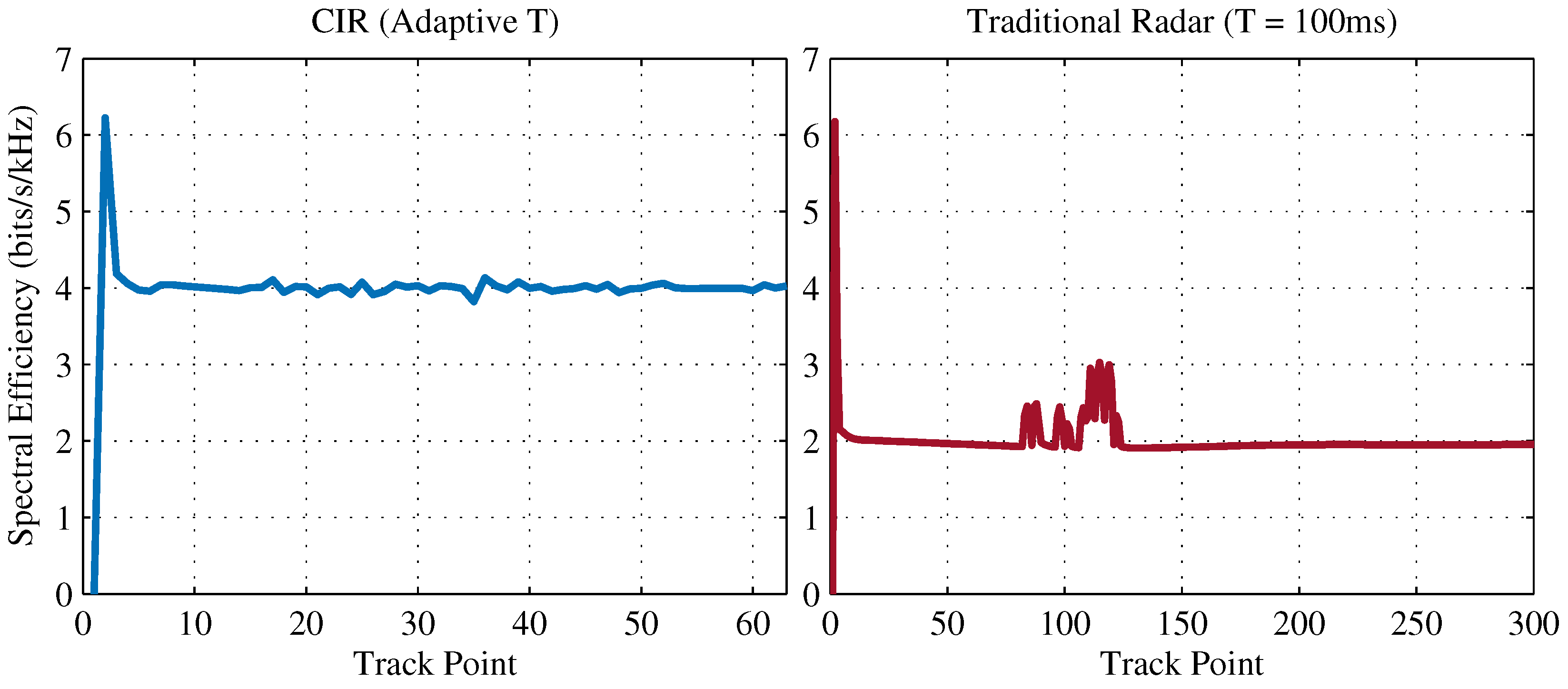
The first track is shown in Figure 8. Note that the plot in Figure 8 is not intended to strictly convey radar tracking performance, but rather to demonstrate the variable revisit time in response to target acceleration. The true track at each observation is shown by the green circle, and the CIR’s estimated track position is shown by the blue crosses. The track was designed to have portions well modeled by the linear, non-accelerative motion model and portions that deviate from this that are captured statistically by the white Gaussian perturbative accelerative noise [42]. In Figure 9, we show the information measure for each track point. The blue plot on the left is the CIR, while the red plot on the right is a traditional radar with fixed revisit time set at 100 ms. For the CIR, the goal is to maintain a constant 10 bits for each target revisit, which provides the minimum number of bits to encode the target position [50]. Taking into account the radar pulse duration, number of pulses, radar duty cycle and radar waveform bandwidth, this corresponds to a spectral efficiency of 4 bits/s/kHz. Since significant redundancy exists from the inclusion of a motion model, only deviations from the model contain information that would need to be encoded. The initial spike larger than 4 bits/s/kHz is due to track acquisition, where the radar detected the target for the first time and obtained a raw measurement with no prior one.

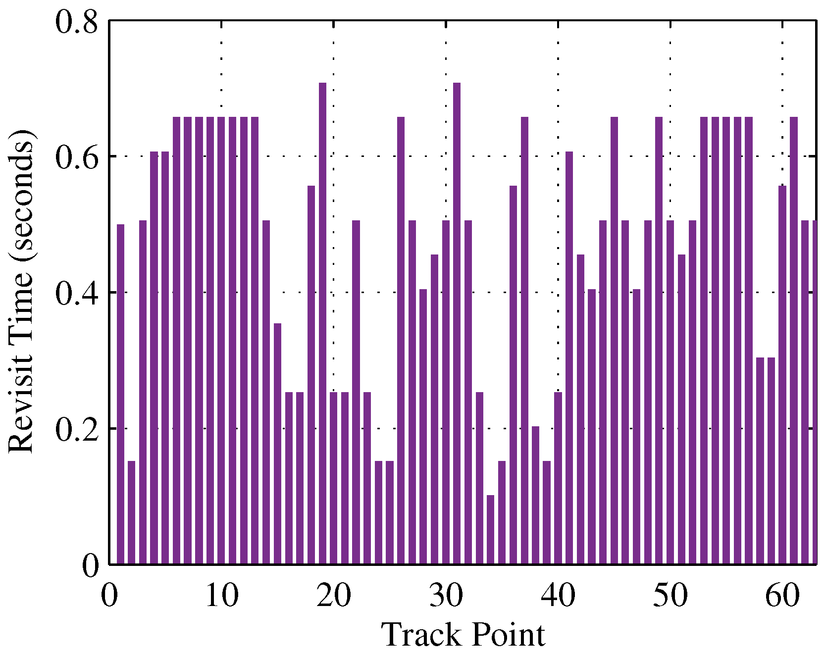
In Figure 10, we see that the time to revisit increases during portions of the track where the target is well modeled. When the target accelerates to turn, the CIR estimates a higher process noise power, and so, more information is predicted to be gained through measurement. As a result, the time between target revisits is decreased. To compare, the same track was simulated using a fixed revisit period of 100 ms. This achieved the same tracking MSE, but with a spectral free time of 99.500% compared to the CIR, which achieved 99.870%. Given the CPI of the radar, this means that the CIR can track nearly 800 targets with similar dynamics compared to the fixed radar’s 200 targets. The spectral efficiency of the fixed radar shown in Figure 9 shows how spectral efficiency fluctuates with changing target dynamics.

Note that the range was chosen to be approximately the same throughout this track, so that SNR did not contribute to the modulation of T significantly. We explore the effect of SNR next by fixing the process noise.

5.2. Approaching Radial Track (SNR Modulation)

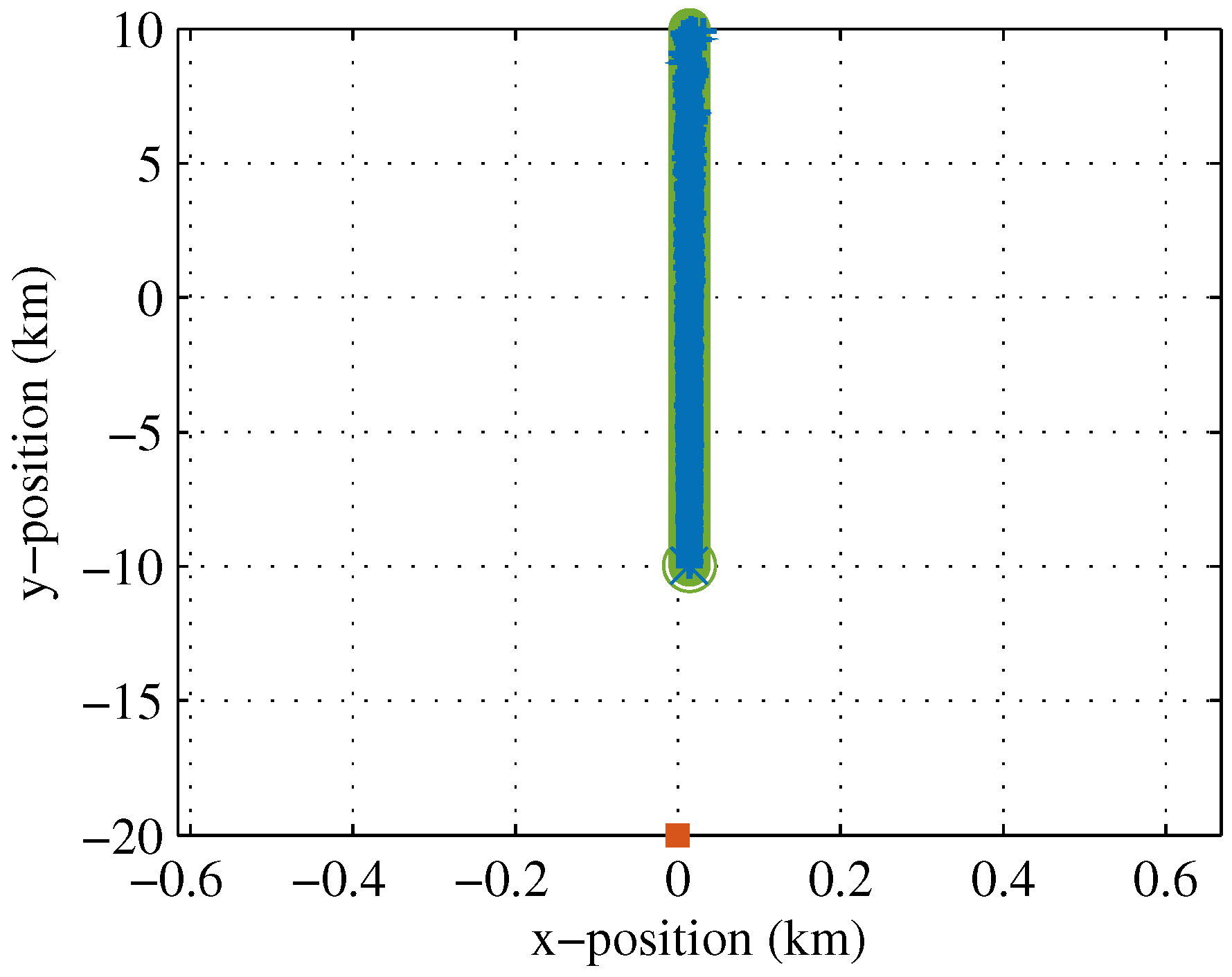
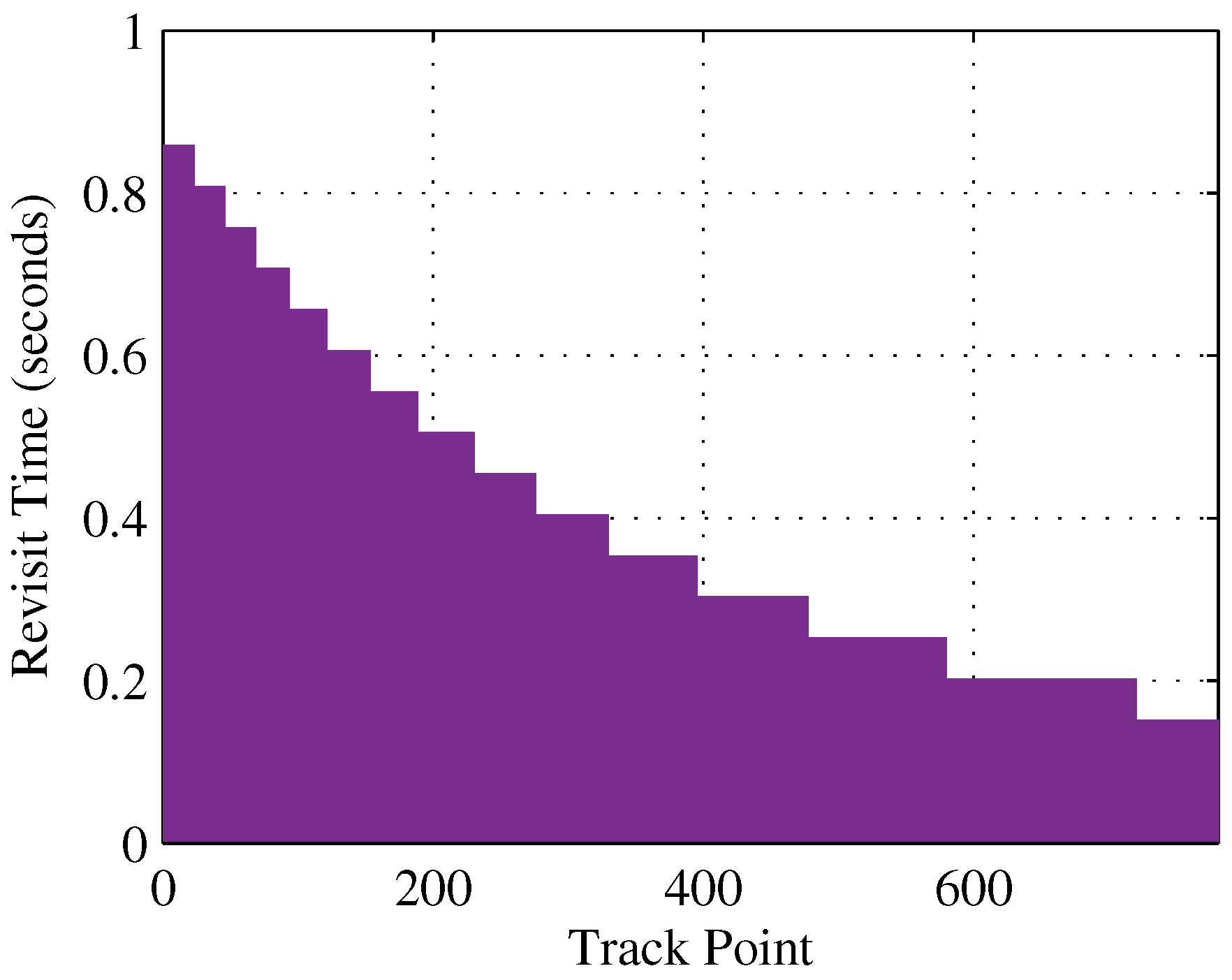
To test a constant process noise, but variable SNR, we simulated an approaching radial track with virtually no acceleration that travels from very far from the radar to very close, as seen in Figure 11. The target revisit time between each track point is shown in Figure 12. When the target is far from the radar, the process noise is swamped by measurement noise. As the target moves toward the radar, much more information stands to be gained from the high SNR. As a result, the actual target information is increased over the same interval, and the revisit time decreases. This curve is similar to one displayed in [33], where compressive sensing based on range is explored.

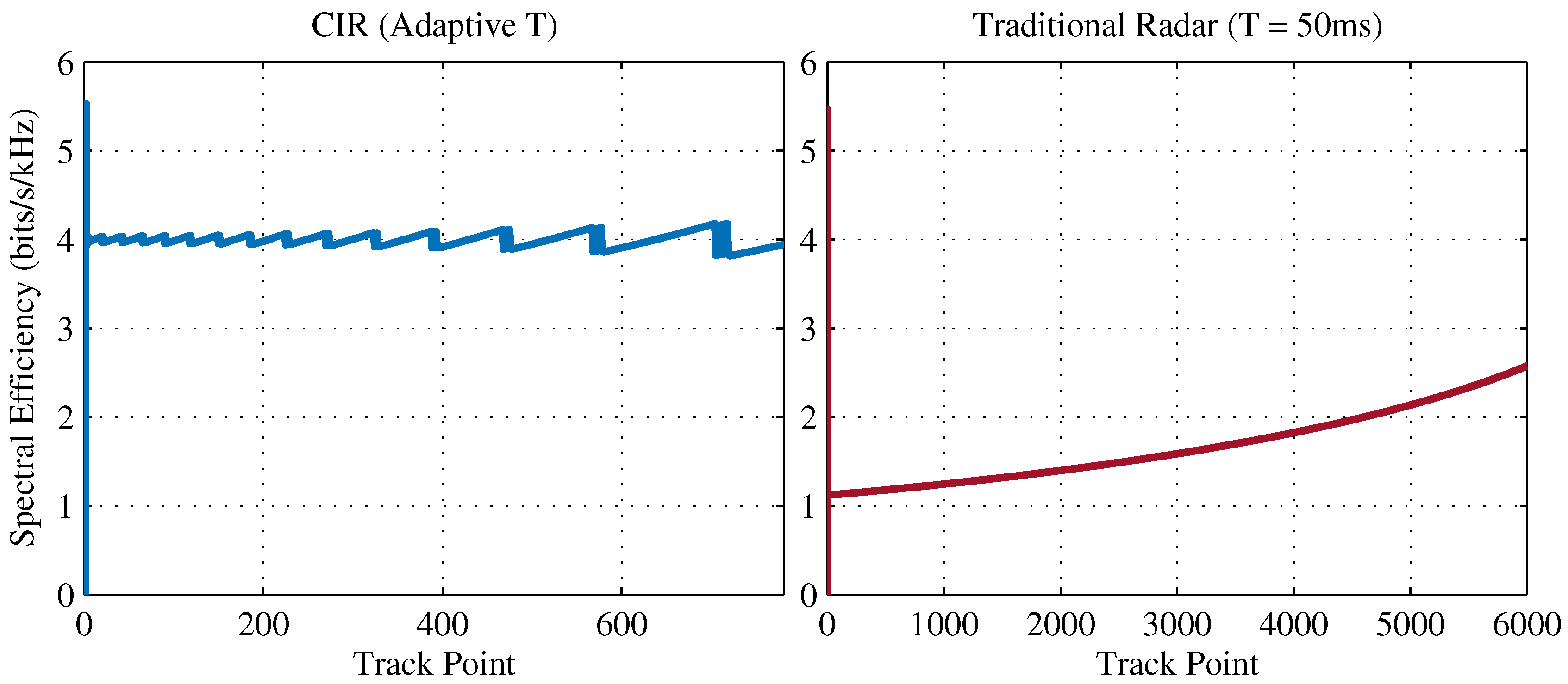
The information plot is shown in Figure 13, where a constant 10 bits was set to be maintained on average (corresponding to a spectral efficiency of 4 bits/s/kHz). Once again, the CIR is on the left in blue, with the fixed radar on the right in red. Note that the quantization of the revisit time lookup table is reflected by the quantization in Figure 12 and results in a sawtooth modulation of the information in Figure 13 for the CIR. To compare, the same track was simulated using a fixed revisit period of 50 ms. This achieved the same tracking MSE, but with a spectral free time of 99.000% compared to the CIR, which achieved 99.834%. Given the CPI of the radar, this means that the CIR can track around 600 targets with similar dynamics compared to the fixed radar’s 100 targets. As the SNR increases, for a fixed revisit time, the spectral efficiency slowly climbs, as shown.

Next, we look at a track that incorporates both global trends (variation in SNR) and local fluctuations due to process noise variance changes.

5.3. Evasive Track (Global and Local Trending)

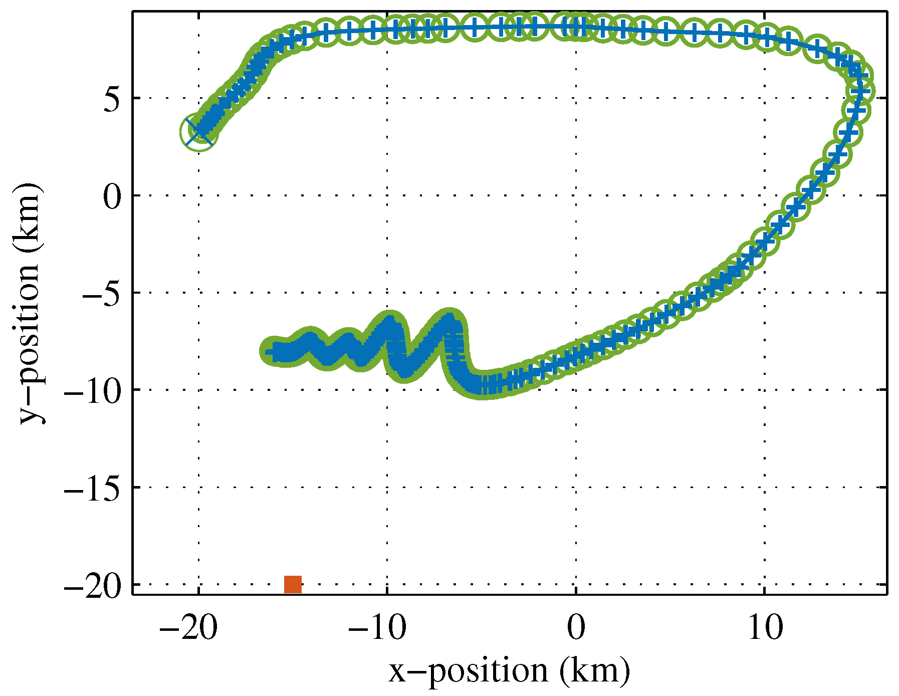
Evasive targets adapt automatically within the entropy framework, as the information content grows with target track uncertainty. A track of an evasive target is shown in Figure 14. In this case, the fixed information value was set at 15 bits to highlight the detail in revisit time modulation.

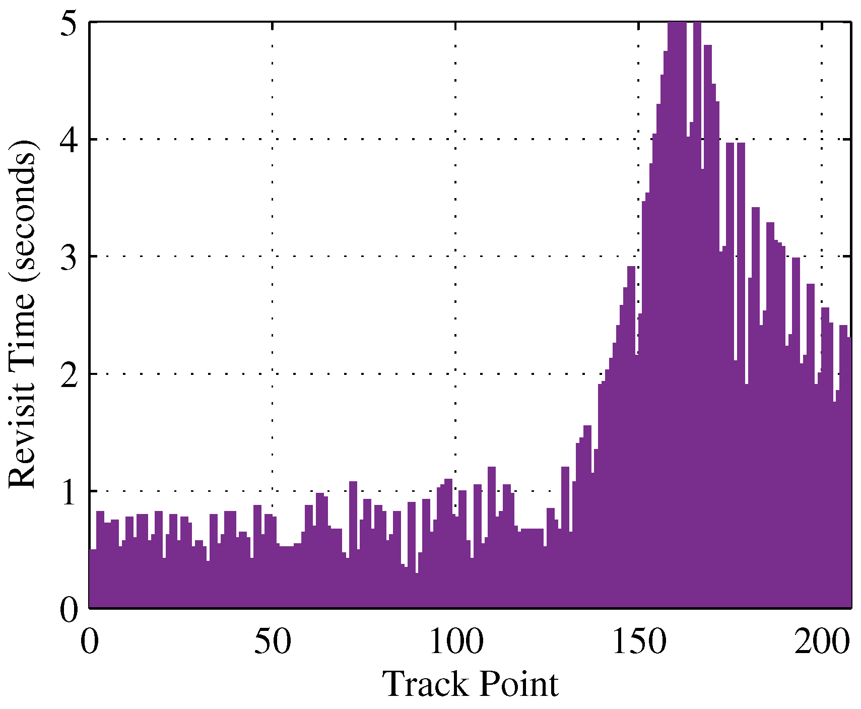
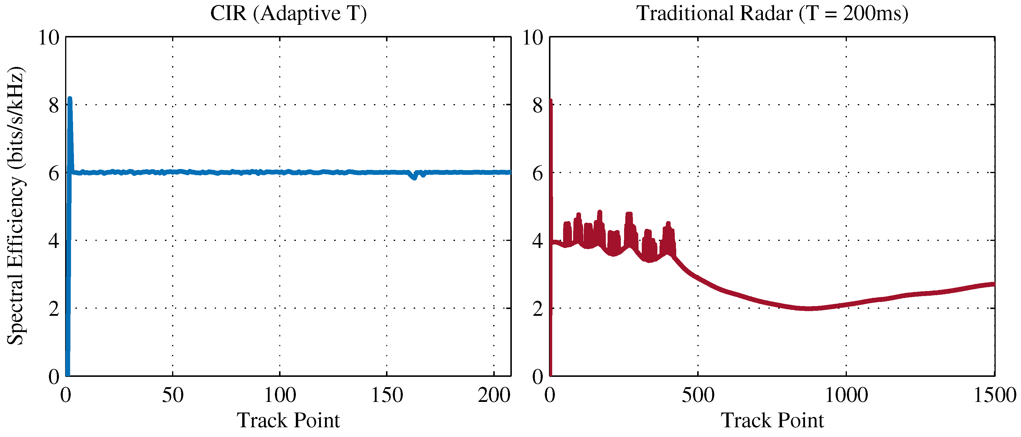
The target revisit time is shown in Figure 15. During the initial period where the target is closer to the radar and attempting to break lock, the radar samples the target much more frequently. The average revisit time is small because of the proximity to the radar, while the small dips in revisit time are during the accelerative turns of the winding behavior. As the target enters linear portions of the track, the radar samples less frequently. Finally, as the target circles around and gets closer to the radar again, the illumination rate is once again starting to increase given the increase in resolution from the growing SNR. The information plot is given by Figure 16, where now we maintain a constant 15 bits of information, or 6 bits/s/kHz. To compare, the same track was simulated using a fixed revisit period of 200 ms. This achieved the same tracking MSE, but with a spectral free time of 99.750% compared to the CIR, which achieved 99.940%. Given the CPI of the radar, this means that the CIR can track almost 1700 targets with similar dynamics compared to the fixed radar’s 400 targets.

In Figure 15, the envelope represents the change in revisit time due to SNR, which is a function of radial distance to the target. Fast variations are due to the process noise variance calculation, which responds instantaneously to deviations in the residual. If averaging were used on the estimation of the process noise to indicate model mismatch, this variation would be less rapid with respect to the track point. The varying spectral efficiency for the fixed radar shown in red in Figure 16 also shows the local and global variation in response to the two target regimes. The results on availability for a traditional radar compared to the CIR for all three track examples are shown in Table 2.

6. Conclusions

We derived the CIR, an information-driven radar that employs a novel algorithm to limit radar spectrum use for dynamic spectrum access. The basic theory of the estimation rate metric was presented, and a model for tracking a target in 2D space was derived. Modulation of the target revisit time as a function of measurement information was discussed to explain the radar behavior. A constant SNR example was given where portions of the track conformed to the motion model, conveying little information. In this same example, sharp turns prompted the CIR to revisit the target more quickly, as target uncertainty increased relative to the tracking model. A radial track with increasing SNR was also presented to illustrate modulation as a function of noise degradation with fixed model mismatch. With SNR increasing as the target traveled closer to the radar, more information from the target measurement was available for a fixed revisit time, and so, the target was revisited more rapidly with the CIR. Finally, a hybrid track with global SNR changes and local process noise variations from accelerative turns showed how the two key dependencies of the CIR scheduling algorithm influence revisit time.

This dynamic time allocation allows for dynamic cooperative sharing with a growing contingent of communications users operating in legacy radar bands. In all examples, the CIR out-performed a traditional radar with a fixed revisit time (chosen such that the average tracking MSE achieved was nearly the same as that achieved by the CIR). The CIR’s increased availability time means that more spectrum access time is possible for in-band cognitive communications users or more targets can be tracked by the CIR.

The CIR concept subsumes the vast model-based tracking phenomenology, so it can be easily generalized to include multiple targets, alternative sensing modalities, complicated clutter and interference distributions and general target tracking distributions. The result is a mathematically-controlled radar with a target scheduling scheme that fixes the radar spectral efficiency for a particular target, ensuring that time-bandwidth is used only when truly needed.

References

- Paul, B.; Bliss, D.W. Constant information radar for dynamic shared spectrum access. In Proceedings of the 49th Asilomar Conference on Signals, Systems and Computers, Pacific Grove, CA, USA, 8–11 November 2015; pp. 1374–1378.
- Bliss, D.W. Cooperative radar and communications signaling: The estimation and information theory odd couple. In Proceedings of the 2014 IEEE Radar Conference, Cincinnati, OH, USA, 19–23 May 2014; pp. 50–55.
- Paul, B.; Bliss, D.W. Extending joint radar-Communications bounds for FMCW radar with Doppler estimation. In Proceedings of the 2015 IEEE Radar Conference, Johannesburg, South Africa, 27–30 October 2015; pp. 89–94.
- Paul, B.; Chiriyath, A.R.; Bliss, D.W. Joint communications and radar performance bounds under continuous waveform optimization: The waveform awakens. In Proceedings of the 2016 IEEE Radar Conference, Philadelphia, PA, USA, 2–6 May 2016; pp. 865–870.
- Chiriyath, A.R.; Bliss, D.W. Joint radar-Communications performance bounds: Data versus estimation information rates. In Proceedings of the 2015 IEEE Military Communications Conference, MILCOM, Tampa, FL, USA, 26–28 October 2015; pp. 1491–1496.
- Chiriyath, A.R.; Bliss, D.W. Effect of clutter on joint radar-Communications system performance inner bounds. In Proceedings of the 49th Asilomar Conference on Signals, Systems and Computers, Pacific Grove, CA, USA, 8–11 November 2015; pp. 1379–1383.
- Chiriyath, A.R.; Paul, B.; Jacyna, G.M.; Bliss, D.W. Inner bounds on performance of radar and communications co-existence. IEEE Trans. Signal Proc. 2016, 64, 464–474. [Google Scholar] [CrossRef]
- Chiriyath, A.R.; Paul, B.; Bliss, D.W. Joint radar-Communications information bounds with clutter: The phase noise menace. In Proceedings of the IEEE Radar Conference, Philadelphia, PA, USA, 2–6 May 2016; pp. 690–695.
- Griffiths, H.; Cohen, L.; Watts, S.; Mokole, E.; Baker, C.; Wicks, M.; Blunt, S. Radar spectrum engineering and management: Technical and regulatory issues. Proc. IEEE 2015, 103, 85–102. [Google Scholar] [CrossRef]
- Chapin, J.M.; Lehr, W.H. Cognitive radios for dynamic spectrum access-the path to market success for dynamic spectrum access technology. IEEE Commun. Mag. 2007, 45, 96–103. [Google Scholar] [CrossRef]
- Bliss, D.W.; Govindasamy, S. Adaptive Wireless Communications: MIMO Channels and Networks; Cambridge University Press: New York, NY, USA, 2013. [Google Scholar]
- Haykin, S. Cognitive radar: A way of the future. IEEE Signal Process. Mag. 2006, 23, 30–40. [Google Scholar] [CrossRef]
- Guerci, J.R.; Guerci, R.M.; Ranagaswamy, M.; Bergin, J.S.; Wicks, M.C. CoFAR: Cognitive fully adaptive radar. In Proceedings of the 2014 IEEE Radar Conference, Cincinnati, OH, USA, 19–23 May 2014; pp. 984–989.
- Sodagari, S.; Khawar, A.; Clancy, T.C.; McGwier, R. A projection based approach for radar and telecommunication systems coexistence. In Proceedings of the IEEE Global Communications Conference (GLOBECOM), Anaheim, CA, USA, 3–7 December 2012; pp. 5010–5014.
- Khawar, A.; Abdel-Hadi, A.; Clancy, T.C. Spectrum sharing between S-band radar and LTE cellular system: A spatial approach. In Proceedings of the IEEE International Symposium on Dynamic Spectrum Access Networks (DYSPAN), McLean, VA, USA, 1–4 April 2014; pp. 7–14.
- Saruthirathanaworakun, R.; Peha, J.M.; Correia, L.M. Opportunistic primary-Secondary spectrum sharing with a rotating radar. In Proceedings of the International Conference on Computing, Networking and Communications (ICNC), Maui, HI, USA, 30 January–2 February 2012; pp. 1025–1030.
- Saruthirathanaworakun, R.; Peha, J.M.; Correia, L.M. Opportunistic sharing between rotating radar and cellular. IEEE J. Sel. Areas Commun. 2012, 30, 1900–1910. [Google Scholar] [CrossRef]
- Setlur, P.; Devroye, N. Adaptive waveform scheduling in radar: An information theoretic approach. In Proceedings of the International Society for Optics and Photonics, Baltimore, MD, USA, 24–26 April 2012.
- Stinco, P.; Greco, M.; Gini, F.; Himed, B. Channel parameters estimation for cognitive radar systems. In Proceedings of the CIP 2014: 4th International Workshop on Cognitive Information Processing, Copenhagen, Denmark, 26–28 May 2014; pp. 1–6.
- Aubry, A.; Maio, A.D.; Naghsh, M.P.M.M.; Soltanalian, M.; Stoica, P. Cognitive radar waveform design for spectral coexistence in signal-dependent interference. In Proceedings of the 2014 IEEE Radar Conference, Cincinnati, OH, USA, 19–23 May 2014; pp. 474–478.
- Paisana, F.; Miranda, J.P.; Marchetti, N.; DaSilva, L.A. Database-Aided sensing for radar bands. In Proceedings of the 2014 IEEE International Symposium on Dynamic Spectrum Access Networks (DYSPAN), McLean, VA, USA, 1–4 April 2014; pp. 1–6.
- Nijsure, Y.; Chen, Y.; Yuen, C.; Chew, Y.H. Location-Aware spectrum and power allocation in joint cognitive communication-Radar networks. In Proceedings of the Sixth International ICST Conference on Cognitive Radio Oriented Wireless Networks and Communications (CROWNCOM), Osaka, Japan, 1–3 June 2011; pp. 171–175.
- Greenspan, M. Potential pitfalls of cognitive radars. In Proceedings of the 2014 IEEE Radar Conference, Cincinnati, OH, USA, 19–23 May 2014; pp. 1288–1290.
- Shannon, C. A mathematical theory of communication. Bell Syst. Tech. J. 1948, 27, 623–656. [Google Scholar] [CrossRef]
- Woodward, P. Information theory and the design of radar receivers. Proc. IRE 1951, 39, 1521–1524. [Google Scholar] [CrossRef]
- Woodward, P.M. Probability and Information Theory, with Applications to Radar; Artech House: Dedham, MA, USA, 1953. [Google Scholar]
- Bell, M.R. Information theory and radar waveform design. IEEE Trans. Inf. Theory 1993, 39, 1578–1597. [Google Scholar] [CrossRef]
- Nijsure, Y.; Chen, Y.; Boussakta, S.; Yuen, C.; Chew, Y.H.; Ding, Z. Novel system architecture and waveform design for cognitive radar radio networks. IEEE Trans. Veh. Technol. 2012, 61, 3630–3642. [Google Scholar] [CrossRef]
- Huang, K.W.; Bică, M.; Mitra, U.; Koivunen, V. Radar waveform design in spectrum sharing environment: Coexistence and cognition. In Proceedings of the 2015 IEEE Radar Conference, Johannesburg, South Africa, 27–30 October 2015; pp. 1698–1703.
- Romero, R.A.; Goodman, N.A. Cognitive radar network: Cooperative adaptive beamsteering for integrated search-and-track application. IEEE Trans. Aerosp. Electron. Syst. 2013, 49, 915–931. [Google Scholar] [CrossRef]
- Hayvaci, H.T.; Tavli, B. Spectrum sharing in radar and wireless communication systems: A review. In Proceedings of the 2014 International Conference on Electromagnetics in Advanced Applications (ICEAA), Palm Beach, Aruba, 3–8 August 2014; pp. 810–813.
- Suvorova, S.; Howard, S.D. Waveform libraries for radar tracking applications: Maneuvering targets. In Proceedings of the 40th Annual Conference on Information Sciences and Systems, Princeton, NJ, USA, 22–24 March 2006; pp. 1424–1428.
- De Jong, E.; Pribić, R. Sparse signal processing on estimation grid with constant information distance applied in radar. EURASIP J. Adv. Signal Process. 2014, 2014, 78. [Google Scholar] [CrossRef]
- Sen, S.; Nehorai, A. Sparsity-based multi-target tracking using OFDM radar. IEEE Trans. Signal Process. 2011, 59, 1902–1906. [Google Scholar] [CrossRef]
- Akcakaya, M.; Sen, S.; Nehorai, A. A novel data-driven learning method for radar target detection in nonstationary environments. IEEE Signal Process. Lett. 2016, 23, 762–766. [Google Scholar] [CrossRef]
- Romero, R.A.; Bae, J.; Goodman, N.A. Theory and application of SNR and mutual information matched illumination waveforms. IEEE Trans. Aerosp. Electron. Syst. 2011, 47, 912–927. [Google Scholar] [CrossRef]
- Watson, G.A.; Blair, W.D. Revisit calculation and waveform control for a multifunction radar. In Proceedings of the 32nd IEEE Conference on Decision and Control, San Antonio, TX, USA, 15–17 December 1993; pp. 456–460.
- Alahmadi, M.S.; Smith, G.E.; Baker, C.J. A recursive approach for adaptive parameters selection in a multifunction radar. In Proceedings of the 2016 IEEE Radar Conference, Philadelphia, PA, USA, 2–6 May 2016; pp. 1–6.
- Guerci, J.R.; Guerci, R.M.; Lackpour, A.; Moskowitz, D. Joint design and operation of shared spectrum access for radar and communications. In Proceedings of the IEEE Radar Conference, Johannesburg, South Africa, 27–30 October 2015; pp. 761–766.
- Reed, J.T.; Odom, J.L.; Causey, R.T.; Lanterman, A.D. Gaussian multiple access channels for radar and communications spectrum sharing. In Proceedings of the IEEE Radar Conference, Philadelphia, PA, USA, 2–6 May 2016; pp. 1–6.
- Turlapaty, A.; Jin, Y. A Joint design of transmit waveforms for radar and communications systems in coexistence. In Proceedings of the IEEE Radar Conference, Cincinnati, OH, USA, 19–23 May 2014; pp. 315–319.
- Li, X.R.; Jilkov, V.P. Survey of maneuvering target tracking. Part I: Dynamic models. Trans. Aerosp. Electron. Syst. 2003, 39, 1333–1364. [Google Scholar]
- Richards, M.A. Fundamentals of Radar Signal Processing, 2nd ed.; McGraw-Hill Education: Raleigh, NC, USA, 2014. [Google Scholar]
- Richards, M.A. Principles of Modern Radar: Basic Principles; SciTech Publishing: Raleigh, NC, USA, 2010. [Google Scholar]
- Van Trees, H.L. Detection, Estimation, and Modulation Theory: Radar-Sonar Signal Processing and Gaussian Signals in Noise; Krieger Publishing Company: Malabar, FL, USA, 1992. [Google Scholar]
- Candy, J.V. Bayesian Signal Processing: Classical, Modern, and Particle Filtering Methods; John Wiley & Sons: Hoboken, NJ, USA, 2009. [Google Scholar]
- Richmond, C.D. Mean-squared error and threshold SNR prediction of maximum-likelihood signal parameter estimation with estimated colored noise covariances. Trans. Inf. Theory 2006, 52, 2146–2164. [Google Scholar] [CrossRef]
- Paul, B.; Bliss, D.W. Estimation information bounds using the I-MMSE formula and Gaussian mixture models. In Proceedings of the 50th Annual Conference on Information Sciences and Systems (CISS), Princeton, NJ, USA, 16–18 March 2016; pp. 292–297.
- Kay, S.M. Fundamentals of Statistical Signal Processing: Estimation Theory, 1st ed.; Prentice-Hall: Upper Saddle River, NJ, USA, 1993. [Google Scholar]
- Cover, T.M.; Thomas, J.A. Elements of Information Theory, 2nd ed.; John Wiley & Sons: Hoboken, NJ, USA, 2006. [Google Scholar]
- Davey, S.J.; Rutten, M.G.; Cheung, B. A comparison of detection performance for several Track-Before-Detect algorithms. In Proceedings of the 11th International Conference on Information Fusion, Cologne, Germany, 30 June–3 July 2008; pp. 1–8.
- Myers, K.A.; Tapley, B.D. Adaptive sequential estimation with unknown noise statistics. Trans. Autom. Control. 1976, 21, 520–523. [Google Scholar] [CrossRef]
Figure 1.
Top level view of the constant information radar (CIR) scheduling concept. At the Kalman prediction step, the predicted SNR and model covariance are used to predict the tracking mutual information. If the predicted information is smaller than some configured value, , then the revisit time is increased. Conversely, the revisit time is decreased if the predicted information exceeds this value, indicating greater than desired uncertainty. This modulation ensures a fixed spectral efficiency for the radar and precludes unnecessary sampling of well-modeled targets or targets that are obfuscated by noise or clutter beyond target state uncertainty.
Figure 2.
Illustration of the target motion model. The previous measurement is indicated by the solid gray plane. The positional covariance contour is shown surrounding the plane, while the velocity vector leading the plane has a covariance as well to indicate the degree of confidence in the current target state. Using a constant velocity model, the prediction shown by the dashed lines is made by advancing the target in time as if the last state were the truth, and the plane is not accelerating. Since the plane can, in fact, accelerate and because we had an initial uncertainty about the state, the prediction covariance shown in the dashed contours is increased.
Figure 3.
Measurement model showing Cartesian to polar transformation. While we track the target in Cartesian space to avoid coordinate-coupled physics, we measure waveform echo delay, Doppler shift and bearing angle. From the delay and bearing, a direct polar transformation can recover the 2D position. However, the velocity vector is only projected along the radial axis through the Doppler effect (range-rate), meaning multiple measurements and position history are needed to unambiguously recover velocity.
Figure 4.
Illustration of prediction compared to measurement with a low entropy and ultimately low information target. Predictions at each track point are represented by the dashed outlines. Actual measurements are shown in the filled-gray planes. The last track point shows the prediction and model mismatch covariance or uncertainty contour. In this illustration, our constant velocity model is well matched to the benign target. As a result, the deviation from prediction at each measurement is small, and for a fixed revisit period as illustrated here, little information is learned through spectral use.
Figure 5.
Illustration of prediction compared to measurement with a high entropy and ultimately high information target. Predictions at each track point are represented by the dashed outlines. Actual measurements are shown in the filled-gray planes. The last track point shows the prediction and model mismatch covariance or uncertainty contour. In this illustration, our constant velocity model is poorly matched to the dynamic target executing a serpentine maneuver. As a result, the deviation from prediction at each measurement is larger, and for a fixed revisit period as illustrated here, significant information is learned through spectral use.
Figure 6.
Illustration of measurement variance in contrast to the mean residual. The prediction is indicated by the blue-filled plane with the dashed outline. The swarm of gray planes with the solid outline represents multiple measurements at the same track point. Each time a measurement is made over the ensemble, it is perturbed uniquely by either clutter, noise or interference. In the high SNR case on the left, the perturbations are small, and the grouping is tight. As a result, the mean offset from the prediction is significant and appreciable. For the low SNR case to the right, the offset of the mean to the prediction is insignificant compared to the variance of the measurement indicated by the degree of spread in these samples. As a result, low information gain is possible compared to the high SNR case.
Figure 7.
Motivation of delayed revisit time in response to poor SNR. The prediction is indicated by the blue-filled plane with the dashed outline. The swarm of gray planes with the solid outline represents multiple measurements at the same track point. Each time a measurement is made over the ensemble, it is perturbed uniquely by either clutter, noise or interference. For low SNR, the offset of the mean to the prediction is insignificant compared to the variance of the measurement indicated by the degree of spread in these samples shown on the left. By increasing the revisit time, the model uncertainty grows larger, and the offset from the prediction can grow to become significant relative to the variance of the measurement. As a result, significant information is recovered, and spectral efficiency is increased.
Figure 8.
Example of a looping track with realization overlay. The green circles indicate the true target position at each time step (indicated by the markers). The blue crosses indicate the CIR’s estimated target position. In the straight portions of the track, the target is not accelerating and is adhering to the predicted model well. During the curved parts of the track, the target is necessarily accelerating, and as a result, the CIR revisits the target more frequently over an equivalent time period.
Figure 9.
Spectral efficiency at each track point given in bits/s/kHz for the looping track. On the left, in blue, is the CIR, which modulates the radar target revisit period in response to information. The goal was to maintain 10 bits of information or 4 bits/s/kHz with this radar configuration. Initial uncertainty during track acquisition resulted in a larger spike. Subsequently, the revisit time is modulated to maintain 10 bits. On the right, in red, is a traditional radar with a fixed revisit time. Spectral efficiency fluctuates in response to changing target dynamics.
Figure 10.
Target revisit time at each track point given in seconds (time between each track points) for the looping track. During turns where more information stands to be gained, the target is revisited faster. When the target is well-modeled (and little information stands to be gained), the revisit time is increased, allowing for more radar-free spectrum access or tracking of additional targets.
Figure 11.
Example of an approaching radial track with realization overlay; the radar position is represented as an orange block. The green circles indicate the true target position at each time step, while the blue crosses indicate the CIR estimated target position. Since the track is linear and the target is not accelerating along this line, the constant velocity model is a good match to the target dynamics. However, the radius from the radar is decreasing linearly with time, and so, the SNR is increasing with time. As a result, the track is sampled more frequently by the CIR as time progresses.
Figure 12.
Target revisit time at each track point given in seconds for the approaching radial track with increasing SNR. Since the SNR is increasing as the radial distance decreases, the information content is increasing for a fixed revisit time. As a result, the revisit time is decreased as the track progresses to keep the information constant.
Figure 13.
Spectral efficiency at each track point given in bits/s/kHz for the approaching radial track with increasing SNR. On the left, in blue, is the CIR, which modulates the radar target revisit period in response to information. The CIR was set to maintain 10 bits or 4 bits/s/kHz for this scenario. Ripples are from quantization due to the finite number of available revisit times in the lookup table described in Algorithm 1 derived in Section 3.2. On the right, in red, is a traditional radar with a fixed revisit time. Spectral efficiency increases steadily in response to increasing SNR as the target approaches the radar location.
Figure 14.
Example of an evasive track with realization overlay; the radar position is indicated by the orange block. The green circles once again indicate the true target position at each time step, and the blue crosses show the CIR’s estimated target position. Initially, the target executes an evasive serpentine maneuver, and the CIR reacts appropriately by revisiting the target more frequently. As the target moves significantly far away from the radar, the decaying SNR forces the CIR to sample less often.
Figure 15.
Target revisit time at each track point given in seconds for an evasive track. During the initial maneuver, the target is in nearly constant acceleration, and so, the revisit time is very short on average. The target then slowly eases into a linear constant velocity straight-away, and the CIR revisits the target less frequently. As the target rounds a turn, there are periods where the target is sampled more often before it is again well modeled. There is a clear global trend overlaid on the local trend. The global envelope of the revisit time plot is due to SNR and fluctuates with radial distance. Locally, the dips and peaks comprising this envelope are due to periods of acceleration or turning since the process noise variance is calculated every track point.
Figure 16.
Spectral efficiency at each track point given in bits/s/kHz for an evasive track. On the left, in blue, is the CIR, which modulates the radar target revisit period in response to information. The CIR was set to maintain 15 bits or 6 bits/s/kHz. On the right, in red, is a traditional radar with a fixed revisit time. Spectral efficiency fluctuates in response to changing target dynamics, as well as SNR varying slowly in response to target location relative to the radar.