A Probabilistic Damage Identification Method for Shear Structure Components Based on Cross-Entropy Optimizations

Abstract

A probabilistic damage identification method for shear structure components is presented. The method uses the extracted modal frequencies from the measured dynamical responses in conjunction with a representative finite element model. The damage of each component is modeled using a stiffness multiplier in the finite element model. By coupling the extracted features and the probabilistic structural model, the damage identification problem is recast to an equivalent optimization problem, which is iteratively solved using the cross-entropy optimization technique. An application example is used to demonstrate the proposed method and validate its effectiveness. Influencing factors such as the location of damaged components, measurement location, measurement noise level, and damage severity are studied. The detection reliability under different measurement noise levels is also discussed in detail.

1. Introduction

The ability to identify a damaged component in aerospace, mechanical, and civil systems is becoming increasingly important [1,2,3]. Although extensive efforts have been devoted in the diagnostics and prognostics community to develop effective methods for damage diagnostics and identifications over the past few decades, structural damage identification is still regarded as a practical challenge for safety assurance of engineering structures [4,5]. A widely-used classification system for damage diagnosis defines four levels of damage identifications: the first level is to determine the existence of the damage in the structure; the second level is to obtain the geometric location of the damage; the third level is to quantify the severity of the damage; and the fourth level is to estimate the remaining useful life of the structure [6]. Damage quantification usually focuses on the first three levels, and the fourth level is generally related to life prediction methods involving damage evolution mechanisms.

Several non-destructive evaluation methods such as ultrasound inspection [7,8,9,10,11,12,13], eddy-current testing [14,15], and Lamb wave-based methods [16,17,18,19,20,21] can effectively identify local damages in a component. To identify the component damage on a global basis, capturing the changes in vibration characteristics of the entire structure is one of the few methods that can be applied in practice [22,23]. A review on using modal frequency changes for damage identification can be found in [24]. Ref. [25] provided a formulation to detect damage in composite materials using frequency shifts. The method uses measurements of changes in the lower structural natural frequencies that are made at a single point in the structure in conjunction with a dynamic analysis of the system to detect the damage. The advantage of the method is that natural frequency and damping ratio can be obtained using measurement at a single point on the structure, and they are independent of the chosen measurement position; however, it requires a sufficiently accurate dynamic analysis of the structure to obtain mode shapes for estimation of damage location and severity. Friswell et al. [26] reported a method to identify damage based on a known catalog of possible damage scenarios and an accurate structural model using a two-step process. The first step computes frequency shifts of the first several modes for both the undamaged structure and all the possible damage scenarios. The second step uses the ratios of all frequency shifts to fit a power-law model for damage scenario identification. Fritzen et al. [27] developed a damage detection method based on model updating concept and applied the method to a numerical cracked beam and a damaged rectangular metal plate. The idea is to use a mathematical model representing the undamaged vibrating structure and a local description of the damage. For a damage localization to be successful, the reference finite element model must be as accurate as possible; otherwise, the procedure will lead to incorrect results. Bayissa et al. [28] proposed a damage identification method using wavelet transformation and applied the method to a steel plate girder of a bridge for damage identification. Deraemaeker et al. [29] developed a structural health monitoring process using vibration data. The process extracts the eigenproperties of the structure and the peak indicators computed on the Fourier transform of modal filters, and use them as damage indicators. The method can identify the existence of the damage in the structure, but it is difficult to accurately estimate the damage location. Fugate et al. [30] reported a direct time domain method for damage detection using pattern recognition techniques. The method uses an auto-regressive (AR) model to fit the vibration time series, and the difference between the AR model prediction and the actual vibration time series of the damaged system is used as a damage feature. If excitation sources and/or environmental conditions change, it is very difficult for the identification using direct time series to produce reliable results, and it is even more difficult to relate the time series changes to physical changes in the structure [31]. Although most of the aforementioned methods are deterministic, the identification of structural damage is a nondeterministic problem in nature due to inherent modeling and measurement uncertainties. The identification using deterministic methods may lead to faulty conclusions of structural damages (i.e. false positives of damages) [32]. More importantly, probabilistic methods can provide uncertainty quantification and management for risk mitigation. For nondeterministic approaches, Bayesian structural model identification and damage detection methods using output only dynamical responses have been systematically studied by Beck and his colleagues [33,34,35,36]. Friswell and Mottershead [37] provided a comprehensive reference for finite model updating using structural dynamics data. More survey studies on Bayesian model updating for structural damage identification can be found in [31,38,39]. The central idea is to update the initial distribution of model parameters using measured data. The model parameters can be stiffness, mass, and damping in a finite element context. It usually requires multiple and continuous updates to obtain reliable results when prior information is limited. The posterior probability density functions (PDFs) are usually obtained using Markov chain Monte Carlo simulations, and is not designed for real-time operations.

The objective of this study is to develop an efficient probabilistic damage identification method for shear structural components with a minimal set of measurement data. The proposed method uses dynamical response measurement data obtained under random loading in conjunction with a representative finite element model. The damage of a component is encoded in the model by a stiffness multiplier applied to the nominal value. The dynamical response measurement data are used to extract the actual modal frequencies of the structure statistically. The stiffness multiplier is modeled using a truncated normal distribution in the range of (0,1] with an initial mean value of 0.5 and a constant standard deviation. A set of multipliers are randomly generated to formulate a set of test structural models. Calculated modal frequencies of test models are compared with the extracted modal frequencies from measurement data through a performance function. The damage identification problem is recast to a probabilistic optimization problem, which is then solved using cross-entropy optimization algorithms. The paper is organized as follows. First, the basic concept of the cross-entropy optimization technique is briefly introduced. Next, the probabilistic damage identification for a general structure is formulated based on the cross-entropy optimizations, and the generic algorithm is described. The iterative updating scheme for the distribution parameter of the stiffness multiplier is derived for the truncated normal distribution. Following that, a shear structure example is used to demonstrate and validate the overall method. Influences from damage location, measurement location, measurement noise, and damage severity are studied using four damage cases generated by the Latin hypercube design method. The reliability of the proposed method in terms of probability of detection is also investigated under different measurement noise conditions.

2. General Cross-Entropy Optimization

The cross-entropy optimization method is developed in the filed of rare event simulation and is pioneered by Rubinstein and others [40,41,42]. The original cross-entropy method is used to find the optimal importance sampling density. The method later evolves to a unified simulation-based optimization method by recasting the optimization problem to an associated stochastic problem. The method involves a two-step iteration process that is particularly suitable for computer implementations. The two-step procedure is described as follows:

• Generate a random set of candidate states of the system according to a specified mechanism.
• Rank the candidate states based on particular performance measures and keep candidate states that perform well and use them for the next iteration. This step usually involves minimization of the cross-entropy measure.

For completeness purposes, the basic idea of cross-entropy method is briefly introduced. Denote $X=\{X_1,X_2,...,X_k\}$ as a k-dimensional random variable taking values in $\mathcal{X}$ and having a probability distribution of $f(x;\theta )$, where θ is the distribution parameter. Define a real-valued function $h\left(x\right)$, and the probability of $h\left(x\right)\ge \gamma$ is of interest. The probability can be expressed as

$$l_{\theta }={\int }_{h\left(x\right)\ge \gamma }f(x;\theta )\mathrm{d}x={\mathbb{E}}_f\left[\mathbf{1}\left(h\right(X)\ge \gamma )\right],$$

(1)

where $\mathbf{1}\left(h\right(x)\ge \gamma )$ is the indicator function taking value of 1 if $h\left(x\right)\ge \gamma$, and 0 otherwise. ${\mathbb{E}}_f\left[·\right]$ is the expectation operator under the distribution $f(x;\theta )$. For realistic problems, $l_{\theta }$ is usually estimated using simulation-based methods, such as Monte Carlo (MC) method or its variants. According to the Law of Large Numbers and the Central Limit Theorem, the MC estimator has a relative error of

$$ϵ\approx \frac{1}{\sqrt{N{l}_{\theta }}},$$

(2)

where N is the number of simulation samples. If $l_{\theta }$ is very small (rare event), for example $l_{\theta }={10}^{-6}$ and $ϵ=0.01$, the estimator needs $N\approx {10}^{10}$ samples, which is computationally infeasible. The important sampling (IS) method uses a different distribution $g\left(x\right)$ to draw samples, and $l_{\theta }$ can be estimated as

$$l_{\theta }={\int }_{h\left(x\right)\ge \gamma }\frac{f(x;\theta )}{g\left(x\right)}g\left(x\right)\mathrm{d}x={\mathbb{E}}_g\left[\mathbf{1}(h\left(X\right)\ge \gamma )\frac{f(X;\theta )}{g\left(X\right)}\right].$$

(3)

It is seen that the ideal $g\left(x\right)$, denoted as $g_{*}\left(x\right)$, is

$$g_{*}\left(x\right)=\frac{\mathbf{1}\left(h\right(x)\ge \gamma )f(x;\theta )}{l_{\theta }}.$$

(4)

By using the change of measure in Equation (4), the following result is guaranteed

$$\mathbf{1}(h(X^{\left(i\right)})\ge \gamma )\frac{f(X^{\left(i\right)};\theta )}{g_{*}\left(X^{\left(i\right)}\right)}=l_{\theta },\forall i\in 0,1,\cdots ,N,$$

(5)

where $X^{\left(i\right)}$ is the $i\mathrm{th}$ random sample. This means the estimator has zero variance and only $N=1$ sample is needed. However, $g_{*}\left(x\right)$ is difficult to obtain because $l_{\theta }$ is unknown. Therefore, it is desired to find a $g\left(x\right)$ which is as close to the ideal distribution of Equation (4) as possible. In practice, $g\left(x\right)$ can be chosen as the same type of distribution as $f(x;\theta )$ but with a different parameter $\tilde{\theta }$, i.e., $g\left(x\right):=f(x;\tilde{\theta })$. One of the convenient measures for “distance” between two distributions is the Kullback–Leibler (KL) distance [43], which is also referred as cross-entropy in engineering and is defined as

$$\mathbb{H}(p_1,p_2)={\int }_{\mathcal{X}}{p}_1\left(x\right)ln\frac{p_1\left(x\right)}{p_2\left(x\right)}\mathrm{d}x={\mathbb{E}}_{p_1}\left[ln\frac{p_1\left(X\right)}{p_2\left(X\right)}\right],$$

(6)

where $p_1\left(x\right)$ and $p_2\left(x\right)$ are two distributions. Minimization of Equation (6) between $g_{*}\left(x\right)$ and $g\left(x\right):=f(x;\tilde{\theta })$ leads to minimizing

$${\mathbb{E}}_{\tilde{\theta }}\left[ln\frac{g_{*}\left(X\right)}{f(X;\tilde{\theta })}\right]=\sum _x{g}_{*}\left(x\right)ln{g}_{*}\left(x\right)-\sum _x{g}_{*}\left(x\right)lnf(x;\tilde{\theta }),$$

(7)

which is equivalent to maximizing ${\sum }_x{g}_{*}\left(x\right)lnf(x;\tilde{\theta })$ due to the fact that ${\sum }_x{g}_{*}\left(x\right)ln{g}_{*}\left(x\right)$ is a constant. Substitution of $g_{*}\left(x\right)$ from Equation (4) into Equation (7) casts the problem to finding

$${\theta }_{*}=\underset{\tilde{\theta }}{arg\; max}{\mathbb{E}}_{\theta }\left[\mathbf{1}(h\left(X\right)\ge \gamma )f(X;\theta )lnf(X;\tilde{\theta })\right].$$

(8)

Given an initial sampling distribution $f(x;{\theta }_0)$, Equation (8) is equivalent to

$${\theta }_{*}=\underset{\tilde{\theta }}{arg\; max}{\mathbb{E}}_{{\theta }_0}\left[\mathbf{1}(h\left(X\right)\ge \gamma )W(X;\theta ,{\theta }_0)lnf(X;\tilde{\theta })\right],$$

(9)

where $W(x;\theta ,{\theta }_0)=\frac{f(x;\theta )}{f(x;{\theta }_0)}$ is the likelihood ratio. Using discrete samples, ${\theta }_{*}$ can be estimated by

$${\widehat{\theta }}_{*}=\underset{\tilde{\theta }}{arg\; max}\sum _{i=1}^N\mathbf{1}(h(X^{\left(i\right)})\ge \gamma )W(X^{\left(i\right)};\theta ,{\theta }_0)lnf(X^{\left(i\right)};\tilde{\theta }),$$

(10)

where $X^{\left(1\right)},X^{\left(2\right)},...,X^{\left(N\right)}$ are random samples from $f(x;{\theta }_0)$. ${\widehat{\theta }}_{*}$ can be obtained by solving the following equations

$$\sum _{i=1}^N\mathbf{1}(h(X^{\left(i\right)})\ge \gamma )W(X^{\left(i\right)};\theta ,{\theta }_0)\nabla lnf(X^{\left(i\right)};{\widehat{\theta }}_{*})=0.$$

(11)

Given that the distribution of $f(x;\tilde{\theta })$ belongs to a natural exponential family, ${\widehat{\theta }}_{*}$ can be calculated analytically. An iterative procedure of solving ${\theta }_{*}$ is presented as Algorithm 1 [40].

Algorithm 1 Iterative Procedure of Estimation for ${\theta }_{*}$

$t\leftarrow 0$, initialize ${\theta }_0$, e.g., ${\theta }_0=\theta$.  repeat   (1) Draw N random samples $x^{\left(1\right)},x^{\left(2\right)},...,x^{\left(N\right)}$ from $f(x;{\theta }_t)$.   (2) Calculate $h_i=h(x^{\left(i\right)})$ for all i. Sort $h_i$ from largest to smallest.   (3) ${\gamma }_t\leftarrow h_M$, where $1\le M\le N$.   (4) Calculate ${\theta }_{t+1}$ by solving ${\sum }_{i=1}^N\mathbf{1}(h(X^{\left(i\right)})\ge \gamma )W(X^{\left(i\right)};\theta ,{\theta }_t)\nabla lnf(X^{\left(i\right)};{\theta }_{t+1})=0$.   (5) $t\leftarrow t+1$.  until ${\gamma }_t\ge \gamma$.  ${\theta }_{*}\leftarrow {\theta }_{t+1}$.

For optimization problems, Algorithm 1 needs slight modifications because the objective is not finding an optimized important sampling distribution parameter ${\theta }_{*}$. The idea is to convert an optimization problem to its associated stochastic problem. Consider a general minimization problem with a real-valued performance function $h\left(x\right)$ and a state variable $x\in \mathcal{X}$. The minimum of $h\left(x\right)$ is denoted as ${\gamma }_{*}$ when x is equal to $x_{*}$. Define a threshold value $\gamma \in \mathbb{R}$ and an indicator function $\mathbf{1}\left(h\right(x)\le \gamma )$. This setting allows one to estimate the probability of $h\left(x\right)\le \gamma$ as

$$\begin{array}{cc}\hfill l_{\theta }\left(\gamma \right)& ={\int }_{h\left(x\right)\ge \gamma }\mathbf{1}(h\left(x\right)\le \gamma )f(x;\theta )\mathrm{d}x={\mathbb{E}}_{\theta }\left[\mathbf{1}\left(h\right(x)\le \gamma )\right]\hfill \\ & =\sum _x\mathbf{1}(h\left(x\right)\le \gamma )f(x;\theta ),\hfill \end{array}$$

(12)

where $f(x;\theta )$ is defined as before. It is seen that if γ is close to ${\gamma }_{*}$, i.e., $\gamma ={\gamma }_{*}+ϵ$, where ϵ is a very small positive, $h\left(x\right)\le \gamma$ can be treated as a rare event. In that case, $l_{\theta }({\gamma }_{*}+ϵ)$ will be a small quantity and thus the important sampling can be used to estimate it efficiently. The ideal parameter ${\theta }_{*}$ of the important sampling distribution $f(x;{\theta }_{*})$ can be estimated following Equations (8)–(11) as

$$\sum _{i=1}^N\mathbf{1}(h(X^{\left(i\right)}\le \gamma ))\nabla lnf(X^{\left(i\right)};{\theta }_{*})=0.$$

(13)

The term $W(X^{\left(i\right)};\theta ,{\theta }_0)$ is dropped out from Equation (13) because, in each iteration, ${\gamma }_t$ is assigned a new value based on samples of the current iteration. As a result, the corresponding θ is equal to ${\theta }_t$ and $W(X;\theta ,{\theta }_t)=1$. The correlation between the estimation of $l_{\theta }({\gamma }_{*}+ϵ)$ and finding the solution to the optimization problem (i.e., $x_{*}$) lies in the following fact: it is plausible that $f(x;{\theta }_{*})$ assigns most of its probability mass close to $x_{*}$ if γ is close to ${\gamma }_{*}$; therefore, the resulting simulation samples from $f(x;{\theta }_{*})$ can be used to estimate $x_{*}$. The process for estimation of $x_{*}$ now involves a two-stage procedure and one possible implementation is described by Algorithm 2 [40]:

Algorithm 2 Iterative Procedure of Estimation for $x_{*}$ in a General Minimization Problem

$t\leftarrow 0$, initialize ${\theta }_0$ and γ, e.g., Let ${\theta }_0=\theta$ and assign γ a large value.  repeat   (1) Draw N random variables $x^{\left(1\right)},x^{\left(2\right)},...,x^{\left(N\right)}$ from $f(x;{\theta }_t)$.   (2) Calculate $h_i=h(x^{\left(i\right)})$ for all i. Sort $h_i$ from smallest to largest.   (3) ${\gamma }_t\leftarrow h_M$, where $1\le M\le N$.   (4) Calculate ${\theta }_{t+1}$ by solving ${\sum }_{i=1}^N\mathbf{1}(h(X^{\left(i\right)})\ge \gamma )\nabla lnf(X^{\left(i\right)};{\theta }_{t+1})=0$.   (5) $t\leftarrow t+1$, $\gamma \leftarrow {\gamma }_t$.  until convergence is reached.  Draw samples $x^{\left(1\right)},x^{\left(2\right)},...,x^{\left(N\right)}$ from $f(x;{\theta }_t)$. $x_{*}$ is estimated by $\frac{1}{N}{\sum }_{i=1}^N{x}^{\left(i\right)}$.

Conditions such as $|{\gamma }_t-{\gamma }_{t-1}|\le e$ can be used as convergence criteria in the above iterative process. The term e is a small number determined based on the given problem. For structural damage identification, the problems should be formulated as equivalent optimization problems in order to apply the cross-entropy method. In the equivalent optimization problems, tuning parameters of N and M, distribution family of $f(x;\theta )$, initial setting for ${\theta }_0$ and γ need to be specified. These two aspects may introduce many possibilities. Next, a general procedure for structural damage identification using the cross-entropy method is formulated.

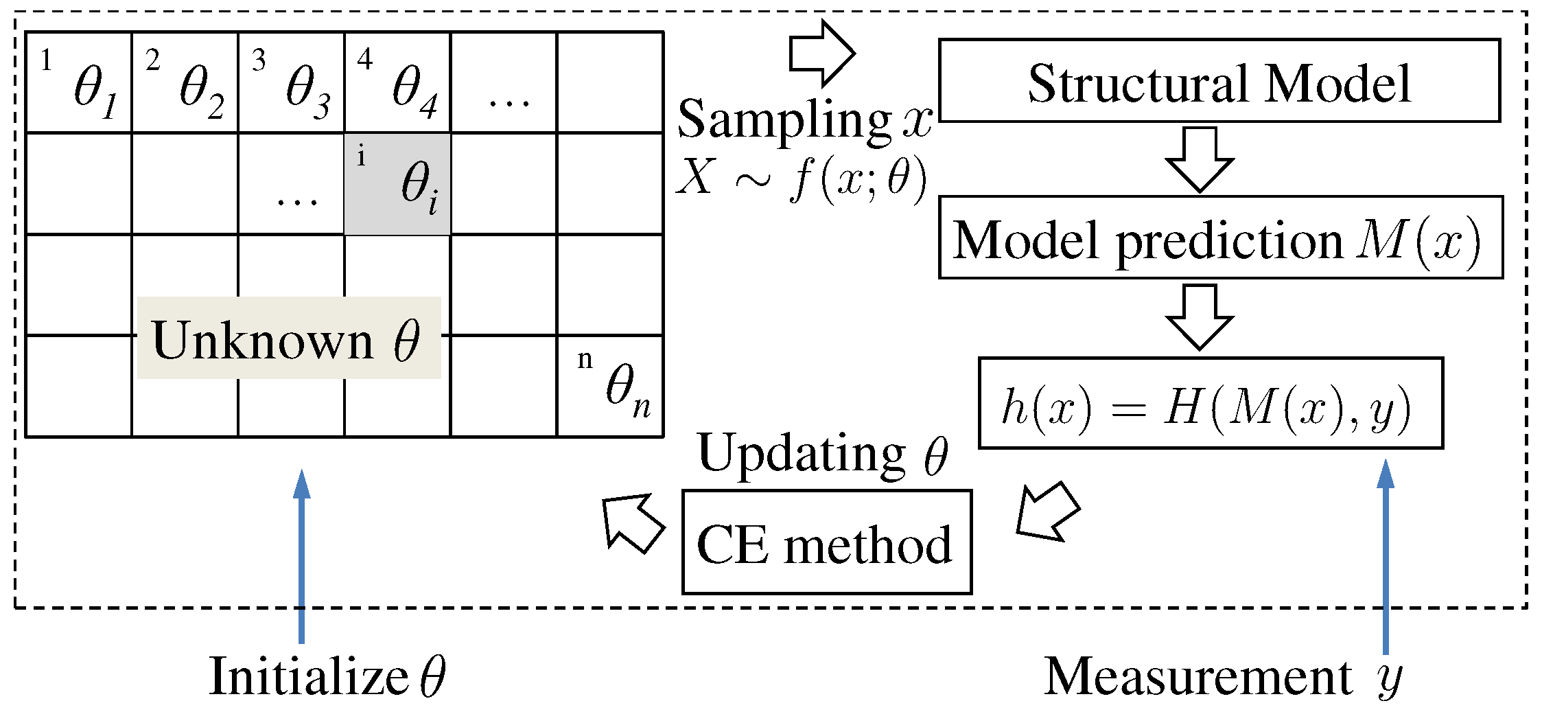
3. Formulation of Structural Component Damage Identification Using Cross-Entropy Optimizations

The starting point of structural damage identification using the cross-entropy optimization method is to formulate the problem as an optimization problem. Using vibration data, this can readily be made by comparing the actual vibration responses, such as frequencies and mode shapes, with its corresponding structural model predictions. A convenient model is a finite element (FE) model of the structure, where its components can be explicitly included. A damaged component can be represented in many ways such as reduction of the corresponding element stiffness or inertia in the representative FE model. Minimization of the difference between actual vibration responses and FE model predictions can be achieved when the actual structure and its FE model are well coupled.

In this study, the status of jth component in a representative FE model is modeled using a stiffness multiplier $x_j\in (0,1]$. For example, $x_j=1$ is the undamaged state of the component, and $x_j=0.5$ represents the stiffness of the component being reduced to 50% of its nominal value. Given a n-DOF (degree of freedom) FE model, the state of the entire system can be characterized using the vector of $\mathbf{x}=(x_1,x_2,...,x_n)$. The stiffness multipliers $x_1,x_2,...,x_n$ are assumed to be independent random variables since the damage states of components are independent. Many forms of distributions can be used to generate a random instance of $\mathbf{x}$ in the range of $(0,1]$. For simplicity, a truncated normal distribution in the range of $(0,1]$ with a constant standard deviation of $\sigma =0.05$ is used. In this setting, the distribution has one location parameter vector $\mathit{\theta }=({\theta }_1,{\theta }_2,...,{\theta }_n)$. For simplicity, the subscript j is omitted. The PDF of a truncated normal distribution in the range of $(a,b]$ is

$$f(x;\theta )=\varphi \left(\frac{x-\theta }{\sigma }\right)·Z^{-1},$$

(14)

where $\varphi (·)$ and $\mathsf{\Phi }(·)$ are PDF and cumulative distribution function (CDF) of a standard normal distribution, respectively, and $Z=\mathsf{\Phi }\left(\frac{b-\theta }{\sigma }\right)-\mathsf{\Phi }\left(\frac{a-\theta }{\sigma }\right)$ is the normalizing constant. The derivative of logarithm of the truncated PDF with respect to ${\theta }_i$ reads

$$\begin{array}{cc}\hfill \frac{\partial lnf(x;\theta )}{\partial \theta }& =\frac{\partial \left[-0.5·ln\left(2\pi \right)-ln\sigma -\frac{{\left(x-\theta \right)}^2}{2{\sigma }^2}\right]}{\partial \theta }-\left[\frac{\partial \mathsf{\Phi }\left(\frac{b-\theta }{\sigma }\right)}{\partial \theta }-\frac{\partial \mathsf{\Phi }\left(\frac{a-\theta }{\sigma }\right)}{\partial \theta }\right]·Z^{-1}\hfill \\ & =\frac{x-\theta }{{\sigma }^2}+\frac{1}{\sigma }\left[\varphi \left(\frac{b-\theta }{\sigma }\right)-\varphi \left(\frac{a-\theta }{\sigma }\right)\right]·Z^{-1}.\hfill \end{array}$$

(15)

Substitute Equation (15) into Equation (13) and obtain the updated θ for iterations as

$$\tilde{\theta }=\frac{{\sum }_{i=1}^N\mathbf{1}\left[h\left(X^{\left(i\right)}\right)\le \gamma \right]·X^{\left(i\right)}}{{\sum }_{i=1}^N\mathbf{1}\left[h\left(X^{\left(i\right)}\right)\le \gamma \right]}+\sigma ·\left[\varphi \left(\frac{b-\theta }{\sigma }\right)-\varphi \left(\frac{a-\theta }{\sigma }\right)\right]·Z^{-1}.$$

(16)

Equation (16) adjusts the usual estimator of an untruncated normal PDF by a constant term $c=\sigma ·\left[\varphi \left(\frac{b-\theta }{\sigma }\right)-\varphi \left(\frac{a-\theta }{\sigma }\right)\right]·Z^{-1}$. Under the condition that the mean value is away from the bounds and the standard deviation is small, using the untruncated estimator (the first term of the right-hand side of Equation (16)) can yield relative accurate results. For example, the relative error (RE) for θ estimation giving $a=0$, $b=1$, and $\sigma =0.05$ is shown in Figure 1. It can be seen that, when the stiffness multiplier is smaller than 0.95, the untruncated estimator yields an RE of about 0.1.

Without prior knowledge of the damage state of the structure, an initial value of ${\theta }_j=0.5$ ($j=1,\cdots ,n$) can be assigned. The assignment implies that each of the components of interest is multiplied by a normal random variable with a mean value of 0.5 and a standard deviation of 0.05. When an instance of the FE model is generated using a set of random values of $X_j$ drawn from its PDF, the calculated vibration characteristics such as natural frequencies and mode shapes are compared with the actual vibration characteristics extracted from the measurement data. When a random instance of the FE model minimizes the difference, the random instance is considered to be a close representation of the actual structure, and the values of ${\theta }_j$ are considered the actual stiffness multipliers. As a result, the damage identification problem is recast to an equivalent probabilistic optimization problem, which can be solved using the cross-entropy optimization algorithm shown in Algorithm 2. The basic procedure is as follows: generate a set of random instances of the FE models based on the current distribution parameter ${\theta }_j$; compare the difference between each of the random instance and the actual structure (e.g., using first several major frequencies); rank the difference and use samples that perform well to estimate new ${\theta }_j$ for the next iteration. The iteration stops when some criteria are met. The overall procedure is illustrated in Figure 2, where $M\left(x\right)$ denotes the prediction for the measured vibration response y and $X_j$ is the random realization for the stiffness multiplier of jth component. The algorithmic description of the proposed probabilistic damage identification method is summarized in Algorithm 3.

To perform the computation, N, M, $h\left(x\right)$, and $M\left(x\right)$ should be specified. The algorithm updates θ and ${\gamma }_t$ until θ is converged. At convergence, the first five ranking samples of $X_j$ is averaged as the final estimate for the stiffness multiplier of the jth component. A shear building damage identification problem with FE data is presented next.

Algorithm 3 Probabilistic Identification of Structural Damage

Set up a structural model $M\left(x\right)$ for response prediction, e.g., an FE model.  Define a performance function $h\left(x\right)$, e.g., $h\left(x\right)=\sum \left|M\right(x)-y|$, where y is measured response.  $t\leftarrow 0$.  Initialize ${\theta }_t$ and ${\gamma }_t$, e.g., ${\theta }_t=(0.5,\cdots ,0.5)$ and ${\gamma }_t=+\infty$.  repeat   (1) Draw N random variables $x^{\left(1\right)},\cdots ,x^{\left(N\right)}$ from $f(x;{\theta }_t)$.   (2) Calculate $h_i=h(x^{\left(i\right)})$ for all $i=1,\cdots ,N$ and sort $h_i$ from smallest to largest.   (3) ${\gamma }_t\leftarrow h_M$, where $1\le M\le N$.   (4) Calculate ${\theta }_{t+1}$ using Equation (16).   (5) $t\leftarrow t+1$.  until θ is converged.  Draw samples $x^{\left(1\right)},\cdots ,x^{\left(N\right)}$ from $f(x;{\theta }_t)$. $x_{*}$ is estimated by $\frac{1}{N}{\sum }_{i=1}^N{x}^{\left(i\right)}$.

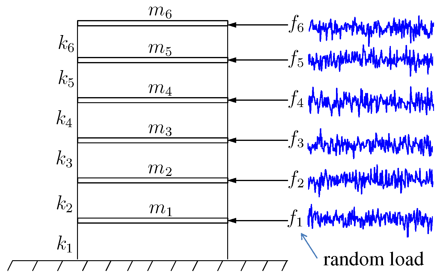
4. Application Example

A six-story shear building is used to illustrate the overall methodology and algorithms. The shear building is shown in Figure 3. The shear stiffness and mass for each floors are $\mathbf{k}=(k_1,\cdots ,k_6)$ and $\mathbf{m}=(m_1,\cdots ,m_6)$, respectively, from bottom to top. At each floor, random excitation forces $\mathbf{f}=(f_1,\cdots ,f_6)$ are applied to represent stochastic ambient loads. The global stiffness matrix and mass matrix are shown in Equations (17) and (18), respectively. To simulate actual measurements, acceleration responses of all floors are calculated by solving the equation of motions of the FE model. Noise terms are added to the deterministic calculation to represent the actual measurement uncertainty. Noise terms are characterized using Gauss pulse signal with a magnitude equal to a specified percentage of the maximum root mean square (RMS) of the deterministic calculation. Random excitation forces are generated using Gaussian white noise processes. Modal damping is used in this example to represent the actual damping effect. Four different combinations of damage location, measurement location, noise level, and damage severity are generated using the Latin hypercube sampling method to randomize the effect of those influencing factors:

$$\left[\mathbf{k}\right]=\left[\begin{array}{cccc}{k}_1+k_2& -k_2& \cdots & 0\\ -k_2& k_2+k_3& -k_3& 0\\ 0& -k_3& \cdots & \cdots \\ 0& 0& \cdots & k_6\end{array}\right],$$

(17)

$$\left[\mathbf{m}\right]=\left[\begin{array}{cccc}{m}_1& 0& \cdots & 0\\ 0& m_2& 0\cdots \\ 0& 0& \cdots & \cdots \\ 0& 0& \cdots & m_6\end{array}\right].$$

(18)

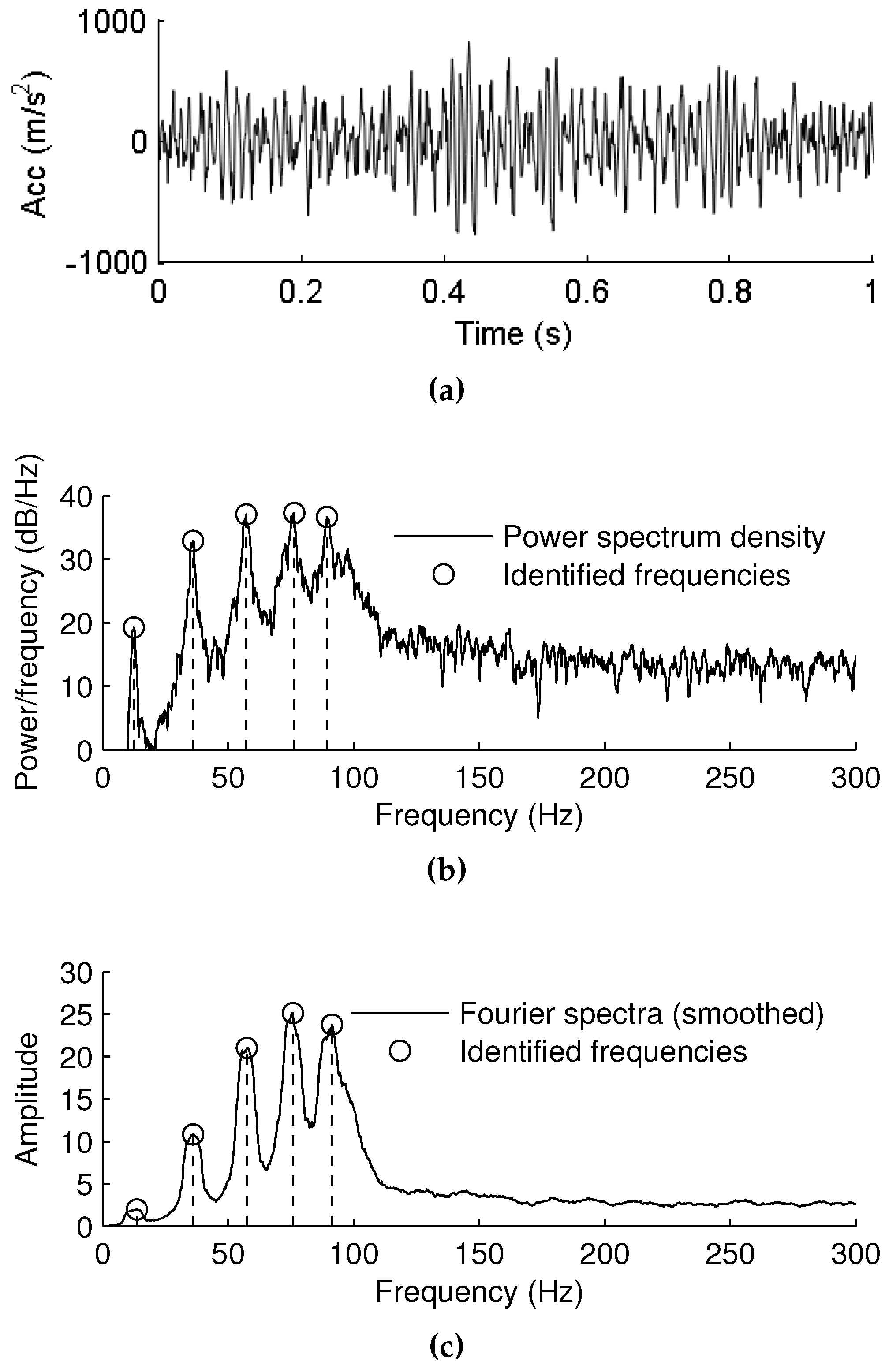
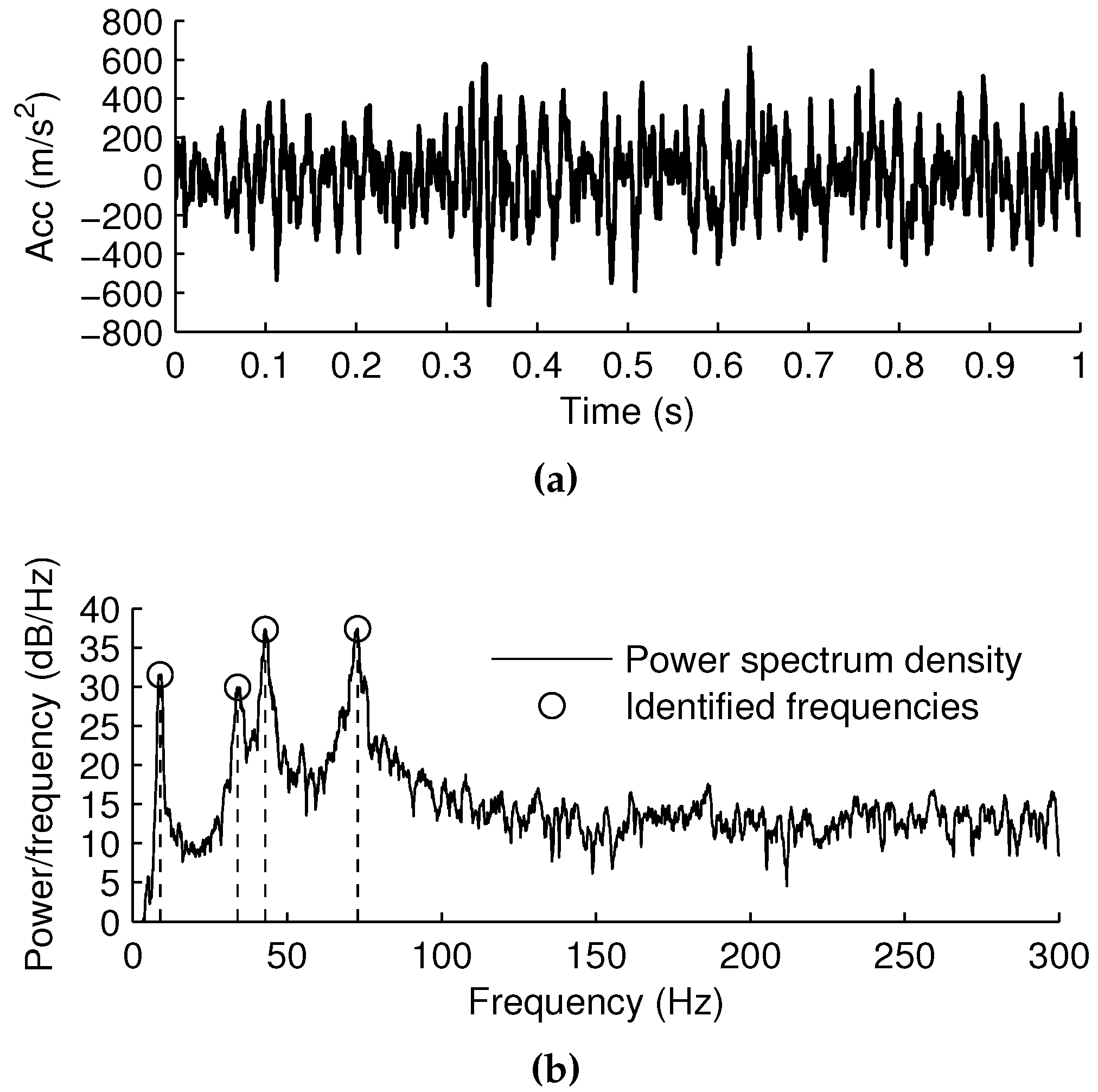
4.1. Measurement of Vibration Data and Extraction of Frequency Components

Acceleration responses are calculated by solving equations of motion of the shear building using the mode superposition method with a step size of $\mathrm{d}t$ = 0.001 s (i.e., the sampling frequency of the measurement is $1/\mathrm{d}t=1000$ Hz). For illustration purposes, shear stiffness of $\mathbf{k}=(k_1,\cdots ,k_6)=(100,100,100,100,100,100)\mathrm{GPa}$, the mass of $\mathbf{m}=(m_1,\cdots ,m_6)=(1,1,1,1,1,1)\times {10}^6\mathrm{kg}$, and a modal damping ratio of 0.02 are used. Responses of a duration of 5 s are calculated and responses of 0–1 s (normal state responses) measured at the first floor are shown in Figure 4a. The corresponding power spectra density and Fourier spectra are shown in Figure 4b,c, respectively. The identification of frequency components can be made using peak-picking methods. For this measurement data set, the identified frequency components are $(12.329,36.011,57.129,76.294,89.355)$.

4.2. Performance Function

The performance function $h\left(x\right)$ for ranking simulation samples can be established as follows. Given x as a random realization of the stiffness multiplier vector, the natural frequency of model $M\left(x\right)$ is calculated as

$$M\left(x\right)=\sqrt{\mathtt{eig}({\left[\mathbf{m}\right]}^{-1}\left[\mathbf{k}\right])}/\left(2\pi \right),$$

(19)

where $\mathtt{eig}(·)$ computes the eigenvalues. Denote the extracted v frequency components from measurement data as $f_{\mathrm{ext}}$. Simple performance measures, such as the sum of the squared error defined as $h\left(x\right)={\sum }_{i=1}^v{[M\left(x\right)-f_{\mathrm{ext}}]}^2$ and the sum of the absolute error defined as $h\left(x\right)={\sum }_{i=1}^v|M\left(x\right)-f_{\mathrm{ext}}|$, may not be suitable for realistic problems because weights of individual frequencies are not considered. Since the system is subject to random excitation forces, extracted frequency components will vary slightly. Therefore, frequency components can be modeled as a multivariate normal variable, and the the mean vector and covariance matrix can be statistically identified from multiple and independent measurement datasets. It can increase the robustness of the performance measure and weight each frequency components appropriately. A general formulation of the performance function $h\left(x\right)$ is proposed as the log-likelihood of the multivariate normal PDF

$$h\left(x\right)\propto (M\left(x\right)-{\mu }_f)·{\mathsf{\Sigma }}_f^{-1}·{(M\left(x\right)-{\mu }_f)}^T,$$

(20)

where ${\mu }_f$ and ${\mathsf{\Sigma }}_f$ are the mean vector and covariance matrix of the extracted frequency components, and ${[·]}^T$ is the transpose operator. In realistic applications, ${\mu }_f$ and ${\mathsf{\Sigma }}_f$ can be estimated from multiple successive measurements. Equation (20) can easily be transformed to a multivariate normal PDF as ${\left(2\pi \right)}^{-v/2}{\left|{\mathsf{\Sigma }}_f\right|}^{-1/2}exp[-\frac{1}{2}h\left(x\right)]$.

4.3. Damage Identification

Four cases are studied to investigate the effectiveness of the method. Factors considered are damage location (floor $1,\cdots ,6$), measurement location (floor $1,\cdots ,6$), measurement noise ($5\%,10\%,20\%$), and damage severity represented by the stiffness multiplier ($0.925,0.9,0.85,0.8$). Latin hypercube sampling [44] is used to generate four cases as shown in

Table 1. Damage cases generated using Latin hypercube sampling.

Case	Damage Component	Measurement Location	Measurement Noise	Stiffness Reduced by
1	floor 3	floor 3	10%	0.9
2	floor 4	floor 1	5%	0.8
3	floor 6	floor 4	20%	0.85
4	floor 1	floor 6	10%	0.925

.

4.3.1. Case 1

Measurement data of system acceleration are generated using the procedure and setting described in Section 4.1. The only difference is that the shear stiffness of floor 3 is $0.9\times k_3=90\mathrm{GPa}$, representing the damage. To obtain ${\mu }_f$ and ${\mathsf{\Sigma }}_f$, a total of 500 s of measurement data are generated, and the time series are divided into 100 pieces evenly. For each piece, the frequency components are extracted. ${\mu }_f$ and ${\mathsf{\Sigma }}_f$ are then estimated from 100 sets of extracted frequency components. For example, the first five seconds of response measurement data are shown in Figure 5a, and identified frequency components are shown in Figure 5b. The mean vector ${\mu }_{f:\mathrm{case}1}$ and covariance matrix ${\mathsf{\Sigma }}_{f:\mathrm{case}1}$ of the identified frequency components are estimated as

$${\mu }_{f:\mathrm{case}1}=(12.073,35.73,56.321,75.261)$$

(21)

and

$${\mathsf{\Sigma }}_{f:\mathrm{case}1}=\left[\begin{array}{cccc}0.057648& 0.0063217& -0.0090611& -0.011078\\ 0.0063217& 0.12809& 0.016768& -0.0037328\\ -0.0090611& 0.016768& 0.23384& -0.013173\\ -0.011078& -0.0037328& -0.013173& 0.32825\end{array}\right],$$

(22)

respectively.

The vector θ is initialized as ${\theta }_{1,\cdots ,6}=(0.5,0.5,0.5,0.5,0.5,0.5)$, and $N=1000$ and $M=30$ are used. Using Algorithm 3, iterative results are shown in

Table 2. Convergence of damage state probability distribution parameter θ of Case 1.

t	${\mathit{\theta }}_1$	${\mathit{\theta }}_2$	${\mathit{\theta }}_3$	${\mathit{\theta }}_4$	${\mathit{\theta }}_5$	${\mathit{\theta }}_6$	${\mathit{\gamma }}_{\mathit{t}}$
0	0.5	0.5	0.5	0.5	0.5	0.5	+∞
1	0.72	0.57	0.67	0.70	0.65	0.74	987.818
2	0.91	0.75	0.82	0.88	0.87	0.93	201.615
3	0.97	0.93	0.95	0.98	0.95	0.97	16.973
4	0.99	0.99	0.96	1.00	0.99	1.00	1.738
*	1.00	1.00	0.92	1.00	1.00	1.00	0.180

. The converged result of ${\theta }_{1,\cdots ,6}=(1.00,1.00,0.92,1.00,1.00,1.00)$ indicates that floor 3 is damaged, i.e., ${\theta }_3=0.92$. The result is obtained with four iterations in about 0.16 seconds using the $\mathrm{MATLAB}$ software package.

4.3.2. Case 2

In this case, the first five frequency components can be identified from the acceleration measurement data taken from floor 1. Measurement data and the corresponding power spectrum density plots are not presented hereafter. Using the same procedure and parameters as that of Case 1, ${\mu }_{f:\mathrm{case}2}$ and ${\mathsf{\Sigma }}_{f:\mathrm{case}2}$ are obtained as

$${\mu }_{f:\mathrm{case}2}=(12.002,34.843,56.816,73.107,88.842)$$

(23)

and

$${\mathsf{\Sigma }}_{f:\mathrm{case}2}=\left[\begin{array}{ccccc}0.051742& 0.003197& 0.020759& 0.0011319& -0.0089226\\ 0.003197& 0.13855& 0.0046781& -0.039175& 0.010089\\ 0.020759& 0.0046781& 0.22918& 0.018038& 0.019904\\ 0.0011319& -0.039175& 0.018038& 0.45453& 0.0088338\\ -0.0089226& 0.010089& 0.019904& 0.0088338& 0.50312\end{array}\right],$$

(24)

respectively. Intermediate and converged results for θ are shown in

Table 3. Convergence of damage state probability distribution parameter θ of Case 2.

t	${\mathit{\theta }}_1$	${\mathit{\theta }}_2$	${\mathit{\theta }}_3$	${\mathit{\theta }}_4$	${\mathit{\theta }}_5$	${\mathit{\theta }}_6$	${\mathit{\gamma }}_{\mathit{t}}$
0	0.5	0.5	0.5	0.5	0.5	0.5	+∞
1	0.72	0.61	0.68	0.68	0.67	0.75	965.583
2	0.89	0.79	0.85	0.85	0.87	0.94	177.565
3	0.97	0.96	0.97	0.95	0.98	0.97	12.256
4	0.96	0.98	0.98	0.87	0.99	0.99	3.803
*	0.99	1.00	0.99	0.81	0.99	1.00	0.751

. The converged results of ${\theta }_{1,\cdots ,6}=(0.99,1.00,0.99,0.81,0.99,1.00)$ indicates that floor 4 is damaged with an estimated stiffness reduced to 81% of its nominal value. The result is obtained with four iterations in about 0.15 seconds using ${\mathrm{MATLAB}}^{\circledR }$.

4.3.3. Case 3

The same procedure is applied for estimation of ${\mu }_{f:\mathrm{case}3}$ and ${\mathsf{\Sigma }}_{f:\mathrm{case}3}$ and detailed results are presented below. The converged result of θ is presented in

Table 4. Convergence of damage state probability distribution parameter θ of Case 3.

t	${\mathit{\theta }}_1$	${\mathit{\theta }}_2$	${\mathit{\theta }}_3$	${\mathit{\theta }}_4$	${\mathit{\theta }}_5$	${\mathit{\theta }}_6$	${\mathit{\gamma }}_{\mathit{t}}$
0	0.5	0.5	0.5	0.5	0.5	0.5	+∞
1	0.71	0.63	0.69	0.67	0.65	0.74	1068.041
2	0.90	0.81	0.86	0.86	0.85	0.93	194.705
3	0.97	0.96	0.96	0.96	0.97	0.97	12.073
4	0.98	0.99	0.97	0.96	0.99	0.93	3.316
*	0.98	1.00	1.00	0.99	1.00	0.86	0.399

and floor 6 is identified as a damaged component

$${\mu }_{f:\mathrm{case}3}=(12.213,35.339,55.901,73.962,88.293),$$

(25)

$${\mathsf{\Sigma }}_{f:\mathrm{case}3}=\left[\begin{array}{ccccc}0.043198& -0.0015503& -0.035251& -0.01299& -0.011831\\ -0.0015503& 0.10389& 0.0026732& -0.0063684& -0.033087\\ -0.035251& 0.0026732& 0.21991& 0.010199& 0.0123\\ -0.01299& -0.0063684& 0.010199& 0.35465& 0.022304\\ -0.011831& -0.033087& 0.0123& 0.022304& 0.52409\end{array}\right].$$

(26)

4.3.4. Case 4

The estimation of ${\mu }_{f:\mathrm{case}4}$ and ${\mathsf{\Sigma }}_{f:\mathrm{case}4}$ follows the same procedure as the one used in previous cases. Detailed results are presented below. The converged result of θ shown in

Table 5. Convergence of damage state probability distribution parameter θ of Case 4.

t	${\mathit{\theta }}_1$	${\mathit{\theta }}_2$	${\mathit{\theta }}_3$	${\mathit{\theta }}_4$	${\mathit{\theta }}_5$	${\mathit{\theta }}_6$	${\mathit{\gamma }}_{\mathit{t}}$
0	0.5	0.5	0.5	0.5	0.5	0.5	+∞
1	0.72	0.61	0.68	0.68	0.67	0.75	1065.796
2	0.89	0.79	0.85	0.85	0.87	0.94	222.107
3	0.97	0.95	0.96	0.97	0.97	0.97	18.414
4	0.99	0.99	0.98	0.99	0.99	1.00	0.986
*	0.96	1.00	1.00	1.00	0.98	1.00	0.124

indicates that floor 1 is damaged:

$${\mu }_{f:\mathrm{case}4}=(12.003,35.359,56.819,75.04,88.752),$$

(27)

$${\mathsf{\Sigma }}_{f:\mathrm{case}4}=\left[\begin{array}{ccccc}0.056611& 0.0025919& 0.021196& -0.0013682& 0.0045185\\ 0.0025919& 0.1545& 0.011235& -0.026518& -0.019712\\ 0.021196& 0.011235& 0.24125& -0.014386& 0.008164\\ -0.0013682& -0.026518& -0.014386& 0.4786& 0.021467\\ 0.0045185& -0.019712& 0.008164& 0.021467& 0.48401\end{array}\right].$$

(28)

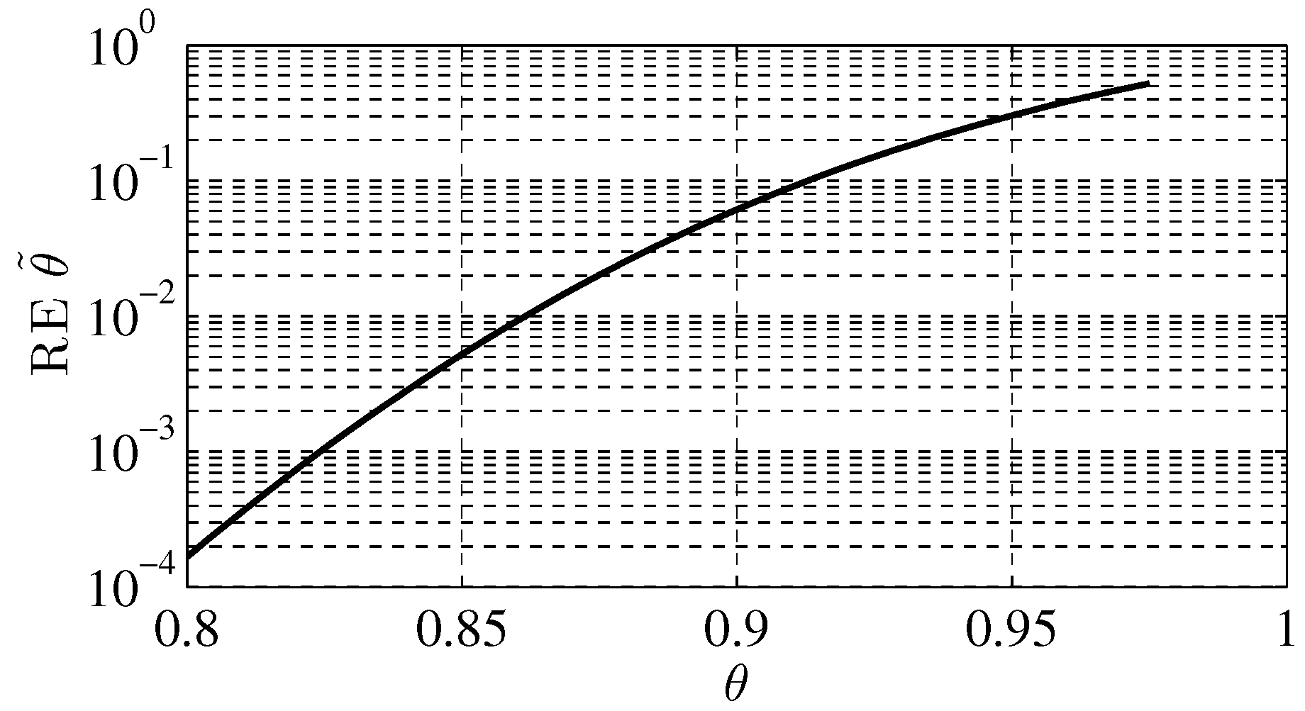
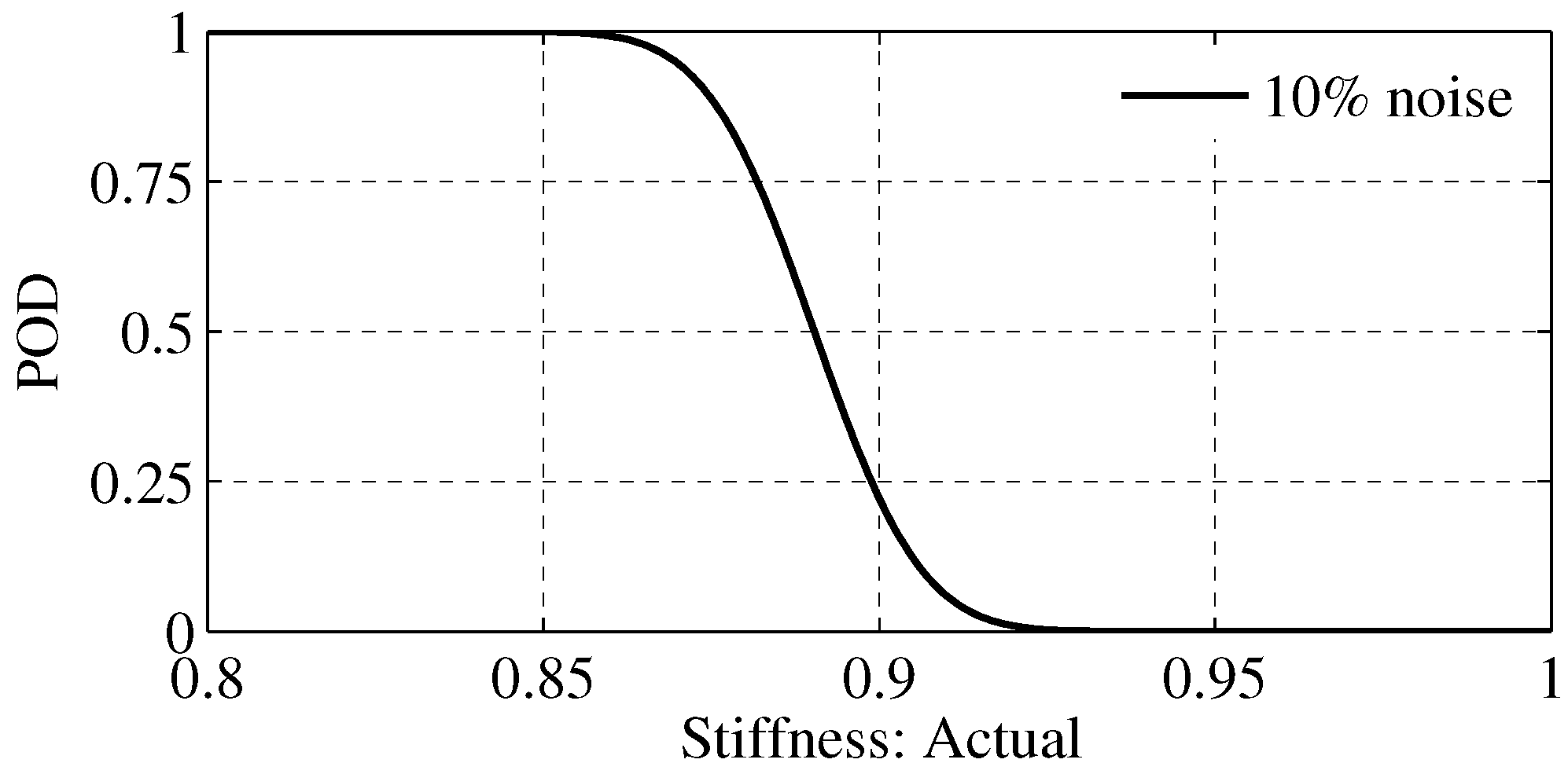
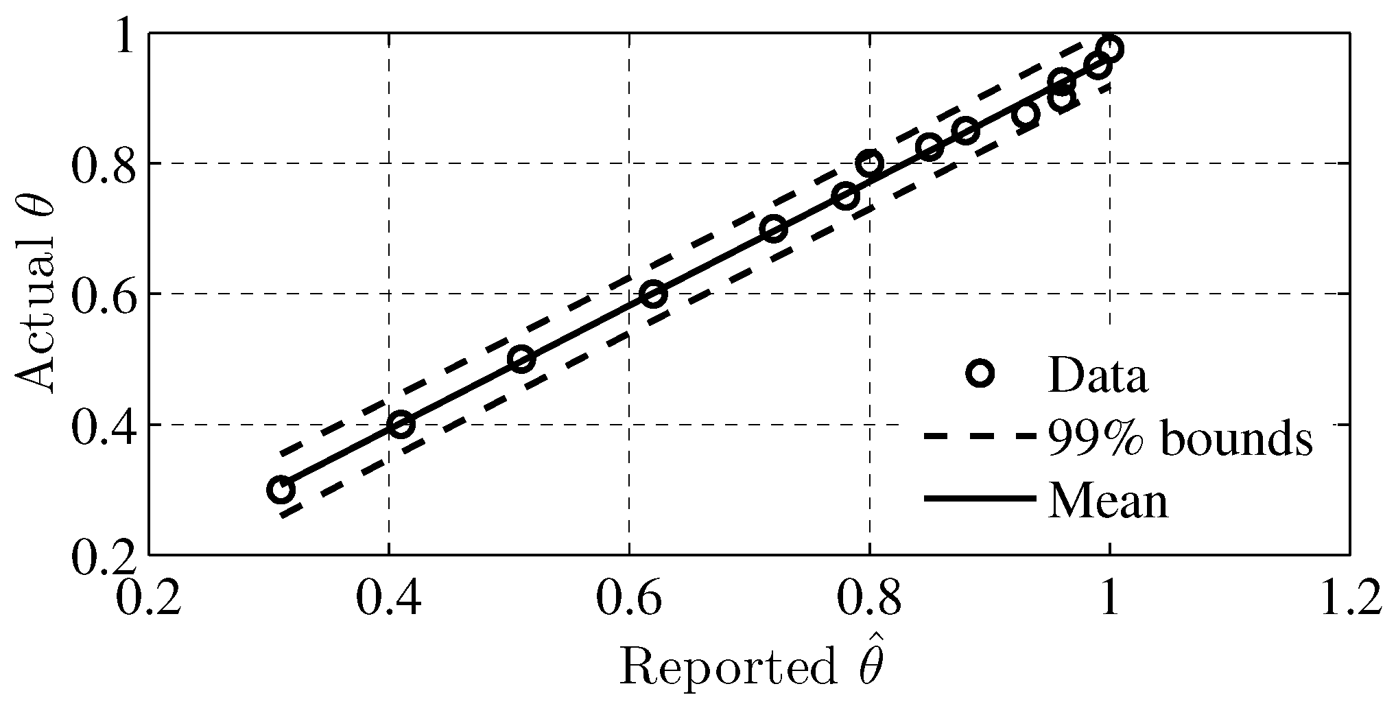
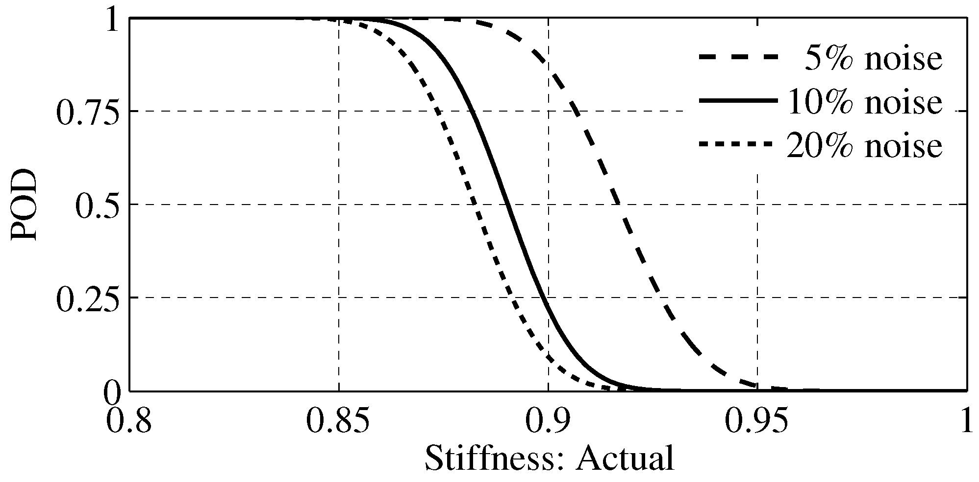
4.4. Probability of Detection

The probability of detection (POD) of the damage identification method can be quantified using classical linear models [10,20,45]. Denote the reported stiffness multiplier as $\widehat{\theta }$ and the actual stiffness multiplier as θ. The linear model for POD reads

$$\theta =\alpha +\beta \times \widehat{\theta }+ϵ,$$

(29)

where ϵ is a normal random variable with zero mean and standard deviation ${\sigma }_{ϵ}$, and α and β are fitting parameters. Note that when the actual stiffness multiplier is close to 1, the method cannot differentiate the slight damage from its healthy state since the damage only imposes a minimal influence to the change of its natural frequencies; therefore, the damage is regarded as identified if the reported stiffness multiplier $\widehat{\theta }$ is smaller than the detection threshold $\widehat{{\theta }_{\mathrm{th}}}$. The value of $\widehat{{\theta }_{\mathrm{th}}}$ is specified based on measurement uncertainty and limits of the detection method. The probability of detection can be expressed as $\mathrm{POD}\left(\theta \right)=\mathrm{Pr}(\widehat{\theta }<\widehat{{\theta }_{\mathrm{th}}})$, where $\mathrm{Pr}(·)$ represents the probability of an event $(·)$. Using Equation (29) the POD writes

$$\mathrm{POD}\left(\theta \right)=\mathsf{\Phi }\left(\frac{\alpha +\beta \times \widehat{{\theta }_{\mathrm{th}}}-a}{{\sigma }_{ϵ}}\right).$$

(30)

A set of numerical experiments are performed, and the configuration of Case 4 for measurement location, damage location, and noise level is used. Multiple values of θ in the range of [0.3,0.975] are used to represent different damage severities. For each θ, a numerical simulation is conducted to acquire the measurement data. A set of ($\widehat{\theta }$, θ) values are obtained and shown in

Table 6. Actual stiffness and reported stiffness of the proposed method. The configuration of Case 4 is used for measurement location, noise level, and damage location.

Actual	0.3	0.4	0.5	0.6	0.7	0.75	0.8	0.825	0.85	0.875	0.9	0.925	0.95	0.975
Reported	0.31	0.41	0.51	0.62	0.72	0.78	0.8	0.85	0.88	0.93	0.96	0.96	0.99	1

. It is noticed that when the actual stiffness multiplier is larger than 0.95, it is difficult for the method to differentiate the slight change of the stiffness from its healthy state; therefore, the threshold $\widehat{{\theta }_{\mathrm{th}}}$ is conservatively assumed to be 0.925. The linear model fitting parameters α and β are 0.0132 and 0.9482, respectively. The standard deviation of the normal random variable ϵ is estimated as ${\sigma }_{ϵ}=0.0126$. The data and model predictions are presented in Figure 6. Given α, β, ${\sigma }_{ϵ}$, and $\widehat{{\theta }_{\mathrm{th}}}$, the POD curve of the damage identification method is calculated and is shown in Figure 7. It can be seen that the method can reliably identify the damage and estimate the stiffness multiplier when the actual stiffness multiplier is 0.85 or smaller.

To further investigate the influence of the noise, numerical experiments under noise levels of 5% and 20% are conducted. All other procedures are identical to the above 10% noise level case. POD curves associated with 5% and 20% noise levels are calculated and presented in Figure 8. In the figure, 90% POD identification capabilities for stiffness multipliers are 0.897, 0.874, and 0.866 under 5%, 10%, and 20% noise levels, respectively. The identification capabilities increase to 0.917, 0.890, 0.882 at POD = 50%.

Results of the numerical example demonstrate that the proposed method can reliably identify the damaged component and estimate the stiffness multiplier within a few iterations. Since the performance function is a multivariate normal distribution with parameters obtained from measurement data of the structure being considered, the influence from measurement noise can be effectively incorporated into the performance function using the covariance matrix of the normal distribution. The measurement location has no significant effect on the final result. It should be noted that the method can also be used for a more general structure given that the damage and normal state of a component can be modeled using a random variable, and modal frequencies can be reliably extracted from the measurement data.

5. Conclusions

This study developed a probabilistic damage identification method for shear structures using cross-entropy optimization. The method uses the modal frequencies extracted from acquired vibration data such as accelerations under random loading in conjunction with a representative finite element model. Multiple measurement data sets are used to extract the modal frequencies independently. A multivariate normal distribution is built and its mean vector and covariance matrix are used to construct the performance function. The damage is characterized by a stiffness multiplier of each component of the shear structure. The multiplier is valued in the range of (0,1], where 1 and 0 indicate undamaged and completely damaged, respectively. The multiplier is modeled using a truncated normal variable with an initial mean value of 0.5 and a constant standard deviation. By randomly generating a set of multipliers, the modal frequencies are computed and compared with the actual modal frequencies extracted from the measurement data. The cross-entropy optimization algorithm iteratively updates the mean value of the distribution of each multipliers until convergence. At convergence, the first few samples is averaged to obtain the final estimation of the stiffness multiplier. The overall method is demonstrated using a six-story shear structure with four damage cases generated by Latin hypercube sampling on damage location, measurement location, measurement noise level, and damage severity. The sensitivity of the method is further investigated using POD models under different noise levels. Numerical results suggest that the proposed method provides a viable solution for shear structure damage identification and quantification. The detection reliability reduces as the noise level increases. For a moderate 5% noise level, the method can identify a reduction of 10% of its nominal stiffness with a probability of 90%. When the probability of detection is 50%, the method can identify a reduction of 8% of its nominal stiffness.

The potential limitations of the method are: (1) the accuracy and uncertainty in modal frequency extraction, and (2) the inevitable mismatch from the representative FE model and the real structure. For practical applications, the latter limitation is an inherent disadvantage for modal frequency methods with representative FE models. Model updating techniques can be greatly helpful until a certain level of representation accuracy. The damage identification method can fail or become less effective if the FE model cannot represent the real structure accurately. It should be noted that the simulation of the damage through the stiffness multiplier is a simplification of the actual complex damage variability. The damage identification method using cross-entropy optimization for other structures (e.g., 3D solid) is planned for future study. In addition, using other modal features such as mode shapes to build the performance measure will be investigated later.

References

1. Doebling, S.; Farrar, C.; Prime, M.; Shevitz, D. Damage Identification and Health Monitoring of Structural and Mechanical Systems from Changes in Their Vibration Characteristics: A Literature Review; Technical Report LA–13070-MS; Los Alamos National Lab: Los Alamos, NM, USA, May 1996. [Google Scholar]
2. Fan, W.; Qiao, P. Vibration-based damage identification methods: A review and comparative study. Struct. Health Monit. 2011, 10, 83–111. [Google Scholar] [CrossRef]
3. Dessi, D.; Camerlengo, G. Damage identification techniques via modal curvature analysis: Overview and comparison. Mech. Syst. Signal Process. 2015, 52, 181–205. [Google Scholar] [CrossRef]
4. Jardine, A.; Lin, D.; Banjevic, D. A review on machinery diagnostics and prognostics implementing condition-based maintenance. Mech. Syst. Signal Process. 2006, 20, 1483–1510. [Google Scholar] [CrossRef]
5. Li, H.N.; Li, D.S.; Ren, L.; Yi, T.H.; Jia, Z.G.; LI, K.P. Structural health monitoring of innovative civil engineering structures in Mainland China. Struct. Monit. Maint. 2016, 3, 1–32. [Google Scholar] [CrossRef]
6. Rytter, A. Vibrational Based Inspection of Civil Engineering Structures. Ph.D. Thesis, Aalborg University, Aalborg, Denmark, April 1993. [Google Scholar]
7. Blitz, J.; Simpson, G. Ultrasonic Methods of Non-Destructive Testing; Champman & Hall: London, UK, 1996; Volume 2. [Google Scholar]
8. Drinkwater, B.; Wilcox, P. Ultrasonic arrays for non-destructive evaluation: A review. NDT & E Int. 2006, 39, 525–541. [Google Scholar]
9. Guan, X.; Zhang, J.; Rasselkorde, E.M.; Abbasi, W.A.; Zhou, S.K. Material damage diagnosis and characterization for turbine rotors using three-dimensional adaptive ultrasonic NDE data reconstruction techniques. Ultrasonics 2014, 54, 516–525. [Google Scholar] [CrossRef] [PubMed]
10. Guan, X.; Zhang, J.; Zhou, S.K.; Rasselkorde, E.M.; Abbasi, W. Probabilistic modeling and sizing of embedded flaws in ultrasonic non-destructive inspections for fatigue damage prognostics and structural integrity assessment. NDT & E Int. 2014, 61, 1–9. [Google Scholar]
11. Guan, X.; Zhang, J.; Zhou, S.K.; Rasselkorde, E.M.; Abbasi, W.A. Post-processing of phased-array ultrasonic inspection data with parallel computing for nondestructive evaluation. J. Nondestruct. Eval. 2014, 33, 342–351. [Google Scholar] [CrossRef]
12. Guan, X.; He, J.; Rasselkorde, E.M. A time-domain synthetic aperture ultrasound imaging method for material flaw quantification with validations on small-scale artificial and natural flaws. Ultrasonics 2015, 56, 487–496. [Google Scholar] [CrossRef] [PubMed]
13. Guan, X.; Rasselkorde, E.M.; Abbasi, W.A.; Zhou, S.K. Turbine fatigue reliability and life assessment using ultrasonic inspection: Data acquisition, interpretation, and probabilistic modeling. In Quality and Reliability Management and Its Applications; Springer: London, UK, 2016; pp. 415–434. [Google Scholar]
14. Bowler, J. Eddy-current interaction with an ideal crack. I. The forward problem. J. Appl. Phys. 1994, 75, 8128–8137. [Google Scholar] [CrossRef]
15. Takagi, T.; Huang, H.; Fukutomi, H.; Tani, J. Numerical evaluation of correlation between crack size and eddy current testing signal by a very fast simulator. IEEE Trans. Magn. 1998, 34, 2581–2584. [Google Scholar] [CrossRef]
16. Kessler, S.; Spearing, S.; Soutis, C. Damage detection in composite materials using Lamb wave methods. Smart Mater. Struct. 2002, 11, 269. [Google Scholar] [CrossRef]
17. Ostachowicz, W.; Kudela, P.; Malinowski, P.; Wandowski, T. Damage localisation in plate-like structures based on PZT sensors. Mech. Syst. Signal Process. 2009, 23, 1805–1829. [Google Scholar] [CrossRef]
18. He, J.; Guan, X.; Peng, T.; Liu, Y.; Saxena, A.; Celaya, J.; Goebel, K. A multi-feature integration method for fatigue crack detection and crack length estimation in riveted lap joints using Lamb waves. Smart Mater. Struct. 2013, 22, 105007. [Google Scholar] [CrossRef]
19. He, J.; Zhou, Y.; Guan, X.; Zhang, W.; Wang, Y.; Zhang, W. An integrated health monitoring method for structural fatigue life evaluation using limited sensor data. Materials 2016, 9, 894. [Google Scholar] [CrossRef]
20. Yang, J.; He, J.; Guan, X.; Wang, D.; Chen, H.; Zhang, W.; Liu, Y. A probabilistic crack size quantification method using in-situ Lamb wave test and Bayesian updating. Mech. Syst. Signal Process. 2016, 78, 118–133. [Google Scholar] [CrossRef]
21. He, J.; Zhou, Y.; Guan, X.; Zhang, W.; Zhang, W.; Liu, Y. Time domain strain/stress reconstruction based on empirical mode decomposition: numerical study and experimental validation. Sensors 2016, 16, 1290. [Google Scholar] [CrossRef] [PubMed]
22. Farrar, C.; Doebling, S.; Nix, D. Vibration-based structural damage identification. Phil. Trans. R. Soc. Lond. A 2001, 359, 131–149. [Google Scholar] [CrossRef]
23. Yan, Y.; Cheng, L.; Wu, Z.; Yam, L. Development in vibration-based structural damage detection technique. Mech. Syst. Signal Process. 2007, 21, 2198–2211. [Google Scholar] [CrossRef]
24. Salawu, O. Detection of structural damage through changes in frequency: A review. Eng. Struct. 1997, 19, 718–723. [Google Scholar] [CrossRef]
25. Cawley, P.; Adams, R. A vibration technique for non-destructive testing of fibre composite structures. J. Compos. Mater. 1979, 13, 161. [Google Scholar] [CrossRef]
26. Friswell, M.; Penny, J.; Wilson, D. Using vibration data and statistical measures to locate damage in structures. Int. J. Anal. Exp. Modal Anal. 1994, 9, 239–254. [Google Scholar]
27. Fritzen, C.; Jennewein, D.; Kiefer, T. Damage detection based on model updating methods. Mech. Syst. Signal Process. 1998, 12, 163–186. [Google Scholar] [CrossRef]
28. Bayissa, W.; Haritos, N.; Thelandersson, S. Vibration-based structural damage identification using wavelet transform. Mech. Syst. Signal Process. 2008, 22, 1194–1215. [Google Scholar] [CrossRef]
29. Deraemaeker, A.; Reynders, E.; De Roeck, G.; Kullaa, J. Vibration-based structural health monitoring using output-only measurements under changing environment. Mech. Syst. Signal Process. 2008, 22, 34–56. [Google Scholar] [CrossRef]
30. Fugate, M.; Sohn, H.; Farrar, C. Vibration-based damage detection using statistical process control. Mech. Syst. Signal Process. 2001, 15, 707–721. [Google Scholar] [CrossRef]
31. Doebling, S.W.; Farrar, C.R.; Prime, M.B. A summary review of vibration-based damage identification methods. Shock Vib. Dig. 1998, 30, 91–105. [Google Scholar] [CrossRef]
32. Li, H.; Bao, Y.; Ou, J. Structural damage identification based on integration of information fusion and shannon entropy. Mech. Syst. Signal Process. 2008, 22, 1427–1440. [Google Scholar] [CrossRef]
33. Papadimitriou, C.; Beck, J.; Katafygiotis, L. Updating robust reliability using structural test data. Probabilist. Eng. Mech. 2001, 16, 103–113. [Google Scholar] [CrossRef]
34. Sohn, H.; Law, K.H. A Bayesian probabilistic approach for structure damage detection. Earthq. Eng. Struct. Dyn. 1997, 26, 1259–1281. [Google Scholar] [CrossRef]
35. Worden, K.; Farrar, C.R.; Haywood, J.; Todd, M. A review of nonlinear dynamics applications to structural health monitoring. Struct. Control Health Monit. 2008, 15, 540–567. [Google Scholar] [CrossRef]
36. Behmanesh, I.; Moaveni, B.; Lombaert, G.; Papadimitriou, C. Hierarchical Bayesian model updating for structural identification. Mech. Syst. Signal Process. 2015, 64, 360–376. [Google Scholar] [CrossRef]
37. Friswell, M.; Mottershead, J.E. Finite Element Model Updating in Structural Dynamics; Springer Science & Business Media: Dordrecht, The Netherlands, 1995; Volume 38. [Google Scholar]
38. Mottershead, J.; Friswell, M. Model updating in structural dynamics: A survey. J. Sound Vib. 1993, 167, 347–375. [Google Scholar] [CrossRef]
39. Yuen, K.V.; Beck, J.L.; Katafygiotis, L.S. Unified probabilistic approach for model updating and damage detection. J. Appl. Mech. 2006, 73, 555–564. [Google Scholar] [CrossRef]
40. Rubinstein, R. The cross-entropy method for combinatorial and continuous optimization. Methodol. Comput. Appl. Probab. 1999, 1, 127–190. [Google Scholar] [CrossRef]
41. Rubinstein, R.; Kroese, D. The Cross-Entropy Method: A Unified Approach to Combinatorial Optimization, Monte-Carlo Simulation, and Machine Learning; Springer: New York, NY, USA, 2004. [Google Scholar]
42. Kroese, D.P.; Porotsky, S.; Rubinstein, R.Y. The cross-entropy method for continuous multi-extremal optimization. Methodol. Comput. Appl. Probab. 2006, 8, 383–407. [Google Scholar] [CrossRef]
43. Kullback, S.; Leibler, R. On information and sufficiency. Ann. Math. Stat. 1951, 22, 79–86. [Google Scholar] [CrossRef]
44. Park, J. Optimal Latin-hypercube designs for computer experiments. J. Stat. Plan. Inference 1994, 39, 95–111. [Google Scholar] [CrossRef]
45. Guan, X.; He, J.; Rasselkorde, E.M.; Zhang, J.; Abbasi, W.A.; Zhou, S.K. Probabilistic fatigue life prediction and structural reliability evaluation of turbine rotors integrating an automated ultrasonic inspection system. J. Nondestruct. Eval. 2014, 33, 51–61. [Google Scholar] [CrossRef]
Figure 1. Relative error (RE) of updated theta calculated using untruncated normal estimator.
Entropy 19 00027 g001
Figure 2. Procedure of probabilistic damage identification. The performance function h ( x ) defines a measure to quantify the performance of a random realization of X.
Entropy 19 00027 g002
Figure 3. Diagram of the six-story shear building and external random excitation forces.
Entropy 19 00027 g003
Figure 4. Frequency components identified from acceleration measurement at floor 1. (a) Measurement data; (b) power spectra density; and (c) Fourier spectra.
Entropy 19 00027 g004
Figure 5. (a) measurement data of acceleration responses at floor 3 and (b) identified frequency components.
Entropy 19 00027 g005
Figure 6. Mean and bound predictions obtained by the linear model of Equation (29).
Entropy 19 00027 g006
Figure 7. POD curve of the damage identification method for case 4.
Entropy 19 00027 g007
Figure 8. POD curves under different levels of RMS noise components in measurement data. Other settings are identical to Case 4.
Entropy 19 00027 g008