Article

Exploitation of the Maximum Entropy Principle in Mathematical Modeling of Charge Transport in Semiconductors

by
Giovanni Mascali
1,*,† and
Vittorio Romano
2,†
1
Dipartimento di Matematica ed Informatica, Università della Calabria e INFN-Gruppo c. Cosenza, Rende 87036, Italy
2
Dipartimento di Matematica ed Informatica, Università di Catania, Catania 95125, Italy
*
Author to whom correspondence should be addressed.
These authors contributed equally to this work.
Entropy 2017, 19(1), 36; https://doi.org/10.3390/e19010036
Submission received: 7 November 2016 / Revised: 4 January 2017 / Accepted: 5 January 2017 / Published: 18 January 2017
(This article belongs to the Special Issue Maximum Entropy Principle and Semiconductors)

Abstract

:
In the last two decades, the Maximum Entropy Principle (MEP) has been successfully employed to construct macroscopic models able to describe the charge and heat transport in semiconductor devices. These models are obtained, starting from the Boltzmann transport equations, for the charge and the phonon distribution functions, by taking—as macroscopic variables—suitable moments of the distributions and exploiting MEP in order to close the evolution equations for the chosen moments. Important results have also been obtained for the description of charge transport in devices made both of elemental and compound semiconductors, in cases where charge confinement is present and the carrier flow is two- or one-dimensional.

1. Introduction

In the design of new generation electronic devices, the modern micro- and nanoelectronics industry has an increasing need for mathematical models to simulate devices before they are realized in the laboratory. In particular, the accurate modeling of energy transport in semiconductors is necessary in order to describe high-field phenomena, such as hot electron propagation, impact ionization and heat generation in the bulk material. Semiclassically, the most effective way to describe these phenomena makes use of the semiclassical Boltzmann Transport Equation (BTE) [1]. However, solving the BTE is a daunting computational task, both using an indirect stochastic approach by Monte Carlo methods and direct numerical schemes based on discontinuous Galerkin methods or finite differences [2]. This is the reason why, in many cases, it is desirable to have simpler macroscopical models, known as hydrodynamical-like models, which are highly useful for computer aided design (CAD) purposes. These models are obtained from the infinite set of moment equations of the BTE by a suitable truncation procedure. It is well-known that a closure assumption is required in order to have a closed system of evolution equations. In the past, various closure assumptions have been made for the semiconductor transport moment systems, leading to various classes of hydrodynamical models, see e.g., [3,4,5]. However, these various closure assumptions are, at best, only phenomenological and often a consistent physical and mathematical justification is lacking. Lately, a closure assumption based on the Maximum Entropy Principle of extended thermodynamics [6,7] has been successfully applied, both in the parabolic and non-parabolic band approximation, to various types of semiconductors [8,9,10,11,12,13]. The resulting models, which differ for the choice of the moments to assume as field variables, are, in fact, able to describe charge transport due both to electrons and holes and also heat transport due to phonons. All the main scattering mechanisms between carriers and phonons and among phonons themselves are taken into account. The models also have nice mathematical properties, being symmetric hyperbolic. In particular, this assures the well-posedness of the Cauchy problems and the finite velocity of the propagation of disturbances [14].
Due to the increasing shrinking of modern device dimensions, quantum effects are beginning to play a relevant role in charge transport. In the framework of the moment method and of Maximum Entropy Principle (MEP), a strategy to take into account these effects has been proposed in [15] and consists of using the moment system arising from the Wigner equation. The starting point is to expand the Wigner function and the relative transport equation with respect to the squared reduced Planck constant 2 . The zero-order part of the collision operator is supposed to be the same as the semiclassical one, while the first-order contribution is supposed to act only on the 2 correction of the Wigner function and is modeled in a relaxation form. Therefore, at zero order, the Wigner function is given by the solution of the semiclassical Boltzmann equation, which is approximated with the standard maximum entropy method, while the 2 order correction is obtained with a Chapman–Enskog expansion in the high field scaling.
In the description of charge transport in some devices, such as double gate metal oxide semiconductor field effect transistors (DG-MOSFETs), where quantum effects are relevant only along one direction, called the confinement or transversal direction, another strategy can be used. One can adopt a quasi-static description along the confining direction based on a coupled Schrödinger–Poisson system which leads to a subband decomposition of the electron energy levels, while the transport along the longitudinal directions can be described by a semiclassical Boltzmann equation for each subband [16]. Therefore, a complete description can be done in terms of a coupled Schrödinger–Poisson–Boltzmann system. However, the numerical integration of the transport part, which has been performed by employing Monte Carlo or deterministic methods [16,17], is also in this case very expensive, from a computational point of view, for CAD purposes. Consequently, it can be convenient to substitute the Boltzmann equations with macroscopic models again obtained by using the moment method and closing the moment equations with MEP [18,19,20].
In this paper, we will give a review of all the above-mentioned models according to the following plan. In Section 2, the 3D semiclassical macroscopic models are presented, showing how they are closed by using MEP and in Section 3 their quantum correction is discussed. In Section 4, the case of quantum confinement is described. Eventually in Section 5, some numerical simulations are sketched.

2. The 3D Semiclassical Macroscopic Models

In the semiclassical description, roughly speaking, the charge and heat transport in semiconductors can be described by modeling them as consisting of a mixture of gases of electrons and phonons. As regards electrons, those which mainly contribute to the current flow occupy states near to the lowest minima of the lowest conductions bands and to the highest maxima of the highest valence bands. The latter contribution can be conveniently treated in terms of pseudo-particles called holes (missing electrons), which have electric charge, crystal momentum and energy opposite to those of the missing electrons in the considered valence band [1,21,22]. An electron/hole population for each neighborhood of the lowest/highest minima/maxima of the lowest/highest conduction/valence bands is taken into account. The neighborhoods of the minima/maxima are usually called valleys. The electron/hole state is characterized by the index of the band it occupies, by its wave vector and spin state.
The dependence of the carrier energy on the wave vector in each valley can be analytically approximated by non-parabolic dispersion relations of the following form [1,9]
E A ( k A ) = 2 | k A | 2 2 m e γ A ( E A ) ψ A 1 ( n A ) ,
where E A is the carrier energy in the A-th valley measured from the bottom of the valley, the index A running over the considered valleys, k A is the carrier quasi-wave vector, referred, for each valley, to the minimum or maximum of the valley [1], n A : = k A | k A | , γ A is the non-parabolicity factor, and m e is the free electron mass.
For electrons, if one uses the ellipsoidal approximation, the dependence of ψ A on n A is given by
ψ A 1 = ( ( n A ) 1 ) 2 ( m A * ) 1 + ( ( n A ) 2 ) 2 ( m A * ) 2 + ( ( n A ) 3 ) 2 ( m A * ) 3 ,
where ( m A * ) i 1 , i = 1 , 2 , 3 , are the diagonal elements (eigenvalues) of the inverse effective mass tensor of the A-th valley, multiplied by m e , referred to an orthonormal basis of the tensor.
Analogously, for holes, one has
ψ A 1 = | A A | B A 2 + C A 2 4 sin 4 ϑ sin 2 2 φ + sin 2 2 ϑ ,
in the case of warped bands, with φ and θ the azimuthal and polar angle of the wave vector respectively, and A A , B A and C A inverse valence band parameters.
In the analytic approximations, for each valley, the domain of the wave-vector is extended to all R 3 and the volume element in the k -space can be written as (henceforth we omit the valley index unless there is a possibility of confusion)
d 3 k = m e 2 m e 3 E γ 5 ( E ) γ ( E ) E γ ( E ) ψ 3 2 ( φ , θ ) d E d Ω ,
where the prime denotes a derivative with respect to the argument of the function, and d Ω is the solid angle element. The charge carrier velocity, given by v = 1 k E , has the following expression in terms of the energy and the angular variables
v i = 2 m e γ 2 ( E ) γ ( E ) E γ ( E ) l i , l i : = k i ( | k | 2 ψ 1 ) = g ( E ) η i ( φ , θ ) n i , g : = 2 2 m e E γ ( E ) , η i : = ψ m i * .
Similarly, for phonons that are used to describe the crystal vibrations and strongly influence charge transport, one population for each branch has to be considered [23]. The number of branches is equal to 3 ν , ν being the total number of atoms per unit cell of the crystal lattice, and a is the lattice constant. Among the most used analytic approximations for the phonon dispersion relation, we report the one which is isotropic and quadratic in the phonon wave vector q
ϵ p = ϵ 0 p + v s p q + c p q 2 , q 0 , 2 π a ,
where ϵ p is the phonon energy, v s p and c p , p = 1 , , 3 ν , are suitable constants depending on the material under consideration, and p varies over the 3 ν phonon branches. The Einstein and the Debye approximations are particular cases of (2), respectively obtained for v s p = c p = 0 and c p = 0 , v s p 0 .
At the kinetic level, the state of the electrons, holes and phonons can be described by their one-particle distribution functions f A β , β = e (electron), h (hole), A β indicating the valleys occupied by β-carriers ( { A e } { A h } = { A } ), and g p , with p = 1 , , 3 ν , whose time evolution is determined by the Boltzmann–Bloch–Peierls (BBP) system (see [24] and references therein)
f A β t + v A β · x f A β + q β E · k f A β = C i m ( f A β ) + A β , p C p A β A β ( f A β , f A β , g p ) + A β ¯ , p I p A β A β ¯ [ f A β , f A β ¯ , g p ] ,
g p t + v p · x g p = A β , A β C A β , A β p ( g p , f A β , f A β ) + η C η p ( g p ) + A β , A β ¯ I A β A β ¯ p [ g p , f A β , f A β ¯ ] ,
Δ ( ε s V ) = q n ( x , t ) p ( x , t ) + N a ( x ) N d ( x ) ,
where q β is the charge of the particles, q e , h = q with q absolute value of the elementary charge, β ¯ is the complement of β with respect to the set { e , h } v p = 1 q ϵ p is the phonon group velocity, ε s is the material permittivity, V and E are the electric potential and field, η labels the type of scattering among phonons themselves (see below), N a and N d are the acceptor and donor concentrations, while n is the total electron density
n = A e f A e ,
and p the total hole density
p = A h f A h .
The Boltzmann Equation (3A) is coupled among them through the Poisson Equation (3C) and some of the collision operators which appear at the right-hand side of (3A) and (3B).
The operator C i m [1] takes into account scatterings between carriers and impurities and is elastic and intravalley, which means that the initial and the final state of the carrier lie in the same valley. Its form is
C i m ( f A β ) = R 3 [ w i m ( k , k ) f A β ( k ) w i m ( k , k ) f A β ( k ) ] d k ,
the impurity scattering transition rate being given by
w i m ( k , k ) = K ( i m ) 1 | k k | 2 + λ D 2 2 δ ( E ( k ) E ( k ) ) ,
with λ D = ( N a / d ) q 2 ϵ s k B T L the inverse Debye length and K ( i m ) = Z a / d 2 N a / d q 4 4 π ϵ s 2 , where Z is the impurity charge number, T L the lattice temperature and k B the Boltzmann constant. According to whether interactions with donors or acceptors are considered, N d or N a , and Z d or Z a have to be taken.
The collision operators C p A A ( f A , f A , g p ) describe interactions between carriers of the same type and phonons. These scatterings can be intravalley (intraband) ( A = A ), or intervalley (intraband or interband) ( A A ) [1], which means that the initial and final state belong to different valleys. These operators read [24]
C p A A ( f A , f A , g p ) = S 2 π a R 3 [ w p A A + ( k , k , q ) κ 1 A A ( g p , f A , f A ) + w p A β A ( k , k , q ) κ 2 A A ( g p , f A , f A ) ] d k d q ,
where S 2 π a is the sphere of radius 2 π a , which approximates the first Brillouin zone B in the case of isotropic approximations for the phonon dispersion relations, and, for example, the integrands are given by
κ 1 A e A e ( g p , f A e , f A e ) : = g p y p + 1 f A e ( k ) g p y p f A e ( k ) , κ 2 A e A e ( g p , f A e , f A e ) : = g p y p f A e ( k ) g p y p + 1 f A e ( k ) , w p A e A e ± ( k , k , q ) : = s p A e A e ( q ) δ E A e ( k ) E A e ( k ) ϵ p δ k k q + G ,
y p being the p-phonon density of states, δ the Dirac delta function, and G a vector of the Brillouin zone, whose presence is due to the fact that the total wave vector is conserved up to it. The scattering functions s p A A are characteristic of the type of interaction of carriers, for example with acoustic and non-polar optical phonons for elemental semiconductors such as Si and Ge, and also with polar optical phonons for compound semiconductors, such as GaAs and SiC. The previous expressions of the scattering rates w are valid in the case when only conduction electrons are involved; for all the other cases as well as for the expressions of the scattering functions, we refer the interested reader to [1,8,9].
The generation-recombination collision operators I p A β A β ¯ [ f A β , f A β ¯ , g p ] include several mechanisms, among which the most important are the Auger and the Schockley–Read–Hall (SRH) processes. In a relaxation time approximation and in the simpler case of a single conduction and a single valence band, the operators read [25]
I [ f A , f A ¯ ] = Γ n n + Γ h p n ˜ f A n i 2 M A n ˜ f A n i 2 M A τ h ( n + n i ) + τ n ( p + n i ) ,
where n ˜ = n or p according to whether the A-th valley is populated by electrons or holes, the M A ’s are the Maxwellians normalized to unit, Γ n and Γ h are the Auger electron and hole constant coefficients, τ n and τ h are the carrier lifetimes, and n i is the intrinsic concentration [1].
The collision operators which appear in the Boltzmann–Peierls equations for phonons, relative to their interactions with carriers, read [24]
C A β A β p ( g p , f A β , f A β ) = R 3 R 3 w p A β A β + ( k , k , q ) κ 1 A β A β ( g p , f A β , f A β ) d k d k .
The other interactions of phonons can be distinguished into intrinsic ones, arising from the anharmonicity of the interatomic forces, and extrinsic ones, due to phonon scatterings at the boundaries of the crystal and at various types of crystal defects and imperfections. In their turn, the anharmonic scatterings can be normal processes (N-processes), in which the phonon total momentum after the interaction is conserved, and umklapp processes (U-processes) for which the total momentum changes by a reciprocal lattice vector multiplied by after a collision. On the other hand, all extrinsic processes do not conserve the total momentum after a collision and, together with the umklapp ones, are usually called resistive processes. For the expressions of the corresponding collision operators, we refer the interested readers to [23] and references therein.
Macroscopic models can be constructed starting from the BBP system by taking a suitable number of moments of the distribution functions [14]. The most common choice is that of considering the following functions of the carrier and phonon wave vectors ψ A β ( k ) : = 1 , v A β , E A β , E A β v A β and ψ p ( q ) : = ϵ p , ϵ p v p , to which the following macroscopic state variables correspond:
n A β W A β = R 3 1 E A β n A β f A β d k , V A β S A β = 1 n A β R 3 v A β E A β v A β f A β d k ,
W p Q p = S 2 π a ϵ p ϵ p v p g p d q ,
which are the carrier number densities, the average energies, velocities and energy-fluxes per carrier, and the phonon average energies and energy-fluxes, respectively. The above choice involves the minimal number of moments necessary for describing the thermal energy transport, but this number, if required by the physical problem under study, can be easily extended to cover, for example, an arbitrary number of scalar and vector moments both for carriers and phonons, by taking into account, e.g., higher microscopic energy powers in the functions ψ [7,26].
The evolution equations for the state variables (7) and (8) can be obtained directly from the Boltzmann equations by integration:
t n A β n A β W A β + x · n A β V A β S A β n A β q β 0 E · V A β = n A β C n A β C W A β ,
t n A β V A β S A β + x n A β F A β ( 0 ) F A β ( 1 ) n A β q β G A β ( 0 ) G A β ( 1 ) E = n A β C V A β C S A β
t W p Q p + x · Q p T p = C W p C Q p .
In the above equations, the extra-fluxes and production terms relative to charges respectively read
F A β ( 0 ) F A β ( 1 ) = 1 n A β 1 E A β v A β v A β f A β d k , velocity flux , flux of the energy-flux G A β ( 0 ) G A β ( 1 ) = 1 n A β k v A β k E A β v A β f A β d k ,
n A β C M ψ A β = ψ A β ( k ) [ C i m ( f A β ) + A β , p C p A β A β ( f A β , f A β , , g p ) + A β ¯ , p I p A β A β ¯ [ f A β , f A β ¯ , g p ] ] d k , M ψ A β -production ,
with M ψ A β : = n A β , V A β , W A β , S A β , while for the phonons, we have
T p = ϵ p v p v p g p ( q ) d q , flux   of   the   energy-flux , C W p C Q p = ϵ p ϵ p v p A β , A β C A β , A β p ( g p , f A β , f A β ) + η C η p + A β , A β ¯ I A β A β ¯ p [ g p , f A β , f A β ¯ ] d q , energy   production energy-flux production .
In the evolution equations, the number of the unknowns is greater than that of the equations, therefore constitutive equations are needed for the extra-variables F i j A ( 0 ) , G i j A ( 0 ) , F i j A ( 1 ) , G i j A ( 1 ) , T i j p , C n A , C W A , C V A , C S A , C W p , C Q p . A systematic way to find these relations is founded on a universal physical principle: the maximum entropy principle [6,14,27,28]. It states that, if a certain number of moments is known, then the least biased distribution functions, which can be used for evaluating the unknown moments, are those maximizing the total entropy functional under the constraint that they reproduce the known moments. In the case under consideration, neglecting the mutual interactions among the subsystems and degeneration effects (the degeneracy case can be tackled in the same way; we present the non-degenerate case only for the sake of simplicity), the total entropy is
S = k B { A β R 3 f A β ln f A β y A β f A β d k + p S 2 π a [ g p ln g p y p y p 1 + g p y p ln 1 + g p y p ] d q } ,
with y A β = 2 ( 2 π ) 3 the charge density of states, while the constraints are given by (7) and (8). Let us introduce the functional spaces
F ψ A β = h : R 3 R s . t . R 3 | h ( k ) ψ j ( k ) | d k < + , ψ j { ψ A β } ,
F ψ p = h : R 3 R s . t . S 2 π a | h ( q ) ψ j ( q ) | d q < + , ψ j { ψ p } .
Given the values of the moments M ψ A β and W p , Q p , MEP amounts to solve the following optimization problem:
max f A β F ψ A β , g p F ψ p S
under the constraints
R 3 ψ A β ( k ) f A β d k = M ψ A β , S 2 π a g p ϵ p ϵ p v p d q = W P Q p
where time and position are considered fixed and omitted for the sake of simplifying the notation. The solution of this maximization problem is given by [29]
f A β M E = exp ( Λ A β Λ W A β E A β v A β · ( Λ V A β + E A β Λ S A β ) ) , g p M E = y p exp ( ϵ p Λ W p + ϵ p v p · Λ Q p ) 1 ,
which, linearized with respect to the vector variables (small anisotropy assumption) [8,9,27], becomes
f A β M E = exp ( Λ A β Λ W A β E A β ) 1 v A β · ( Λ V A β + E A β Λ S A β ) , g p M E = y p exp ( ϵ p Λ W p ) 1 y p ϵ p exp ( ϵ p Λ W p ) ( exp ( ϵ p Λ W p ) 1 ) 2 v p · Λ Q p ,
where the Λ’s are Lagrange multipliers, related to the state variables by means of the constraint relations (7) and (8). Linearization is made in order to simplify the inversion of the constraints, otherwise it has to be done numerically [29]. After inversion, the dependence of the distribution functions on ( x , t ) will only be through the state variables, and substituting the distributions into the integrals defining the extra-variables, the needed closure relations can be obtained. It can be proven that the balance equations with the closure relations given by MEP form a quasilinear hyperbolic system in the relevant physical region of the field variables.
Following this procedure, mathematical models for the description of charge transport in unipolar and bipolar silicon devices have been constructed, see for example [10,30], while results relative to Si thermal properties can be found in [23,31]. The procedure has also been applied to compound semiconductors such as GaAs, GaN and SiC [8,9].

3. Quantum Corrections to the Semiclassical Models

Based on the previous considerations, a natural way to get a quantum macroscopic model is to use MEP in a quantum framework to close the moment system arising from the Wigner equations. The general guidelines can be found in [32,33]. This approach has been followed in [34] (see also [35] and references therein). However, one has to deal with operatorial equations which are very complex and therefore hard to be solved numerically. Moreover, drastic simplifications of the collision terms are introduced in order to make the problem tractable.
Another strategy can be adopted to close the moment system arising from the Wigner equation. According to this strategy, the Wigner function and the relative transport equation are expanded with respect to 2 . The zero-order part of the collision operator is supposed to be the same as the semiclassical one, while the first-order contribution is supposed to act only on the 2 correction of the Wigner function and is modeled in a relaxation form. Therefore, at the zero order, the Wigner function is given by the solution of the semiclassical Boltzmann equation, which is approximated with the standard maximum entropy method, while the 2 order correction is obtained with a Chapman–Enskog expansion in the high field scaling.
The typical physical situation which can be described in this way is that when the main contribution to the charge transport is semiclassical, the quantum effects enter as small perturbations. For example, this is reasonable for devices such as MOSFETs of characteristic length of about ten nanometers subjected to strong electric fields.
The main assumption is that there is a balance between the 2 drift and collision terms. This can be motivated by the fact that the collision frequency of the semiclassical scatterings tends to increase as the energy rises. Therefore, quantum effects are expected to be relevant at high fields; in such conditions, there should be high energies with consequently high collision frequencies.
The starting point for our derivation of the quantum corrections to the semiclassical model is the single particle Wigner–Poisson system, which represents the quantum analogue of the semiclassical Boltzmann–Poisson system (for the sake of simplicity, only the case of a single valley in the conduction band is considered),
w t + S [ E ] w + q m * Θ [ V ] w = C [ w ] ,
div ϵ s x V S = q ( N d N a n ) .
where m * is the electron effective mass, the potential V usually is the sum of a self-consistent part V S , solution of the Poisson equation, and an additional part which models the potential barriers in heterostructures. The unknown function w ( x , p , t ) , depending on the position x , crystal momentum p = k and time t, is the Wigner quasi-distribution, defined as
w ( x , p , t ) = F 1 [ ρ ( x + 2 m * η , x 2 m * η , t ) ] ( p ) = 1 ( 2 π ) 3 R 3 ρ ( x + 2 m * η , x 2 m * η , t ) e i p · η d η .
Here, ρ ( x , y , t ) is the density matrix, which is related to the wave function ψ ( x , t ) by
ρ ( x , y , t ) = ψ ( x , t ) ¯ ψ ( y , t ) .
The operator F denotes the Fourier transform, given for a function g ( p ) L 1 ( R 3 ) by
F [ g ( p ) ] ( η ) = R p 3 g ( p ) e i p · η d p ,
with i the imaginary unit, and F 1 denotes the inverse Fourier transform
F 1 [ h ( η ) ] = 1 ( 2 π ) 3 R η 3 h ( η ) e i p · η d η .
The terms S [ E ] and Θ [ V ] represent the pseudo-differential operators
S [ E ] w ( x , p , t ) = i ( 2 π ) 3 R x 3 × R ν 3 E p + 2 ν , t E p + 2 ν , t w ( x , p , t ) e i ( x x ) · ν d x d ν Θ [ V ] w ( x , p , t ) = i m * ( 2 π ) 3 R p 3 × R η 3 V x + 2 m * η , t V x 2 m * η , t w ( x , p , t ) e i ( p p ) · η d p d η .
As is well known, w ( x , p , t ) is not in general positive definite. However, it is possible to calculate the macroscopic quantities of interest as expectation values (moments) of w ( x , p , t ) in the same way as in the semiclassical case, e.g.,
n ( x , t ) = R 3 w ( x , p , t ) d p ( density ) ,
V ( x , t ) = 1 n ( x , t ) R 3 v w ( x , p , t ) d p ( velocity ) ,
W ( x , t ) = 1 n ( x , t ) R 3 E ( p ) w ( x , p , t ) d p ( energy ) ,
S ( x , t ) = 1 n ( x , t ) R 3 E ( p ) v w ( x , p , t ) d p ( energy-flux ) .
The operator C [ w ] represents the quantum collision term. Its formulation is itself an open problem. Some attempts can be found in [36,37], but a derivation suitable for applications in electron devices is still lacking. In [15], an expression has been proposed which is a perturbation of the semiclassical collision term, useful for the formulation of macroscopic models.
As a general guideline, C [ w ] should drive the system towards the equilibrium. Let us consider the electrons in a thermal bath at the lattice temperature T L = 1 / k B β . The equilibrium Wigner function w e q for an arbitrary energy band, up to 2 terms, reads [38,39]
w e q ( x , p , β ) = n ( x , t ) e β E A 0 ( β , m * ) 1 + 2 q β 2 8 2 V x i x j + q 2 β 3 24 V x i V x j 2 E p i p j A i j ( β , m * ) A 0 ( β , m * ) q β 3 24 2 V x i x j v i v j B i j ( β , m * ) A 0 ( β , m * ) + O ( 4 ) ,
where
A 0 ( β , m * ) = R 3 e β E d p , A i j ( β , m * ) = R 3 e β E 2 E p i p j d p , B i j ( β , m * ) = R 3 e β E v i v j d p .
We suppose that the expansion
w = w ( 0 ) + 2 w ( 1 ) + O ( 4 )
holds. By proceeding in a formal way, as 0 the Wigner equation gives the semiclassical Boltzmann equation
w ( 0 ) t + v · x w ( 0 ) + q m * x V · v w ( 0 ) = C ( 0 ) [ w ( 0 ) ]
While, at the first order in 2 , we have (Einstein’s convention is used: summation with respect to repeated dummy indices is understood.)
w ( 1 ) t + v · x w ( 1 ) 1 24 3 E p i p j p k 3 w ( 1 ) x i x j x k + q m * x V · v w ( 1 ) q 24 m * 3 3 V x i x j x k 3 w ( 0 ) v i v j v k = C ( 1 )
with C ( 1 ) to be modeled. We make the following
Assumption 1.
C [ w ] = C ( 0 ) [ w ( 0 ) ] + 2 C ( 1 ) [ w ( 1 ) ] = C C [ w ( 0 ) ] 2 ν w ( 1 ) w e q ( 1 ) + O ( 4 ) , with C C [ w ( 0 ) ] the   semiclassical   collision   operator and ν > 0 quantum   collision   frequency
Remark 1.
At variance with other approaches, only the 2 correction to the collision term has a relaxation form. This assures that as 0 one gets the semiclassical scattering of electrons with phonons and impurities. We note that w ( 0 ) > 0 and therefore the semiclassical expression of the collision term makes sense.
The value of the quantum collision frequency ν is a fitting parameter that can be determined by comparing the results with the experimental data.
We require that C [ w ] conserves the electron density, that is we make the following
Basic Assumption 2.
R 3 C [ w ] d p = 0 .
Proposition 1.
The collision operator C [ w ] of the form (24) satisfies up to terms O ( 4 ) , the following properties:
1. 
K e r C [ w ] is given by the quantum Maxwellian
w ( e q ) = w e q ( 0 ) + 2 w e q ( 1 ) ,
with w e q ( 0 ) the classical Maxwellian.
2. 
k B R 3 C ( 0 ) [ w ( 0 ) ] ln w ( 0 ) exp ( β m * | v | 2 2 ) d p = k B R 3 ln w ( 0 ) + β m * | v | 2 2 C ( 0 ) d p 0 ,
3. 
1 2 C ( 1 ) [ w ( 1 ) ] w ( 1 ) w e q ( 1 ) 0
Moreover, the equality holds if and only if w is the quantum Maxwellian, defined above.
Properties 1 and 3 are straightforward. Property 2 is based on the proof in [40,41,42] valid in the classical case.

3.1. Quantum Corrections in the High Field Approximation

In the case of high electric fields and effective mass approximation for the dispersion relation
E = | p | 2 2 m * , v = p m * ,
it is possible to find an approximation for w ( 1 ) by a suitable Chapman–Enskog expansion. Let us introduce the dimensionless variables
x ˜ = | x | l 0 , t ˜ = t t 0 , v ˜ = | v | v 0 ,
with l 0 , t 0 and v 0 = l 0 / t 0 the typical length, time and velocity. Let l V be the characteristic length of the electrical potential and 1 / t C the characteristic collision frequency. After scaling the collision frequency according to ν ˜ = t C ν , Equation (23) can be rewritten as
1 t 0 w ( 1 ) t + v 0 l 0 v · x w ( 1 ) + v 0 l V q m * x V · v w ( 1 ) q 24 m * 3 3 V x i x j x k 3 w ( 0 ) v i v j v k = 1 t C ν w ( 1 ) w e q ( 1 ) .
We will continue to denote the scaled variables as the unscaled ones in order to simplify the notation.
Let us introduce the characteristic length associated with the quantum correction of the collision term (a kind of mean free path in a semiclassical context)
l C = v 0 t C .
Let us assume that the quantum effects occur in the high field and collision dominated regime, where drift and collision mechanisms have the same characteristic length. Therefore, we set formally
l C l V = 1
and observe that, in the high frequency regime, the Knudsen number
α = l C l 0
is a small parameter. Substituting it in the previous equation, we get
α w ( 1 ) t + α v · x w ( 1 ) + q m * x V · v w ( 1 ) q 24 m * 3 3 V x i x j x k 3 w ( 0 ) v i v j v k = ν w ( 1 ) w e q ( 1 ) .
The zero order in α gives
q m * x V · v w ( 1 ) q 24 m * 3 3 V x i x j x k 3 w ( 0 ) v i v j v k = ν w ( 1 ) w e q ( 1 ) ,
and by Fourier transforming, one has
w ( 1 ) ( x , v , t ) = F 1 1 ν + i q m * η · x V i q 24 m * 3 3 V x i x j x k η i η j η k F w ( 0 ) ( η ) + ν F w e q ( 1 ) ( η ) ] } ( x , v , t ) .
Approximating w ( 0 ) with MEP distribution function, we obtain
w ( x , v , t ) f M E ( x , v , t ) + 2 w ( 1 ) ( x , v , t ) .
For example, in the 8-moment case, using the f M E found in [10], the following explicit approximation for the Wigner function is obtained
w ( x , v , t ) n exp ( 3 m * | v | 2 4 W ) 4 3 π m * W 3 / 2 1 21 m * 4 W + E 9 m * 4 W 2 V ( 0 ) + 9 m * 4 W 2 E 27 m * 20 W 3 S ( 0 ) · v + 2 F 1 1 ν + i q m * η · x V i q 24 m * 3 3 V x i x j x k η i η j η k F w ( 0 ) ( η ) + ν F w e q ( 1 ) ( η ) ( x , v , t )
which can be used for evaluating the unknown quantities in the moment system, associated with the Wigner equation. The vectors V ( 0 ) and S ( 0 ) represent the velocity and the energy-flux at zero order in 2 .

3.2. The Quantum Moment Equations

In analogy with the semiclassical case, multiplying (13) by suitable weight functions ψ, depending, in the physically relevant cases, on the velocity v , and integrating over the velocity space, one has the balance equations for the macroscopic quantities of interest
t R 3 w ( x , v , t ) ψ ( v ) d v + x · R 3 ψ ( v ) v w d v + q m * R 3 ψ ( v ) Θ [ V ] w d v = R 3 ψ ( v ) C [ w ] d v .
In the 8-moment model, the basic variables are the macroscopic density, velocity, energy and energy-flux, that are the moments relative to the weight functions 1, v , 1 2 m * | v | 2 , 1 2 m * | v | 2 v .
By evaluating (31) for ψ = 1 , under the assumption that the necessary moments of w ( 1 ) ( x , v , t ) and 3 w ( 0 ) v i v j v k with respect to v exist, one has
q m * R 3 Θ [ V ] w d v = q m * x · R 3 v w ( 0 ) d v + 2 q m * x V · R 3 v w ( 1 ) d v q 24 m 3 3 V x i x j x k R 3 3 w ( 0 ) v i v j v k d v = 0 ,
obtaining the continuity equation
t n + ( n V i ) x i = 0 .
In order to get the other moment equations, we observe that from (27) it follows that
q m * x V · R 3 ψ ( v ) v w ( 1 ) d v q 24 m 3 3 V x i x j x k R 3 ψ ( v ) 3 w ( 0 ) v i v j v k d v + ν R 3 ψ ( v ) w ( 1 ) w e q ( 1 ) d v = 0 ,
for any weight function ψ ( v ) such that the integrals exist.
By taking into account (33), multiplying Equation (13) by the weight functions v , 1 2 m * | v | 2 , 1 2 m * | v | 2 v , and after integration, one finds the balance equations for velocity, energy and energy-flux
t ( n V i ) + ( n U i j ) x j + n q E i = n C V i W ( 0 ) , V i ( 0 ) , S i ( 0 ) ,
t ( n W ) + ( n S j ) x j + n q V k ( 0 ) E k = n C W ( W ( 0 ) ) ,
t ( n S i ) + ( n F i j ) x j + 5 3 n q m * E i W ( 0 ) = n C S i W ( 0 ) , V i ( 0 ) , S i ( 0 ) .
Here, V i ( 0 ) , W ( 0 ) and P i ( 0 ) are the zero-order components of the average velocity, energy and energy-flux. The components of the flux of the velocity and the flux of the energy-flux are defined as
U i j = 1 n ( x , t ) R 3 v i v j w ( x , v , t ) d v ,
F i j = 1 n ( x , t ) R 3 1 2 m * v i v j | v | 2 w ( x , v , t ) d v .
The production terms are defined as
n C V i = R 3 v i C [ w ] d v ,
n C W = R 3 1 2 m * v 2 C [ w ] d v ,
n C S i = R 3 1 2 m * | v | 2 v i C [ w ] d v .
Remark 2.
The quantum corrections affect only the free streaming part, while the drift and production terms appear only at the zero order.
Therefore, C W ( W ( 0 ) ) , C V i W ( 0 ) , V i ( 0 ) , S i ( 0 ) and C S i W ( 0 ) , V i ( 0 ) , S i ( 0 ) are the same as in the semiclassical case.
In the system (32), (34)–(36) are not closed for the presence of the unknown quantities U i j , F i j , C V i , C W and C S i . We solve the closure problem with the approximation (29), assuming a collision dominated high field regime for the quantum effects.
In order to evaluate the unknown quantities present in the moment equations, the following formal lemmas are useful
Lemma 1.
R 3 v i 1 v i k w ( 1 ) d v = i k η i 1 η i k F w ( 1 ) ( η ) η = 0 .
Lemma 2.
F w e q ( 1 ) ( 0 ) = η i k F w e q ( 1 ) ( 0 ) = η i η j η k F w e q ( 1 ) ( 0 ) = 0
η i η j F w e q ( 1 ) ( 0 ) = n ( x , t ) 2 β q 12 m * 2 2 V x i x j
η i η j Δ η F w e q ( 1 ) ( 0 ) = n ( x , t ) 2 q 12 m * 3 Δ V δ i j + 5 2 V x i x j .
The proof follows by a simple computation. With the aid of these lemmas, we get the following closure relations:
Proposition 2.
J i = n V i = n V i ( 0 ) + O ( 4 ) ,
W = W ( 0 ) 2 β q 24 m * Δ V + O ( 4 ) ,
U i j = 2 3 W ( 0 ) m * δ i j 2 β q 12 ( m * ) 2 2 V x i x j + O ( 4 ) ,
S i = S i ( 0 ) 2 β 2 q 2 24 m * 2 ν 2 2 V x i x r V x r + V x i Δ V 2 q 8 m * 2 ν x i Δ V + O ( 4 ) ,
F i j = 10 9 m * ( W ( 0 ) ) 2 2 β q 3 3 m * 3 ν 2 V x ( i 2 V x j ) x r V x r 2 q 2 4 m * 3 ν 2 3 V x i x j x r V x r 2 β q 3 12 m * 3 ν 2 V x i V x j Δ V + | V | 2 2 V x i x j 2 q 2 4 m * 3 ν 2 Δ V x ( i V x j ) 2 q 24 m * 2 Δ V δ i j + 5 2 V x i x j 2 q 4 m * 2 ν Δ V x ( i V j ) + 3 V x ( i x j x k ) V k + O ( 4 ) .
In the previous relationships, parentheses indicate symmetrization, e.g.,
A i ( j k ) = 1 2 A i j k + A i k j , A ( i j k ) = 1 3 ! A i j k + A i k j + A j i k + A j k i + A k i j + A k j i .
For the proof, see [15].
Remark 3.
The zero order in 2 is the same as that obtained in [10,30].
Remark 4.
Since
R 3 w ( 1 ) d v = R 3 w e q ( 1 ) d v = 0 ,
we have
R 3 C [ w ] d v = 0 ,
that is the assumption (25) is fulfilled.
Remark 5.
In the limit of high frequency ν one has the simplified model
J i = n V i = n V i ( 0 ) + O ( 4 ) ,
W = W ( 0 ) 2 β q 24 m * Δ V + O ( 4 )
U i j = 2 3 W ( 0 ) m * δ i j 2 β q 12 ( m * ) 2 2 V x i x j + O ( 4 )
S i = S i ( 0 ) + O ( 4 ) ,
F i j = 10 9 m * ( W ( 0 ) ) 2 2 q 24 m * 2 Δ V δ i j + 5 2 V x i x j
From Equation (28), one sees that in the limit ν , w ( 1 ) reduces to the quantum correction of the equilibrium Wigner function w e q ( 1 ) . The resulting quantum corrections to the tensor U i j are the same as those obtained in [43] by using a shifted Wigner function, but with the semiclassical contribution which also contains a heat flux, not added ad hoc.
Remark 6.
Under the assumption (see [43]) that the equilibrium relation
V = ( q β ) 1 ln n + O ( 2 )
is valid, one can recover a formulation of the quantum corrections of density gradient type.
The density gradient version is more familiar because the quantum corrections take a form similar to the Bohm potential arising in the Madelung model of quantum fluids in the zero temperature limit. Moreover, some numerical experiments [43] lead to it being considered more robust than the original formulation in terms of the derivatives of the electric potential. In the limit ν , the closure relations in the density gradient form explicitly read as
J i = n V i = n V i ( 0 ) + O ( 4 ) ,
W = W ( 0 ) 2 24 m * Δ ln n + O ( 4 ) ,
U i j = 2 3 W ( 0 ) m * δ i j 2 12 ( m * ) 2 2 ln n x i x j + O ( 4 ) ,
S i = S i ( 0 ) + O ( 4 ) ,
F i j = 10 9 m * n ( W ( 0 ) ) 2 2 24 m * 2 β Δ ln n δ i j + 5 2 ln n x i x j .

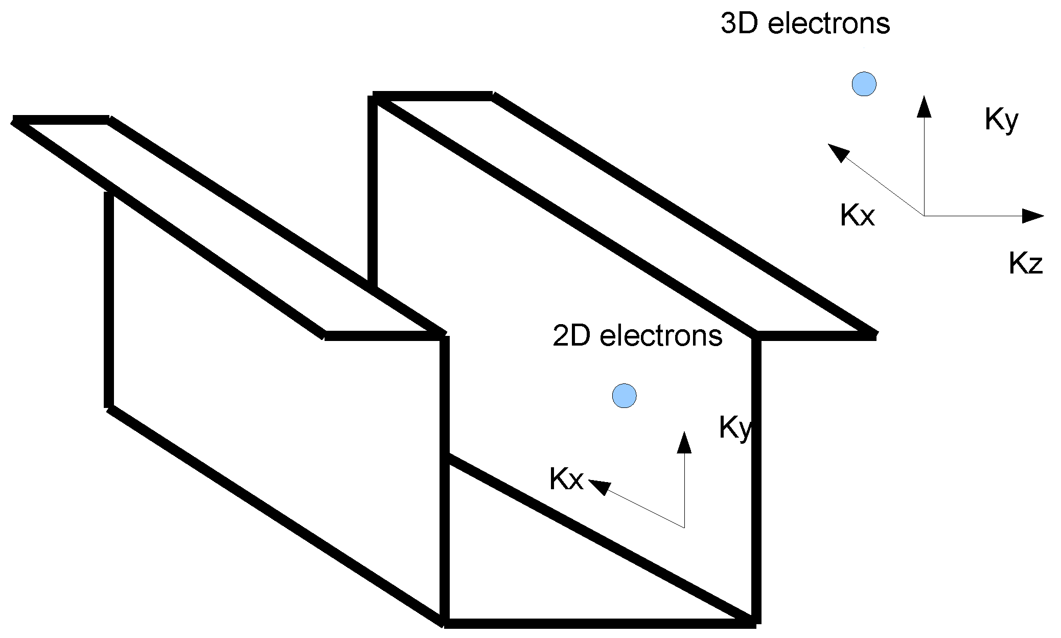
4. Two-Dimensional Electron Gases: The Case of Quantum Confinement

In this section, we consider the case of an ensemble of electrons (the treatment of holes would be analogous) confined along one dimension, called quasi 2Delectron gas (2DEG) [16,18,19,20,
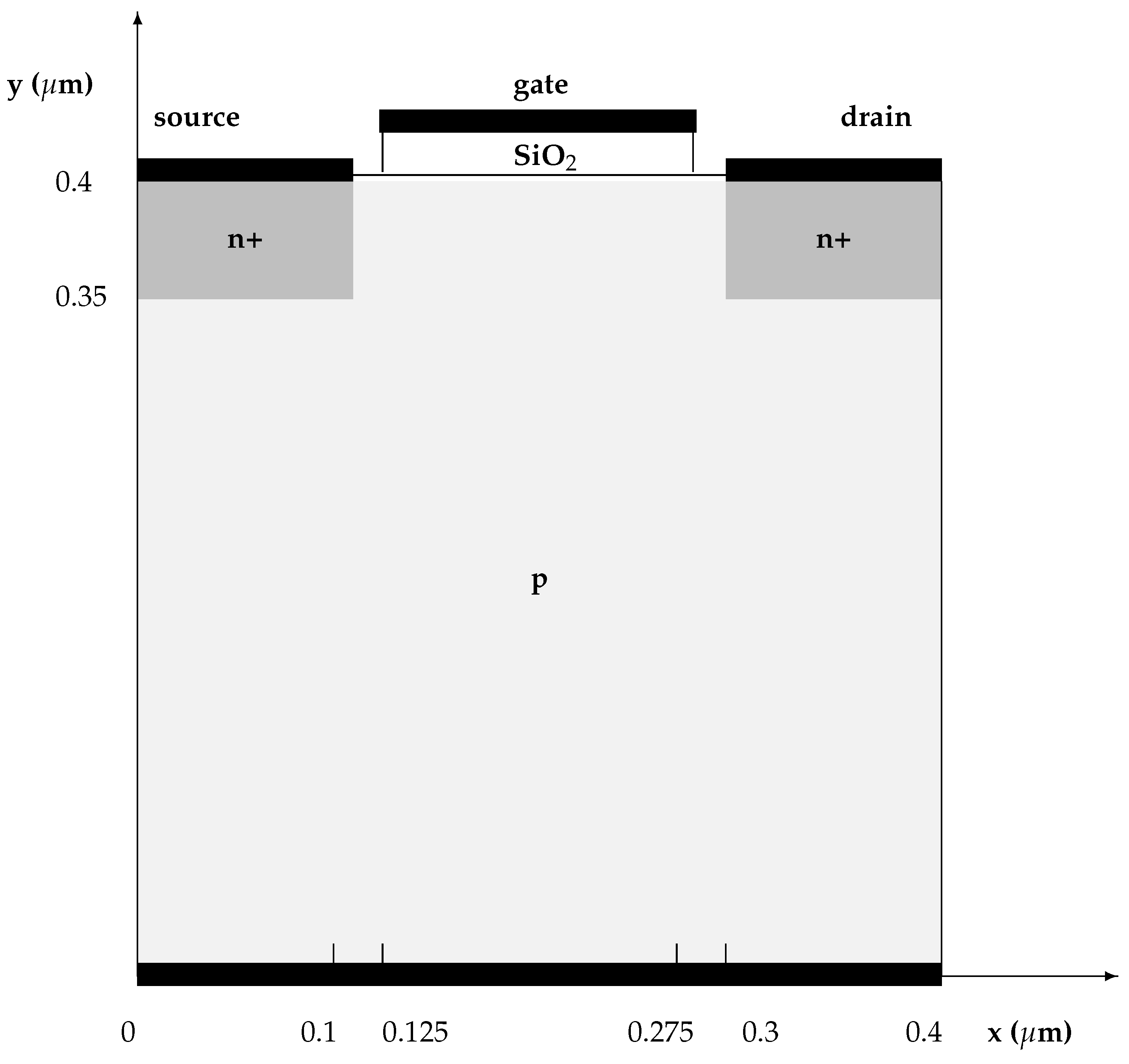
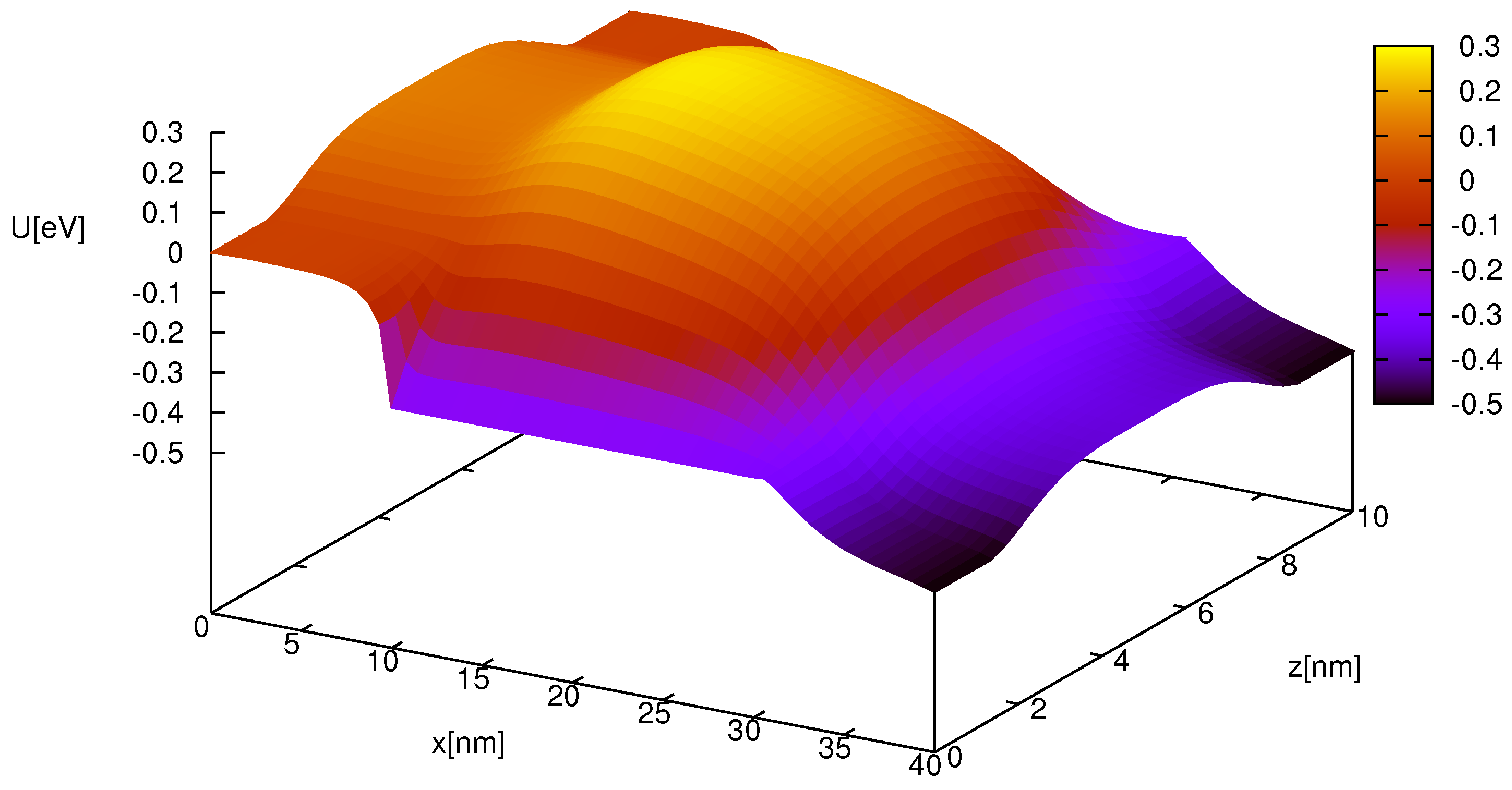
44]. This situation arises when the length scale in one (the confined) space direction of the semiconductor device under study is of the order of de Broglie wavelength of electrons, while the nonconfined directions have a much bigger length scale. In other words, electrons are in a quantum regime in the confined direction and exhibit a classical behaviour in the nonconfined ones [16] as shown in Figure 1.
Let us suppose that electrons are quantized along one direction, which we choose as the z direction, and free to move in the orthogonal x-y plane. Let Ω = [ 0 , L x ] × [ 0 , L y ] × [ 0 , L z ] R 3 be the spatial domain. Here, L x , L y , L z > 0 are fixed. More general cases with a variable confining direction can be easily incorporated.
Let us introduce the parameter σ defined as the ratio between the transversal (perpendicular to the x-y plane) typical length scale L t and the longitudinal typical length scale L l
σ = L t L l
and assume that σ 1 . Moreover, as is customary, let us assume the following ansatz about the electron wave function
ψ ( k , r ) = ψ ( k x , k y , k z , x , y , z ) = 1 A φ ( σ r | | , z ) e i k | | · σ r | | in Ω ,
with k | | = ( k x , k y ) and r | | = ( x , y ) denoting the longitudinal components of the wave-vector k and the position vector r , respectively, and A being the area of the x-y cross-section. The previous wave function is inserted into the stationary Schrödinger equation in the effective mass approximation
2 2 m * Δ + E C ( r ) ψ = E ψ ,
where m * is the electron effective mass, E C is the conduction band minimum, E C = q ( V C + V ) , with V C ( z ) the confining potential and V ( r | | , z ) the self-consistent electrostatic potential.
Under the assumption that the confining potential is so high that it gives rise to a barrier which can be considered infinite, it enters into the equations only through the boundary conditions
ψ ( r | | , z ) = 0 a t z = 0 and z = L z ,
and E C = q V is taken.
Therefore, introducing the slowly varying variable r ˜ | | = σ r | | and inserting (62) into (63), one has
2 2 m * σ 2 Δ r | | φ ( r ˜ | | , z ) + 2 i k | | · r | | φ ( r ˜ | | , z ) k | | 2 φ ( r ˜ | | , z ) 2 2 m * z 2 φ ( r ˜ | | , z ) q V ( r ˜ | | , z ) φ ( r ˜ | | , z ) = E φ ( r ˜ | | , z ) .
In the limit σ 0 + , one formally gets that the envelope function φ must solve the reduced Schrödinger equation
2 2 m * d 2 d z 2 q V ( r | | , z ) φ ( σ r | | , z ) = ε φ ( σ r | | , z ) , 0 z L z ,
with boundary conditions
φ = 0 at z = 0 and z = L z .
The solution of (64) and (65) depends only parametrically on r | | (and in a slow way), and more in general also on time t if a non-steady-state solution is considered. In fact, electrons as waves achieve equilibrium along the confined direction in a time which is much shorter than the typical transport time, so that one can adopt a quasi-static description along the z-direction. The couple (64) and (65) constitutes a one dimensional Sturm–Liouville problem, which admits a countable set of eigen-pairs (subbands) ( φ ν ( r | | , z ) , ε ν ( r | | ) ) , ν = 1 , 2 . . . , whose eigenvalues are simple and do not cross. The potential V is obtained from the Poisson equation
· ( ϵ s V ) = q ( N d ( r ) n ) ,
where the electron density n is given by
n ( r ) = ν = 1 + ρ ν ( r | | ) | φ ν ( r | | , z , ) | 2 ,
with ρ ν the (areal) density of electrons of the νth subband and for simplicity an n–doped material has been considered. Of course, the Schrödinger and Poisson equations are coupled and must be solved simultaneously.
For devices with longitudinal characteristic length of a few tens of nanometers, the transport of electrons in the longitudinal direction is semi-classical within a good approximation. Therefore, electrons in each subband can be considered as different populations, the state of each of them being described by a semiclassical distribution function f ν ( x , y , k x , k y , t ) , and electron transport along the longitudinal direction being determined by adding to the Schrödinger–Poisson system the following system of coupled Boltzmann equations
f ν t + 1 k | | E ν · r | | f ν q E ν e f f · k | | f ν = μ = 1 C ν , μ [ f ν , f μ ] , ν = 1 , 2 ,
where E ν e f f = 1 q r | | ε ν ( r | | ) , and the electron energy in each subband E ν is the sum of a transversal contribution ε ν and a longitudinal one
E ν ( r | | , k | | ) : = ε ν ( r | | ) + ε | | ( k | | ) = ε ν ( r | | ) + 1 2 α 1 + 4 α 2 2 m * k x 2 + k y 2 1 ,
where α is the non-parabolicity parameter. Consequently, the longitudinal electron velocity is
v | | = 1 k | | ε | | = k | | m * 1 + 2 α ε | | .
A formal justification of Equation (67) can be found in [45]. Regarding the collision operator, in the non-degenerate approximation, each contribution has the general form [18,19,20]
C ν , μ [ f ν , f μ ] = 1 ( 2 π ) 2 B 2 w μ ν ( k | | , k | | ) f μ w ν μ ( k | | , k | | ) f ν d 2 k | | ,
where B 2 is the two-dimensional Brillouin zone. When μ = ν , the scattering is intra-subband; when μ ν , it is the inter-subband. We recall that inter-subband transitions may also happen in the absence of phonons, by quantum mechanical tunneling induced by the presence of a static field as has been shown for example in [46]. The term w μ ν ( k | | , k | | ) is the transition rate from the longitudinal state with wave-vector k | | , belonging to the μth subband, to the longitudinal state with wave-vector k | | , belonging to the νth subband, and f μ f μ ( r | | , k | | , t ) . In Si, the relevant 2D scattering mechanisms are the acoustic phonon scattering, and the non-polar optical phonon scattering. Their expressions are the 2D version of those shown in Section 2 and can be found in [18,19,20,47]. Attempts to directly solve the Schrödinger–Poisson–Boltzmann system can be found, for example, in [16,17,48] where numerical schemes based on finite differences have been employed. However, the direct numerical approach is a daunting computational task and requires very long computing times. This has again prompted the development of simpler macroscopic models for CAD purposes. These models can be obtained as moment equations of the Boltzmann transport equations under suitable closure relations [18,19,20]. The moment of the ν-th subband distribution with respect to a weight function a ( k | | ) reads
M a , ν = B 2 a ( k | | ) f ν ( r | | , k | | , t ) d 2 k | | .
In particular, analogously to the previous cases, we take as basic moments
the   areal   density ρ ν = B 2 f ν ( r | | , k | | , t ) d 2 k | | ,
the   longitudinal   mean   velocity V ν = 1 ρ ν B 2 v | | f ν ( r | | , k | | , t ) d 2 k | | ,
the   longitudinal   mean   energy W ν = 1 ρ ν B 2 ε | | f ν ( r | | , k | | , t ) d 2 k | | ,
the   longitudinal   mean   energy-flux S ν = 1 ρ ν B 2 ε | | v | | f ν ( r | | , k | | , t ) d 2 k | | .
The corresponding moment system reads
ρ ν t + r | | · ( ρ ν V ν ) = ρ ν μ C ρ , ν μ ,
( ρ ν V ν ) t + r | | · ( ρ ν F ν ( 0 ) ) + ρ ν G ν ( 0 ) r | | ε ν = ρ ν μ C V , ν μ ,
( ρ ν W ν ) t + r | | · ( ρ ν S ν ) + ρ ν r | | ε ν · V ν = ρ ν μ C W , ν μ ,
( ρ ν S ν ) t + r | | · ( ρ ν F ν ( 1 ) ) + ρ ν G ν ( 1 ) r | | ε ν = ρ ν μ C S , ν μ ,
where
F ν ( 0 ) F ν ( 1 ) = 1 ρ ν B 2 1 ε | | v | | v | | f ν ( r | | , k | | , t ) d 2 k | | ,
G ν ( 0 ) G ν ( 1 ) = 1 ρ ν B 2 1 k | | v | | 1 k | | ε | | v | | f ν ( r | | , k | | , t ) d 2 k | | ,
C ρ , ν μ C W , ν μ = 1 ρ ν B 2 1 ε | | w μ ν ( k | | , k | | ) f μ w ν μ ( k | | , k | | ) f ν d 2 k | | d 2 k | | ,
C V , ν μ C S , ν , μ = 1 ρ ν B 2 v | | ε | | v | | w μ ν ( k | | , k | | ) f μ w ν μ ( k | | , k | | ) f ν d 2 k | | d 2 k | | .
Also in this case, the above written fluxes and production terms are extra-variables for which closure relations are needed. In order to employ MEP, a suitable expression of the entropy for the system under consideration has to be found. Neglecting the mutual interaction of electrons in different subbands, considering the phonon gas as a thermal bath and assuming the electron gas is sufficiently dilute, in each subband the expression of the entropy is the semiclassical limit of that arising from the Fermi statistics. Eventually, for obtaining the total entropy, one has to consider that electrons have a quantum behaviour along the z-direction, therefore we define the entropy density of the system as
S [ f 1 , f 2 , ] = k B ν = 1 + | φ ν ( r | | , z , t ) | 2 quantum   effect B 2 f ν log ( 2 π 2 f ν ) f ν d 2 k | | semiclassical   contribution .
Remark 7.
The proposed expression of the entropy has been introduced for the first time in [20,47]. It combines quantum effects and semiclassical transport along the longitudinal direction, weighting the contribution of each subband with the square modulus of the φ ν ( z , t ) ’s arising from the Schrödinger–Poisson block.
According to MEP, the f ν ’s are estimated by means of the distributions f ν M E P ’s that r | | [ 0 , L x ] × [ 0 , L y ] , t > 0 , solve the problem:
max f 1 ( r | | , · , t ) F 2 D f 2 ( r | | , · , t ) F 2 D S [ f 1 , f 2 , ] under   the   constraints M a A , ν = B 2 a A ( k | | ) f ν ( r | | , k | | , t ) d 2 k | | ,
where the M a A , ν ’s are the basic moments (69)–(72) and F 2 D is the space of the summable function with respect to k | | such that the moments appearing in the system (73)–(76) exist.
With the above choice of the functions a A ( k | | ) = ( 1 , v | | , ε | | , ε | | v | | ) , the resulting maximum entropy distribution functions read (the factor k B has been included into the multipliers)
f ν M E P = exp λ ν + λ V , ν · v | | + λ W , ν + λ S , ν · v | | ε | | .
In order to complete the procedure, similarly to the previous case, one has to insert the f ν M E P ’s into the constraints (69)–(72) and express the Lagrange multipliers as functions of the basic moments ρ ν , V ν , W ν , S ν . In general, in the case considered in this section as well as in that considered in Section 2, it is not possible to assure that such a procedure can be accomplished. The solvability of the MEP problem depends on the band structure and on the choice of the moments, as well known already in gas-dynamics [14,49]. For example, if the parabolic case (where the energy is a quadratic function of the wave vector) is considered, the same drawbacks of classical gas-dynamics arise regarding the lack of integrability of the MEP distribution function. In the case of the Kane dispersion relation, the solvability of the MEP problem is guaranteed by the following property, proven in [49].
Proposition 3.
When the Kane model for the energy band is employed, the corresponding maximum entropy models are symmetric hyperbolic systems with convex domains of definition and the equilibria are interior points, guaranteeing the validity of expansions around equilibrium states.
The proof has been given for a 3D electron gas, but it can be extended to a 2DEG in a straightforward way.
For the 2DEG case, the final expressions of the extra-fluxes and production terms, obtained by using linearized MEP distribution functions, can be found in [18,47] for the parabolic approximation and in [19,20] for the non-parabolic one. The resulting moment system has been used to simulate double-gate MOSFETs in [18,19].

5. Some Numerical Simulations

In this last section, we present some of the numerical results obtained by implementing the models sketched in the previous sections. The information concerning the numerical schemes will be skipped. The interested readers are referred to the indicated papers. For optimization of electron devices using the models presented above, see [50] and references therein.

5.1. p-n Junction

The full model for holes and electrons, presented in Section 2, has been used for the numerical simulation of a Si p-n junction diode with a doping profile given by [22]
N d ( x ) N a ( x ) = c 0 if 0 < x < L 0 c 0 if L 0 < x < L ,
with an abrupt junction at L 0 . The physical parameters of the device are reported in Table 1. The numerical solution has been obtained by resorting to an extension [51] of the traditional central differencing scheme for one-dimensional balance laws with (possibly stiff) source terms, which has been developed on the basis of the Nessyhau and Tadmor scheme [52] for homogeneous hyperbolic systems.
The bias voltage at the contacts is the superposition of the thermal equilibrium boundary potential (the built in potential V b i ) and the applied potential V a . In Figure 2 and Figure 3, the stationary carrier densities and the electrostatic potential are shown for the following applied voltages: V a = 0.2 , 0 , 0.75 , 1 V, the sign + referring to direct polarization.

5.2. Simulation of a MESFET

In this subsection, we show the simulation of a bi-dimensional Metal Semiconductor Field Effect Transistor (MESFET) made with the MEP model. The numerical method is based on the discretization proposed in [53].
The shape of the device is pictured in Figure 4. The device has a 0.4 μ m channel. The source and drain lengths are 0.1 μ m and the contact at the gate is 0.2 μ m long. The distance between the gate and the other two contacts is 0.1 μ m. The lateral subdiffusion of the source and the drain region is about 0.05 μ m. The same doping concentration C ( x ) as in [53] is considered
C ( x ) = n + = 3 × 10 17 cm 3 in   the n + region n = 10 17 cm 3 in   the n region
with abrupt junctions. We take a reference frame with axes parallel to the edges of the device. The numerical domain representing the MESFET is
Ω = [ 0 , 0.6 ] × [ 0 , 0.2 ]
where the unit length is the micron.
The regions of high doping n + are the subset
[ 0 , 0.1 ] × [ 0.15 , 0.2 ] [ 0.5 , 0.6 ] × [ 0.15 , 0.2 ] .
Γ D represents the source, gate and drain
Γ D = ( x , y ) : y = 0.2 , 0 x 0.1 , 0.2 x 0.4 , 0.5 x 0.6 .
The remaining part of Ω is Γ N . The boundary conditions are assigned as follows. We have ohmic contacts at the source and drain:
n = n + , W = 3 2 k B T L , V = Φ b at   drain 0 at   source .
At the gate we have a Schottky contact
n = n g , W = 3 2 k B T L , V = Φ g .
Indeed, the potential at the contacts should include the built-in potential and the density at the gate should be related to the potential. Here, we do not enter into the details of the modeling of the Schottky contacts and, by using the invariance of the electric field with respect to changes of the potential for additive constants, we choose as in [54]
n g = 3.9 × 10 5 cm 3 , Φ g = 0.8 V
In the remaining part Γ N of the boundary, we have
ν · n = 0 , ν · W = 0 , ν · V = 0 .
Here, ∇ is the bi-dimensional gradient operator while ν is the unit outward normal vector to Ω in the considered points.
A uniform mesh has been used with 33 × 97 grid points. The stationary solution is reached after about 5 picoseconds. The numerical results are shown in Figure 5, Figure 6, Figure 7 and Figure 8. The typical depletion region close to the gate with the presence of steep gradients is numerically well described.

5.3. Simulation of a MOSFET

The Metal Oxide Semiconductor Field Effect Transistor (MOSFET) is a largely used device in modern electronics. The same mathematical model and numerical scheme as for the MESFET is adopted; the shape of the device is pictured in Figure 9. The device has a 0.2 μ m channel. The source and drain lengths are 0.1 μ m and the contact at the gate is 0.15 μ m long. The distance between the gate and the other two contacts is 0.025 μ m. The lateral subdiffusion of the source and the drain region is about 0.05 μ m. The gate oxide is 0.15 μ m long and 20 nm thick. Of course, smaller devices can be considered without any substantial modification to the used approach.
The doping concentration is
C ( x ) = n + = 10 17 cm 3 in the n + regions p = 10 14 cm 3 in the p region
with abrupt junctions.
At variance with MESFET, there are different built-in potentials which we explicitly take into account by using the simple model
Φ b D = Φ b S = k B T L q ln n + n i
at drain and source,
Φ b B = k B T L q ln p n i
at bulk contact. Here, n i is the intrinsic electron concentration ( 10 10 cm 3 ). The reference axes are chosen parallel to the edges of the device. The silicon part of the MOSFET is represented by the numerical domain
[ 0 , 0.4 ] × [ 0 , 0.4 ]
and at the top of the silicon part the silicon oxide domain is
[ 0.125 , 0.275 ] × [ 0.4 , 0.42 ]
where the unit length is the micron.
The regions of high-doping n + are the subset
[ 0 , 0.1 ] × [ 0.35 , 0.4 ] [ 0.3 , 0.4 ] × [ 0.35 , 0.4 ] .
A uniform mesh of 64 × 64 grid points has been used in the silicon part. The Poisson equation is solved on the entire (silicon and oxide) domain. Of course, in the oxide, the Poisson equation becomes the Laplace one.
We have assumed ohmic contacts at the source, drain, gate and bulk contacts, to be homogeneous Neumann conditions on the remaining part of the boundary. The surface charge at the oxide interface is neglected and the continuity of the electric potential and electric field is imposed. The values of density and energy at the interface are obtained by the interior grid points with a linear interpolation in the direction orthogonal to the boundary.
In order to reach the desired bias, we have needed to resort to a continuation method on applied potential. First, we iterate with respect to the difference of the built-in potential between drain and bulk contacts, keeping at zero V D S . Then, we iterate with respect to the drain–gate potential and finally we increase the drain–source potential.
All the main features of the electron dynamics are well described, in particular the charge accumulation beside the oxide, and the pronounced depletion at the drain contact due to the strong electric field.
Again, the density current presents a singularity at the first edge of the drain and therefore we evaluated the current by considering, as for MESFET, the regularization from the interior.
As for the MESFET device, current gain and miniaturization are crucial tasks to take into account when designing this kind of device. However, miniaturization plays a crucial role for MOSFETs for various reasons; first, a shorter MOSFET helps the current flow, since a small device decreases the resistance. Second, a small MOSFET helps in reducing gate capacity and, in general, to have a faster switch on/off operation. The numerical results are presented in Figure 10, Figure 11 and Figure 12.

5.4. Simulation of a DG-MOSFET

The 2DEG model, illustrated in Section 4, has been employed to simulate the nanoscale silicon DG-MOSFET represented in Figure 13, including the non-parabolicity effects [18,19]. The length of the diode is L x = 40 nm, the width of the silicon layer is L z = 8 nm and the thickness of each oxide layer is t o x = 1 nm. The highly doped n + regions are 10 nm long. The gate contacts have the same length as the n region and are above it. The device is supposed to be infinite in the y direction.
The doping in the n + regions is N d ( x ) = N d + = 10 20 cm 3 and in the n region is N d ( x ) = N d = 10 15 cm 3 , with a regularization at the two junctions by a hyperbolic tangent profile
N d ( x ) = N d + d tanh x x 1 s tanh x x 2 s ,
where s = 0.2 nm, d = N d + 2 1 N d N d + , x 1 = 10 nm and x 2 = 30 nm.
Due to the symmetries and dimensions of the device, the transport is, within a good approximation, one dimensional and along the longitudinal direction with respect to the two oxide layers, while the electrons are quantized in the transversal direction. The oxide gives rise, with a good approximation, to an infinitely deep potential barrier; in fact, realistic values of the potential barrier are more than 3 eV high and it is very unlikely to find electrons with such an energy in the device under consideration. Six equivalent valleys are considered with a single effective mass m * = 0.32 m e . For details about the appropriate boundary and initial conditions, as well as the numerical method, the interested reader is referred to [18,19]. The numerical experiments indicate that it is sufficient to take into account only the first three subbands.
As the first case, a symmetric situation with V D = 0.5 V and V g l = V g u = 3 V is considered, where V D is the voltage applied at the drain with respect to that at the source, and V g l and V g u are the voltages applied at the lower and the upper gate, respectively. In Figure 14 and Figure 15, the steady state density and the potential are plotted. The solution does not present any spurious oscillation or boundary layer and reflects the symmetry of the problem.
As the second case, V D = 0.5 V, V g l = 3 V and V g u = 3 V are taken. In Figure 16 and Figure 17, the density and the potential are respectively plotted, while in Figure 18b the first three subband bottoms are shown. One can note the depletion region beneath the upper gate.
In Figure 18, the first three subband bottoms are shown. There is a good qualitative agreement with the other numerical simulations known in the literature [17].
From Figure 19, a very accurate current conservation is evident, proving the robustness of the numerical method. In the second case, the current is reduced by one half, due to the gate voltage in agreement with the behaviour of the density. The areal density, the average velocity and the energy measured from the subband bottom, and the current in the first three subbands are shown in Figure 20, Figure 21 and Figure 22. The areal density is not symmetrical between the source and drain within each subband but the total areal density is so.
The drift (mean) velocity has been evaluated according to the formula
V = ν ρ ν V ν μ ρ μ .
Similarly, the global longitudinal mean energy has been evaluated taking as reference value the bottom of the first subband according to the formula
W = ν ρ ν W ν + ε ν ε 1 μ ρ μ .
The maximum drift velocity in the channel is one and half times the saturation velocity when V g l = V g u = 3 V, while it is about two times the saturation velocity when V g l = 3 V and V g u = 3 V. Moreover, in the first case, the velocity in the first subband is lower than that in the first subband in the second case. Instead, the velocity in the second and the third subbands is higher in the first case, but with a resulting total longitudinal current which is lower. The energy has an evidently different value between the source and drain as happens in the semiclassical case.
Eventually, the characteristic curves are shown in Figure 23 by fixing V g l = 3 V and varying V g u from −3 V to 3 V. With increasing V g u , the average longitudinal current increases as a consequence of the controlling effect of the gate voltage on the electric characteristics of the device.

6. Conclusions

A review on the exploitation of the Maximum Entropy Principle in the formulation of macroscopic models able to describe the charge and heat transport in semiconductor devices has been presented. The models are obtained starting from the Boltzmann transport equations for the charge and the phonon distribution functions, by taking—as macroscopic variables—suitable moments of the distributions and resorting to MEP in order to close the evolution equations for the chosen moments. Firstly, semiclassical models have been reviewed and eventually an approach to also take into account quantum effects has been shown. The latter consists of using the moment system arising from the Wigner equation.
In the cases where quantum effects are relevant only along one direction, another strategy has been introduced. A quasi-static description has been adopted, based on a coupled Schrödinger–Poisson system, along the confining direction, leading to a subband decomposition of the electron energy levels, while the transport along the longitudinal directions is described by a semiclassical Boltzmann equation for each subband.
Several physical situations, which have been investigated in the last two decades, have been reported in the paper. For the sake of conciseness, some further applications have been omitted. A MEP based model for 2D–3D electron gases, of particular interest in the simulation of nanoscale MOSFET, can be found in [55]. A hydrodynamical model for charge transport in graphene has been formulated in [56,57].
Apparently, MEP is revealed to be a sound method for devising, in a systematic way, macroscopic models, e.g., energy–transport and hydrodynamical ones, which are less complex to tackle numerically but still retain a good accuracy with respect to the results based on the direct solutions of the transport equations.

Acknowledgments

The author Vittorio Romano acknowledges the financial support by the project FIR 2014 Charge Transport in Graphene and Low Dimensional Structures: Modeling and Simulation, University of Catania, Italy.

Author Contributions

Both authors have jointly worked to the manuscript with an equal contribution. Both authors have read and approved the final manuscript.

Conflicts of Interest

The authors declare no conflict of interest.

Abbreviations

The following abbreviations are used in this manuscript:
MEPMaximum Entropy Principle
BTEBoltzmann Transport Equation
CADComputer Aided Design
DG-MOSFETDouble Gate Metal Oxide Semiconductor Field Effect Transistors
BBPBoltzmann–Bloch–Peierls

References

  1. Jacoboni, C. Theory of Electron Transport in Semiconductors: A Pathway from Elementary Physics to Nonequilibrium Green Functions; Springer: Berlin/Heidelberg, Germany, 2010. [Google Scholar]
  2. Carrillo, J.A.; Majorana, A.; Vecil, F. A semi-Lagrangian deterministic solver for the semiconductor Boltzmann-Poisson system. Commun. Comput. Phys. 2007, 2, 1027–1054. [Google Scholar]
  3. Baccarani, G.; Wordeman, M.R. An investigation on steady-state velocity overshoot in silicon. Solid State Electron. 1982, 29, 970–977. [Google Scholar] [CrossRef]
  4. Blotekjaer, K. Transport equations for electron in two-valley semiconductors. IEEE Trans. Electron. Devices 1970, 17, 38–47. [Google Scholar] [CrossRef]
  5. Hänsch, W. The Drift-Diffusion Equation and Its Applications in MOSFET Modeling; Springer: Berlin/Heidelberg, Germany, 1991. [Google Scholar]
  6. Dreyer, W.J. Maximisation of the entropy in non-equilibrium. Phys. A Math. Gen. 1987, 20, 6505. [Google Scholar] [CrossRef]
  7. Dreyer, W.J.; Struchtrup, H. Heat pulse experiment revisited. Contin. Mech. Thermodyn. 1993, 5, 3–50. [Google Scholar] [CrossRef]
  8. Alì, G.; Mascali, G.; Romano, V.; Torcasio, C.R. A Hydrodynamical Model for Covalent Semiconductors with Applications to GaN and SiC. Acta Appl. Math. 2012, 122, 335–348. [Google Scholar]
  9. Alì, G.; Mascali, G.; Romano, V.; Torcasio, C.R. A Hydrodynamic Model for covalent semiconductors with a generalized energy dispersion relation. Eur. J. Appl. Math. 2014, 25, 255–276. [Google Scholar] [CrossRef]
  10. Anile, A.M.; Romano, V. Non parabolic band transport in semiconductors: Closure of the moment equations. Contin. Mech. Thermodyn. 1999, 11, 307–325. [Google Scholar] [CrossRef]
  11. Mascali, G.; Trovato, M. A non-linear determination of the distribution function of degenerate gases with an application to semiconductors. Physica A 2002, 310, 121–138. [Google Scholar] [CrossRef]
  12. Muscato, O.; Di Stefano, V. Modeling heat generation in a sub-micrometric n+nn+ silicon diode. J. Appl. Phys. 2008, 104, 124501. [Google Scholar] [CrossRef]
  13. Muscato, O.; Di Stefano, V. Local equilibrium and off-equilibrium thermoelectric effects in silicon semiconductors. J. Appl. Phys. 2011, 110, 093706. [Google Scholar] [CrossRef]
  14. Levermore, C.D. Moment Closure Hierarchies for kinetic Theories. J. Stat. Phys. 1996, 83, 1021–1167. [Google Scholar] [CrossRef]
  15. Romano, V. Quantum corrections to the semiclassical hydrodynamical model of semiconductors based on the maximum entropy principle. J. Math. Phys. 2007, 48, 123504. [Google Scholar] [CrossRef]
  16. Polizzi, E.; Ben Abdallah, N. Subband decomposition approach for the simulation of quantum electron transport in nanostructures. J. Comput. Phys. 2004, 202, 150–180. [Google Scholar] [CrossRef]
  17. Ben Abdallah, N.; Caceres, M.J.; Carrillo, J.A.; Vecil, F. A deterministic solver for a hybrid quantum-classical transport model in nanoMOSFETs. J. Comput. Phys. 2009, 228, 6553–6571. [Google Scholar] [CrossRef]
  18. Camiola, V.D.; Mascali, G.; Romano, V. Numerical Simulation of a Double-Gate Mosfet with a Subband Model for Semiconductors Based on the Maximum Entropy Principle. Contin. Mech. Thermodyn. 2012, 24, 417–436. [Google Scholar] [CrossRef]
  19. Camiola, V.D.; Mascali, G.; Romano, V. Simulation of a double-gate MOSFET by a non-parabolic energy-transport model for semiconductors based on the maximum entropy principle. Math. Comput. Model. 2013, 58, 321–343. [Google Scholar] [CrossRef]
  20. Mascali, G.; Romano, V. A non parabolic hydrodynamical subband model for semiconductors based on the maximum entropy principle. Math. Comput. Model. 2012, 55, 1003–1020. [Google Scholar] [CrossRef]
  21. Mascali, G.; Romano, V. A hydrodynamical model for hole transport in silicon semiconductors: The case of non-parabolic warped bands. Math. Comput. Model. 2011, 53, 213–229. [Google Scholar] [CrossRef]
  22. Mascali, G.; Romano, V. A hydrodynamical model for hole transport in silicon semiconductors: The case of parabolic warped bands. Compel 2012, 31, 552–582. [Google Scholar] [CrossRef]
  23. Mascali, G. A hydrodynamical model for silicon semiconductors includind crystal heating. Eur. J. Appl. Math. 2015, 26, 477–496. [Google Scholar] [CrossRef]
  24. Auer, C.; Schürrer, F.; Koller, W. A semicontinuous formulation of the Bloch–Boltzmann–Peierls equations. SIAM J. Appl. Math. 2004, 64, 1457–1475. [Google Scholar] [CrossRef]
  25. González, P.; Carrillo, J.A.; Gámiz, F. Deterministic Numerical Simulation of 1d kinetic descriptions of Bipolar Electron Devices’. In Scientific Computing in Electrical Engineering, Series: Mathematics in Industry, Subseries: The European Consortium for Mathematics in Industry; Anile, A.M., Alì, G., Mascali, G., Eds.; Springer: Berlin/Heidelberg, Germany, 2006; pp. 339–344. [Google Scholar]
  26. Mascali, G. Maximum entropy principle in relativistic radiation hydrodynamics II: Compton and double Compton scattering. Contin. Mech. Thermodyn. 2002, 14, 549. [Google Scholar] [CrossRef]
  27. Anile, A.M.; Mascali, G. Theoretical foundations for tail electron hydrodynamical models in semiconductors. Appl. Math. Lett. 2001, 14, 245–252. [Google Scholar] [CrossRef]
  28. Morandi, O.; Barletti, L. Particle dynamics in graphene: Collimated beam limit. J. Comput. Theor. Transp. 2015, 43, 418–432. [Google Scholar] [CrossRef]
  29. La Rosa, S.; Mascali, G.; Romano, V. Exact maximum entropy closure of the hydrodynamical model for Si semiconductors: The 8-moment case. SIAM J. Appl. Math. 2009, 70, 710–734. [Google Scholar] [CrossRef]
  30. Romano, V. Non parabolic band transport in semiconductors: Closure of the production terms in the moment equations. Contin. Mech. Thermodyn. 2000, 12, 31–51. [Google Scholar] [CrossRef]
  31. Mascali, G. A new formula for thermal conductivity based on a hierarchy of hydrodynamical models. J. Stat. Phys. 2016, 163, 1268–1284. [Google Scholar] [CrossRef]
  32. Jaynes, E.T. Information Theory and Statistical Mechanics. Phys. Rev. B 1957, 106, 620. [Google Scholar] [CrossRef]
  33. Wu, N. The Maximum Entropy Method; Springer: Berlin/Heidelberg, Germany, 1997. [Google Scholar]
  34. Degond, P.; Ringhofer, C. Quantum moment hydrodynamics and the entropy principle. J. Stat. Phys. 2003, 112, 587–628. [Google Scholar] [CrossRef]
  35. Degond, P.; Méhats, F.; Ringhofer, C. Quantum energy-transport and drift-diffusion models. J. Stat. Phys. 2005, 118, 625–627. [Google Scholar] [CrossRef]
  36. Barker, J.; Ferry, D. Self-Scattering Path-Variable Formulation of High-Field, Time-Dependent, Quantum Kinetic Equations for Semiconductor Transport in the Finite-Collision-Duration Regime. Phys. Rev. Lett. 1979, 42, 1779. [Google Scholar] [CrossRef]
  37. Fromlet, F.; Markowich, P.A.; Ringhofer, C. A Wigner function Approach to Phonon Scattering. VLSI Des. 1999, 9, 339–350. [Google Scholar] [CrossRef] [PubMed]
  38. Camiola, V.D.; Romano, V. Quantum BGK model for electron transport in semiconductors. In Proceedings of the 15th Conference on Waves and Stability in Continuous Media, Palermo, Italy, 28 June–1 July 2009.
  39. Romano, V. The equilibrium Wigner function in the case of nonparabolic energy band. In Progress in Industrial Mathematics at ECMI 2008; Fitt, A.D., Norbury, J., Ockendon, H., Wilson, E., Eds.; Springer: Berlin/Heidelberg, Germany, 2010; Volume 15, pp. 135–140. [Google Scholar]
  40. Majorana, A. Space homogeneous solutions of the Boltzmann equation describing electron-phonon interactions in semiconductors. Transp. Theory Stat. Phys. 1991, 20, 261–279. [Google Scholar] [CrossRef]
  41. Majorana, A. Conservation laws from the Boltzmann equation describing electron-phonon interactions in semiconductors. Transp. Theory Stat. Phys. 1993, 22, 849–859. [Google Scholar] [CrossRef]
  42. Majorana, A. Equilibrium solutions of the non-linear Boltzmann equation for an electron gas in a semiconductor. Il Nuovo Cimento B 1993, 108, 871–877. [Google Scholar] [CrossRef]
  43. Gardner, C. The quantum hydrodynamic model for semiconductor devices. SIAM J. Appl. Math. 1994, 54, 409–427. [Google Scholar] [CrossRef]
  44. Muscato, O.; Castiglione, T. A Hydrodynamic Model for Silicon Nanowires Based on the Maximum Entropy Principle. Entropy 2016, 18, 368. [Google Scholar] [CrossRef]
  45. Camiola, V.D.; Mascali, G.; Romano, V. The Moment Method for Charge Transport in Low Dimensional Semiconductor Devices; Springer: Berlin/Heidelberg, Germany, 2017; in press. [Google Scholar]
  46. Morandi, O. Multiband Wigner-function formalism applied to the band to band transition phenomena. Phys. Rev. B 2009, 80, 024301. [Google Scholar] [CrossRef]
  47. Mascali, G.; Romano, V. Hydrodynamic subband model for semiconductors based on the maximum entropy principle. Nuovo Cimento C 2010, 33, 155–163. [Google Scholar]
  48. Galler, M.; Schuerrer, F. A deterministic Solver to the Boltzmann-Poisson System Including Quantization Effects for Silicon-MOSFETs. In Progress in Industrial Mathematics at ECMI 2006, Series: Mathematics in Industry; Springer: Berlin/Heidelberg, Germany, 2008; pp. 531–536. [Google Scholar]
  49. Junk, M.; Romano, V. Maximum entropy moment system of the semiconductor Boltzmann equation using Kane dispersion relation. Contin. Mech. Thermodyn. 2005, 17, 247–267. [Google Scholar] [CrossRef]
  50. Straquadanio, G.; Romano, V.; Nicosia, G. Semiconductor device design using the BIMADS algorithm. J. Comput. Phys. 2013, 242, 304–320. [Google Scholar] [CrossRef]
  51. Liotta, S.F.; Romano, V.; Russo, G. Central schemes for balance laws of relaxation type. SIAM J. Numer. Anal. 2000, 38, 1337–1356. [Google Scholar] [CrossRef]
  52. Nessyahu, H.; Tadmor, E. Non-oscillatory central differencing for hyperbolic conservation law. J. Comput. Phys. 1990, 87, 408–463. [Google Scholar] [CrossRef]
  53. Romano, V. 2D Simulation of a Silicon MESFET with a Nonparabolic Hydrodynamical Model Based on the Maximum Entropy Principle. J. Comput. Phys. 2002, 176, 70–92. [Google Scholar] [CrossRef]
  54. Chen, Z.; Cockburn, B.; Jerome, J.; Shu, C.-W. Finite element computation of the hydrodynamic model of semiconductor devices. VLSI Des. 1995, 3, 145–158. [Google Scholar] [CrossRef]
  55. Camiola, V.D.; Romano, V. 2DEG-3DEG charge transport model for MOSFET based on the maximum entropy principle. SIAM J. Appl. Math. 2013, 73, 1439–1459. [Google Scholar] [CrossRef]
  56. Camiola, V.D.; Romano, V. Hydrodynamical Model for Charge Transport in Graphene. J. Stat. Phys. 2014, 157, 1114–1137. [Google Scholar] [CrossRef]
  57. Coco, M.; Majorana, A.; Mascali, G.; Romano, V. Comparing kinetic and hydrodynamical models for electron transport in monolayer graphene. In Proceedings of the VI International Conference on Computational Methods for Coupled Problems in Science and Engineering, Coupled Problems 2015, Venice, Italy, 18–20 May 2015.
Figure 1. Schematic representation of electron confinement in one dimension due to a potential barrier.
Entropy 19 00036 g001
Figure 2. (a,c) Densities and electric potential for V a = 0.2 V, electrons (continuous line), total holes (dashed line) and heavy holes (dashed–dotted line); (b,d) Densities and electric potential for V a = 0 , electrons (continuous line), total holes (dashed line) and heavy holes (dashed–dotted line).
Entropy 19 00036 g002
Figure 3. (a,c) Densities and electric potential for V a = 0.75 V, electrons (continuous line), total holes (dashed line) and heavy holes (dashed–dotted line); (b,d) Densities and electric potential for V a = 1 V, electrons (continuous line), total holes (dashed line) and heavy holes (dashed–dotted line).
Entropy 19 00036 g003
Figure 4. Schematic representation of a bidimensional MESFET.
Entropy 19 00036 g004
Figure 5. Stationary charge density in the MESFET in the case Φ b = 1 V.
Entropy 19 00036 g005
Figure 6. Stationary energy per charge carrier in the MESFET in the case Φ b = 1 V.
Entropy 19 00036 g006
Figure 7. Stationary velocity of the carriers in the MESFET in the case Φ b = 1 V.
Entropy 19 00036 g007
Figure 8. Stationary electric potential in the MESFET in the case Φ b = 1 V.
Entropy 19 00036 g008
Figure 9. Schematic representation of a bidimensional MOSFET.
Entropy 19 00036 g009
Figure 10. Stationary electron density in the MOSFET in the case V b = 1 V and V g = 0.8 V.
Entropy 19 00036 g010
Figure 11. Stationary energy per charge carrier in the MOSFET in the case V b = 1 V and V g = 0.8 V.
Entropy 19 00036 g011
Figure 12. Stationary electric potential in the MOSFET in the case V b = 1 V and V g = 0.8 V.
Entropy 19 00036 g012
Figure 13. Simulated double gate MOSFET. Along the y axis, the device is considered as infinite.
Entropy 19 00036 g013
Figure 14. Stationary density in the case V D = 0.5 V and V g l = V g u = 3 V.
Entropy 19 00036 g014
Figure 15. Stationary electrostatic potential energy in the case V D = 0.5 V and V g l = V g u = 3 V.
Entropy 19 00036 g015
Figure 16. Stationary density in the case V D = 0.5 V and V g l = 3 V, V g u = 3 V.
Entropy 19 00036 g016
Figure 17. Stationary electrostatic potential energy in the case V D = 0.5 V and V g l = 3 V, V g u = 3 V.
Entropy 19 00036 g017
Figure 18. First three subbands at the steady state in the case V D = 0.5 V and V g l = V g u = 3 V (a); V D = 0.5 V and V g l = 3 V, V g u = 3 V (b).
Entropy 19 00036 g018
Figure 19. Average areal current in the first three subbands and global areal current in the case V D = 0.5 V and V g l = V g u = 3 V (a); V D = 0.5 V and V g l = 3 V, V g u = 3 V (b).
Entropy 19 00036 g019
Figure 20. Areal density in the first three subbands in the case V D = 0.5 V and V g l = V g u = 3 V (a); V D = 0.5 V and V g l = 3 V, V g u = 3 V (b).
Entropy 19 00036 g020
Figure 21. Average velocity in the first three subbands and global mean velocity in the case V D = 0.5 V and V g l = V g u = 3 V (a); V D = 0.5 V and V g l = 3 V, V g u = 3 V (b).
Entropy 19 00036 g021
Figure 22. Average total energy measured from the bottom of the first subband W ν + ε ν ε 1 in the first three subbands and global mean energy in the case V D = 0.5 V and V g l = V g u = 3 V (a); V D = 0.5 V and V g l = 3 V, V g u = 3 V (b).
Entropy 19 00036 g022
Figure 23. Longitudinal mean current (A/cm) versus the source–drain voltage V D witht V g l = 3 V and V g u ranging from −3 V to +3 V according to the arrow.
Entropy 19 00036 g023
Table 1. Physical parameters of the p-n junction.
ParameterPhysical MeaningNumerical Value
Ldevice length 10 3 cm
L 0 length of p-region0.7 × 10 3 cm
c 0 doping concentration 10 15 cm 3
n i intrinsic concentration1.075 × 10 10 cm 3

