Transfer Learning for SSVEP Electroencephalography Based Brain–Computer Interfaces Using Learn++.NSE and Mutual Information

Abstract

Brain–Computer Interfaces (BCI) using Steady-State Visual Evoked Potentials (SSVEP) are sometimes used by injured patients seeking to use a computer. Canonical Correlation Analysis (CCA) is seen as state-of-the-art for SSVEP BCI systems. However, this assumes that the user has full control over their covert attention, which may not be the case. This introduces high calibration requirements when using other machine learning techniques. These may be circumvented by using transfer learning to utilize data from other participants. This paper proposes a combination of ensemble learning via Learn++ for Nonstationary Environments (Learn++.NSE)and similarity measures such as mutual information to identify ensembles of pre-existing data that result in higher classification. Results show that this approach performed worse than CCA in participants with typical SSVEP responses, but outperformed CCA in participants whose SSVEP responses violated CCA assumptions. This indicates that similarity measures and Learn++.NSE can introduce a transfer learning mechanism to bring SSVEP system accessibility to users unable to control their covert attention.

1. Introduction

Brain–Computer Interfaces (BCI) are an emerging input modality for disabled users seeking to communicate by computer [1,2]. BCI systems use brain signals directly as input to infer user intent. These systems are particularly useful for users capable of minimal movement who cannot rely on typical input modalities such as keyboards, mice, or joysticks.

Typical BCI systems require calibration sessions to collect labelled training data. These data points are used to estimate the statistical distribution of the features calculated from the electroencephalography (EEG) signals.Unfortunately, nonstationarities exist in the EEG signal. For a single user, common nonstationarity sources include artifacts, equipment changes, environmental variables, and user fatigue [1]. This last issue is of particular interest since lengthy calibration can cause user fatigue and limit the application of the learned data. Transfer learning may be a possible solution to reduce the calibration requirements [3]. This approach has been applied to event-related potential (ERP) Brain–Computer Interfaces in order to create zero training systems [4]. Transfer learning approaches have also been used to develop collaborative BCI systems with multiple simultaneous users [5,6]. Application of multiple users separated across time may allow these benefits to be realized in a more traditional usage case.

Steady-state visual evoked potentials (SSVEP) are a type of BCI control signal elicited by the use of flickering stimuli [2]. Increased power can be seen in the frequency spectrum of the EEG directly corresponding to the stimuli frequencies. For this reason, SSVEP is considered as an easy to use control signal. As such, there has been little research in combating the transfer learning and nonstationarity problems in SSVEP systems.

The state-of-the-art for SSVEP signals is canonical correlation analysis (CCA) where the EEG signals generate correlation scores with reference signals based upon the stimuli being shown [7,8]. For straightforward CCA application where the stimuli are all different frequencies, there is no need for training since the maximum correlation score is picked on a trial-by-trial basis.

CCA may not be suitable if the recorded EEG does not show distinguishable features corresponding to different flickering stimuli [9,10]. In our own data, we observed scenarios of atypical EEG that violated CCA assumptions that cause the maximum correlation score to always be selected. Other examples have also been seen in the literature, further emphasizing the need to develop algorithms for this population [11]. There have been a few attempts to rectify this by normalizing against the background EEG in neighboring frequency bands [12], but this assumes that the signal to noise ratio is flat across the spectrum.

Where a maximum score selection method may fail, a machine learning approach may succeed by considering the stimuli harmonic responses as a whole. This reintroduces the problem of nonstationarity and high calibration requirements. As such, patients with disability end up neglected by the advances afforded by CCA and other state-of-the-art tools whose assumptions are unfulfilled in the practical case. Since calibration is required, another technique to apply transfer learning for these patients is needed.

Transfer learning applications in SSVEP are sparse due to the prevalence of CCA. One notable effort is Multiset CCA [13]. In this technique, the reference signal is not assumed to be a collection of sinusoids representing the stimulus frequencies and their harmonics. Instead, the reference signal is learned from a group of previously obtained data sets. The authors report increased accuracy over CCA, which is indicative of how transfer learning may improve performance in cases where traditional CCA assumptions do not apply. The transfer learning in BCI could generally be applied to gain information from different sessions of the same user or through the EEG data recorded from multiple users [14]. EEG obtained from different sessions of the same user or from different users could show nonstationarities. There are unanswered questions as to how well the Multiset CCA method applies if the data sets are significantly different due to the nonstationary nature of EEG. This issue is investigated in this paper for comparison purposes.

Online transfer template CCA (ott-CCA) is another technique that has been proposed to utilize other users’ data in a CCA context. This works by calculating correlation scores against reference signals observed from all previous users. The new reference signal is calculated using a weighted average of the currently used reference signal and the previously observed reference that results in the highest performance [14]. This is an attractive option for transfer learning if CCA is applicable, but may still run into issues if the CCA scores are heavily biased due to atypical EEG.

In this paper, we introduce an ensemble learning technique called Learn++.NSE combined with similarity measures such as mutual information or Mahalanobis distance for data set selection. Learn++.NSE provides a framework for combining data where nonstationarity exists between data sets, and the similarity measures guide data set selection to populate the ensemble. This classification scheme gives the brain–computer interface the ability to deal with inter-session nonstationarity while being able to select data sets that maximize performance on incoming data regardless of the current user. As we illustrate with an experimental study, we identified certain users that could benefit from the transfer learning method proposed in this manuscript. Especially, we observed that for some users, the proposed method may achieve higher or comparable accuracies than CCA.

2. Results

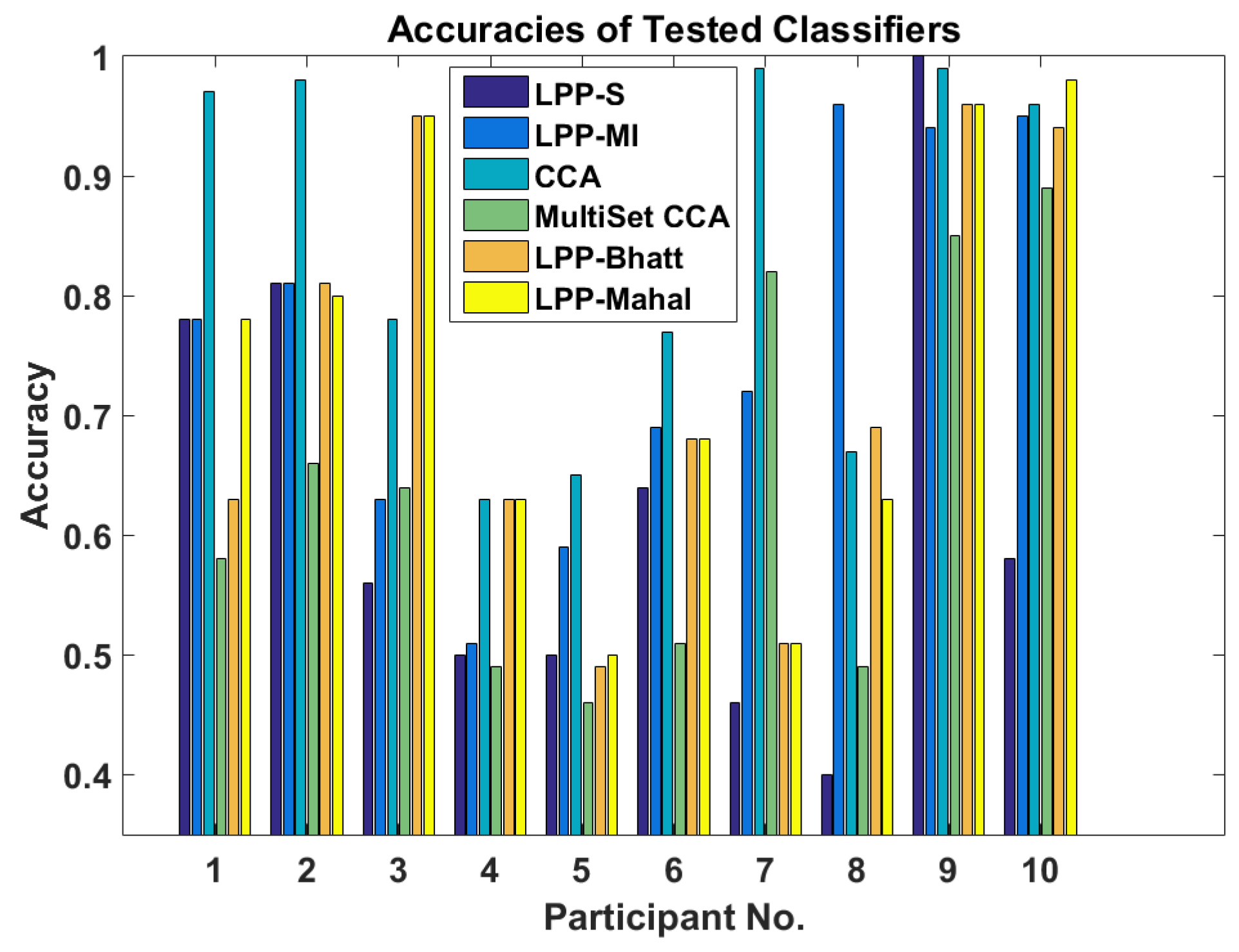
Figure 1 shows the accuracies for six different methods. The first one is a standard Learn++.NSE ensemble (LPP-S) while the second is for the Learn++.NSE ensemble augmented with mutual information (LPP-MI). This comparison exists to show if the mutual information calculation aids classification. The third method is standard CCA where the reference signals are sines and cosines with frequencies corresponding to the first two harmonics of the presentation stimuli. The fourth method is MultiSet CCA with reference signals learned from previous data sets corresponding to a particular user. This gives CCA a transfer learning component that makes the comparison fairer. The fifth and sixth methods utilize Learn++.NSE augmented with Bhattacharyya distance (LPP-Bhatt) and Mahalanobis distance (LPP-Mahal) instead of mutual information. These additional transfer learning methods serve to compare mutual information to statistical measures. We performed a non-parametric statistical test; namely, the Wilcoxon rank sum test with the significance level of 0.05. This test showed that across all participants, the methods compared here are not significantly different from each other (p = 0.1730). However, looking at Figure 1 more carefully, we observe that for participants 3, 4, 8, 9, and 10, the performance of the proposed transfer learning method is comparable to or better than CCA.

LPP-MI saw a large increase in accuracy over LPP-S and a small increase over other LPP ensembles. However, CCA performed best across all users. On the other hand, MultiSet CCA performed worse than both LPP-MI and CCA when using data sets from previous sessions to form the reference signal.

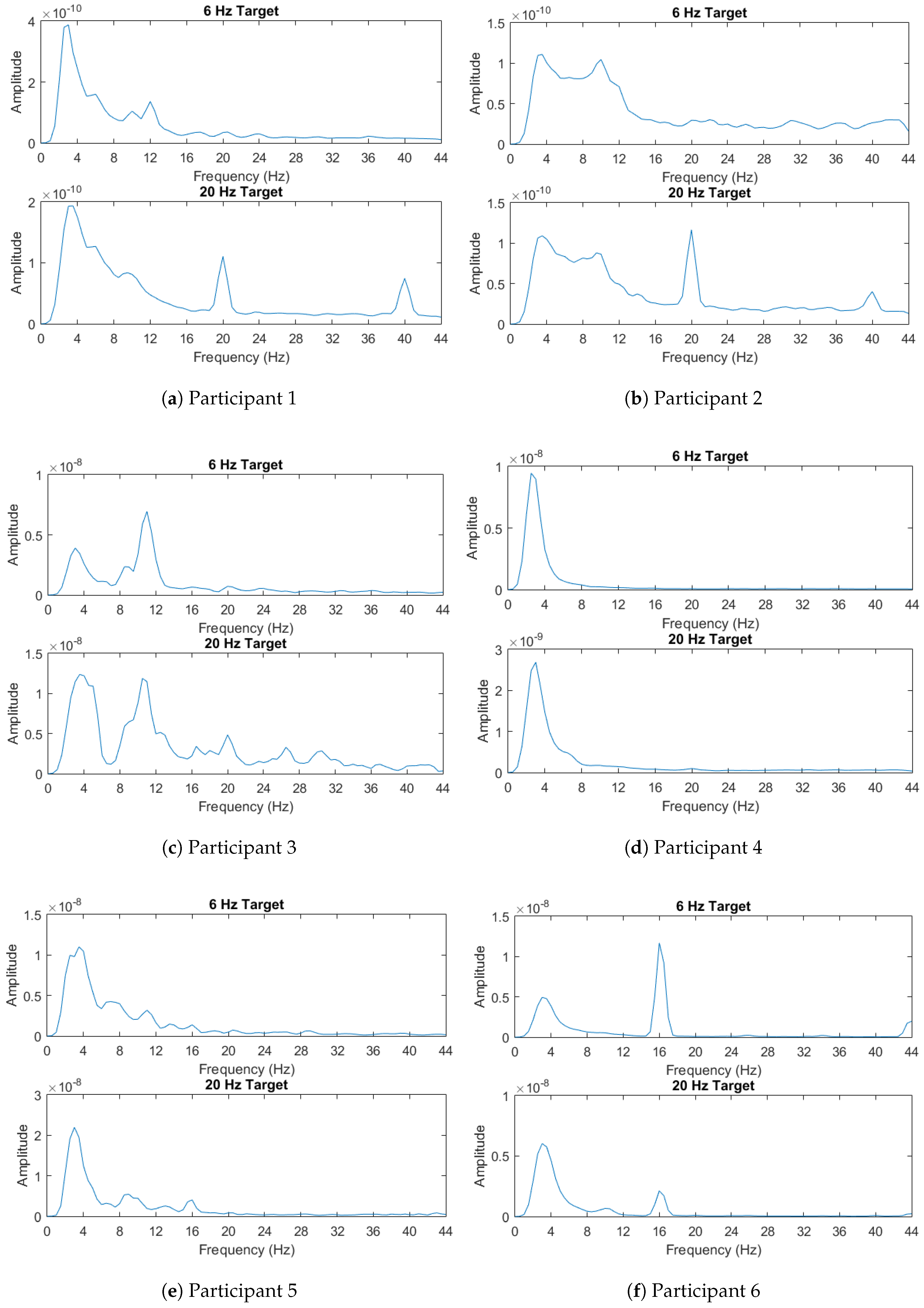
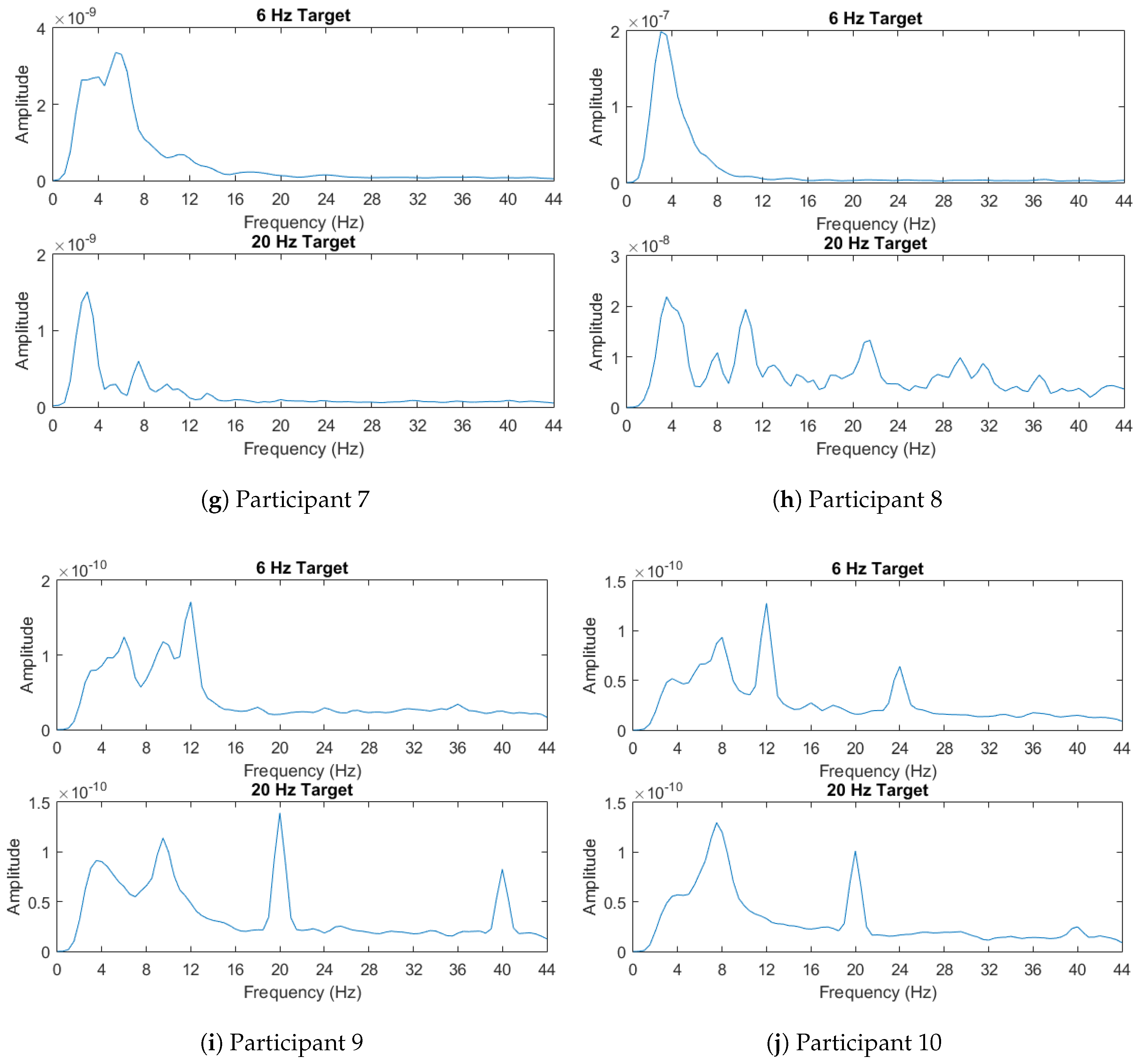
Participant 8 should be noted where LPP-MI performed best by a wide margin. This participant had a much stronger response to the 6 Hz stimulus than the 20 Hz one as shown in Figure 2. A linear discriminant analysis (LDA) classifier was also attempted on this participant with an accuracy of 74 percent.

Participant 3 also show increased performance over CCA using Learn++.NSE with Bhattacharyya or Mahalanobis distance as the similarity measure. Participants 4, 9, and 10 all saw comparable performance between at least one of the LPP variants and CCA. Additionally, participant 5 showed poor performance with CCA, but CCA still outperformed all other methods.

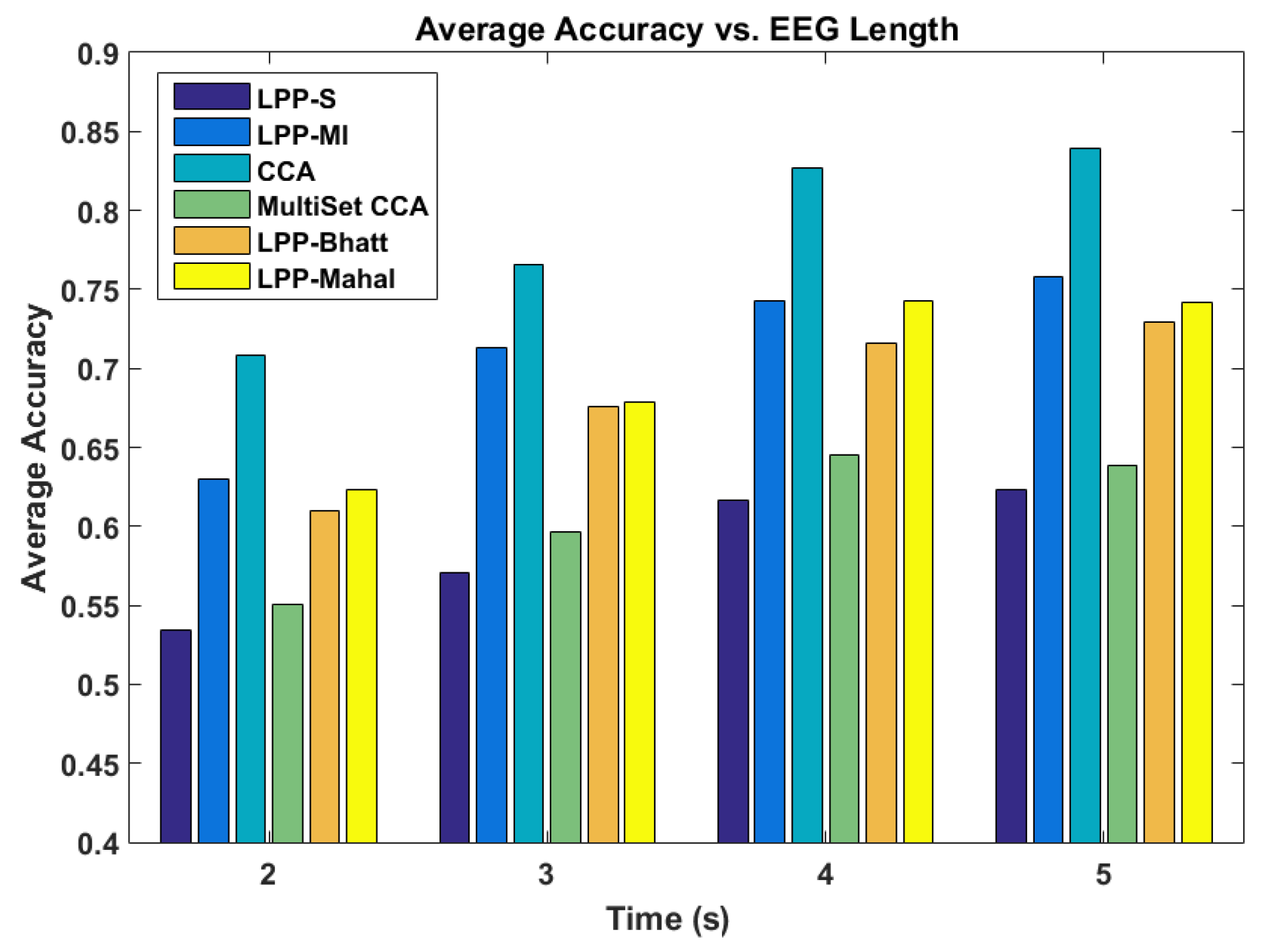
The performance of the various systems was also assessed as a function of the length of the EEG segment used for classification. The results are shown in Figure 3. Changing the length of the EEG segments did not change the performance of the various methods relative to each other. Regardless of EEG segment length, CCA performed the best when averaging the results across all the system users. LPP-MI performed best of the LPP ensembles, with Mahalanobis and Bhattacharya distances providing similar but slightly worse performance. However, all methods saw an increase in accuracy as the length of the EEG increased, with diminishing returns as the length approached 5 s.

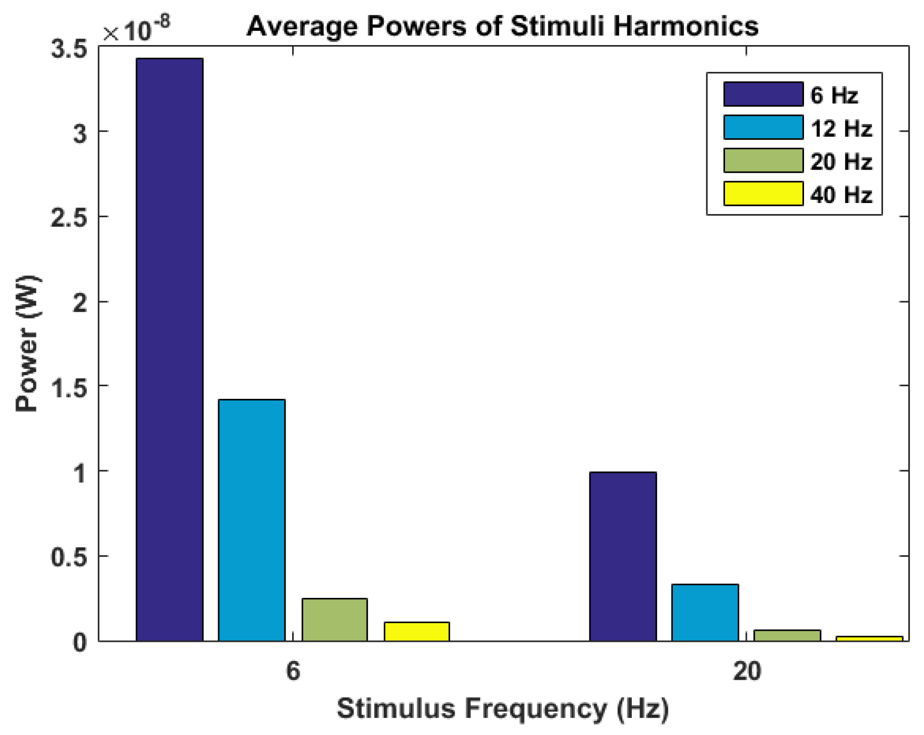
Lastly, the power spectral densities averaged across all trials for the target are shown in Figure 4. For each participant, in this figure, we illustrate the power spectral densities computed using the EEG recorded in response to stimuli flickering with two different frequencies, 6 and 20 Hz. As described in Section 4.4, the power spectral densities are calculated using Welch’s method. For some participants such as 9 and 10, the spikes in the power spectral densities are readily apparent and they provide features that can enable identification of the flickering stimulus. Others such as participants 4 and 8 show more indistinguishable responses to two different stimuli flickering with different frequencies. This might yield insight into the relatively poor performances of different classifiers for these specific participants.

3. Discussion

The participant pool in this study consisted of healthy users who were able to fully divert their covert attention toward the targeted checkerboards. For this reason, the relative success of CCA over other techniques is expected given its current position as state-of-the-art for SSVEP BCI systems.

However, participant 8’s unusual responses to the two stimuli frequencies makes for a good test case of someone who may not have full control of their covert attention. In this case, CCA would fail since the first target’s frequencies would always be chosen. This requires machine learning techniques and transfer learning if incorporating support for multiple data sets. Mutual information and Learn++.NSE allows for this transfer learning. In this case, the algorithm used a combination of participant 8’s own data and two other data sets to achieve its accuracy.

Participant 3’s performance with the LPP-Bhatt and LPP-Mahal ensembles also surpassed the CCA performance. Participant 3’s EEG signal was found to have more noise in frequency bands not of interest. Some noise was likely in the frequencies of interest as well. This may indicate that noisy signals may perform better with Learn++.NSE with similarity measures than CCA.

In the case of participants 4, 9, and 10, other LPP variants provided similar or better performance to CCA. Participant 4’s power spectral densities were very difficult to discern from each other, while participants 9 and 10 displayed expected power spectral densities. This may indicate that various LPP ensembles can match CCA both for abnormal or normal EEG on a case by case basis.

Participant 5 showed poor performance across all the classification schemes, but CCA still performed best in this case. In Participant 5’s power spectral density, the response to the 20 Hz stimulus was weak, leaving of the observed differences in the 6 Hz band. This would explain the poor performance across all the methods. Given that the power spectral density does not resemble that of another user, it is also not surprising that the LPP ensembles also performed poorly.

Multiset CCA appears to perform worse than CCA in every case. This may be due to the nonstationarity between data sets reducing the effectiveness of the generated reference signal.

As we illustrate with an experimental study, we identified certain users that could benefit from the transfer learning method proposed in this manuscript. Especially, we observed that for some users (3, 4, 8, 9, and 10), the proposed method may achieve comparable or higher accuracies than CCA.

The results of the investigation show that further effort is needed to reduce calibration requirements for non ideal usage cases. This includes users without full gaze control or unusual SSVEP responses. Similarity measures such as mutual information and ensemble learning are possible venues to explore toward this end. Further modifications are possible. For example, using the similarity measures as a score within the Learn++.NSE algorithm may improve results.

Additional investigation into users with unexpected EEG responses should be done in order to make statistical conclusions about the performance of the Learn++.NSE ensembles relative to CCA. With ten participants and only a subset of those with abnormal EEG spectra, results had to be compared on a case by case basis and it is what we illustrated in this manuscript.

There may be a way to combine the Learn++.NSE algorithm with CCA techniques in order to give better user transferability with CCA. This could be achieved by saving the CCA template signals for each user and adding them as members to the Learn++.NSE ensemble. The voting weights could then be determined as in typical Learn++.NSE applications. This may be one future direction in which transfer learning could be applied to CCA.

4. Materials and Methods

4.1. Learn++.NSE

Learn++.NSE was chosen as the ensemble learning algorithm due to its ability to assign useful weights for ensembles of any size while keeping computational complexity low. The details of this algorithm are summarized in Algorithm 1 [15].

First, define an ensemble hypothesis for a given data point at a discrete time t as $H^t\left(x\right)$. Voting weights $V^t$ for each of the $k^t$ ensemble members must be found.

$$V^t=[V_1^t,V_2^t,\cdots ,V_{k^t}^t]$$

(1)

Each of the $k^t$ individual member hypotheses $h_{k^t}^t\left(x\right)$ will generate up to c candidate decisions for the entire ensemble. The final ensemble hypothesis $H^t\left(x\right)$ is chosen such that:

$$H^t\left(x\right)=arg\underset{c}{max}(\sum _{i=1}^{k^t}(h_i^t\left(x\right)==c)\ast V_i^t)$$

(2)

Next, a data weight distribution $w^t$ for the incoming training data set is defined. The distribution is initialized uniformly, so $w^t\left(i\right)=\frac{1}{m^t}$, where $m^t$ is the amount of training data points in newly available data set $D^t$.

First, the ensemble error rate, $E^t$, is assessed on the data set $D^t$. This is done using the previous ensemble hypothesis $H^{t-1}\left(x\right)$ from $k^{t-1}$ member classifiers on each data point x in $D^t$. Each of the i data points in $D^t$ is assigned a new weight $w^t\left(i\right)$ by multiplying its current weight by the ensemble error rate $E^t$ if the data point was classified correctly by the ensemble. Since $E^t\le 1$, correctly classified points will always have a lower weight in the distribution. These steps are represented by Steps 4 and 5 in Algorithm 1.

Algorithm 1: Outline of the Learn++.NSE algorithm.

Data: Data set $D^t$ of length $m^t$

A designated base classifier algorithm

Real valued (a,b) sigmoid parameters

Ensemble hypotheses $H^t\left(x_i^t\right)={\hat{y}}_i^t$ with size $k^t$

Result: Trained ensemble $H^t$

for t = 1, 2, 3, ... do

end

Learn++.NSE handles nonstationarities by adding a new hypothesis $h_{k^t}^t\left(x\right)$ on the most recent training data set $D^t$ and by calculating voting weights $V^t$ of the resulting ensemble. The voting weights are found by evaluating the individual classifier error rate ${ϵ}_k^t$ for each of the $k^t$ classifiers as shown by Step 5. These error rates are also affected by the data weight distribution $D^t$. Note that the age of the ensemble members is not directly taken into account.

A sigmoidal error weighting scheme is included in Step 7 to prevent overfitting to the data [15]. The sigmoid curve weight before normalization, $\omega \left(t\right)$, is defined by:

$${\omega }_k^t=\frac{1}{1+e^{-a(t-k-b)}}$$

(12)

In this formula, k is the classifier position within the ensemble. The quantity $t-k$ is the time difference between the current time and the classifier creation time. Two parameters a and b are also introduced. These control the slope and horizontal offset respectively. These hyperparameters need to be tuned according to the data [16]. This was accomplished using a grid search in the hyperparameter space using ten-fold cross validation for testing, with nine-fold internal cross validation for every point in the hyperparameter space.

The final classifier voting weight of classifier k, $V_k^t$, is based on a combination of the errors from the current and past data sets. The weighted error rate ${\overline{\beta }}_k^t$ is calculated based on the procedures shown in Step 7.

The final voting weights for the k-th classifier, are obtained by taking the log reciprocal of the ${\overline{\beta }}_k^t$ [2].

4.2. Incorporating Mutual Information

Mutual information is a measure of how much information one random variable provides about another. In this experiment, mutual information was used as a method for finding which previously collected data sets best represented the incoming data set. In general, the mutual information between vector random variables X and Y is defined as [17]:

$${\int }_X{\int }_{Y}p(X,Y)log(\frac{p(X,Y)}{p\left(X\right)p\left(Y\right)})dYdX$$

(13)

Applying a Gaussian distribution assumption, the mutual information between X and Y of equal dimension with covariance matrices $C_X$ and $C_Y$ respectively can be calculated as:

$$I(X:Y)=\frac{1}{2}log(\frac{det\left(C_X\right)det\left(C_Y\right)}{det\left(C\right)})$$

(14)

The covariance matrix C is the full covariance matrix obtained by concatenating X and Y. If a data set contains n vectors for each variable, then there are $n^2$ combinations that will yield their own unique estimates of C. Averaging these estimates will reduce the overall estimate variance of C.

The mutual information can be incorporated into Learn++.NSE by receiving a new training data set. From that data set, the true class labels can be used to calculate the posterior probability distributions for each class. The total mutual information between every pre-existing data set and the incoming data set is found. From there, the m highest ranking data sets are chosen for training in the Learn++.NSE framework where the lowest ranking data set is introduced first, thereby making it the oldest classifier in the ensemble.

4.3. Statistical Measurement Comparisons to Mutual Information

There are other methods with which the similarity of distributions can be assessed. Two of these are considered for this paper. Mahalanobis distance allows the distance of a vector from a distribution given its mean vector μ and covariance matrix C [18]:

$$M\left(\overrightarrow{x}\right)=\sqrt{{(\overrightarrow{x}-\overrightarrow{\mu })}^T{C}^{-1}(\overrightarrow{x}-\overrightarrow{\mu })}$$

(15)

Bhattacharyya distance is similar in its goals but instead measures the distance between two distributions. For two distributions P and Q, the Bhattacharya distance is [18]:

$$B(P,Q)=\int \sqrt{P\left(\overrightarrow{x}\right)Q\left(\overrightarrow{x}\right)}d\overrightarrow{x}$$

(16)

Applying the same normality assumptions as the mutual information, the Bhattacharyya distance can be calculated from the means and covariances of P and Q:

$$B(P,Q)=\frac{1}{8}{(\overrightarrow{{\mu }_1}-\overrightarrow{{\mu }_2})}^T{C}^{-1}(\overrightarrow{{\mu }_1}-\overrightarrow{{\mu }_2})+\frac{1}{2}ln(\frac{det\frac{C_1+C_2}{2}}{\sqrt{det\left(C_1\right)det\left(C_2\right)}})$$

(17)

These distance metrics were used in the same way as mutual information to populate the ensemble except that data sets with minimal distance were chosen whereas maximum mutual information was used previously. This comparison exists to check if an information theoretic or statistical approach provides any differences in performance in the collected data sets.

4.4. Experimental Procedures

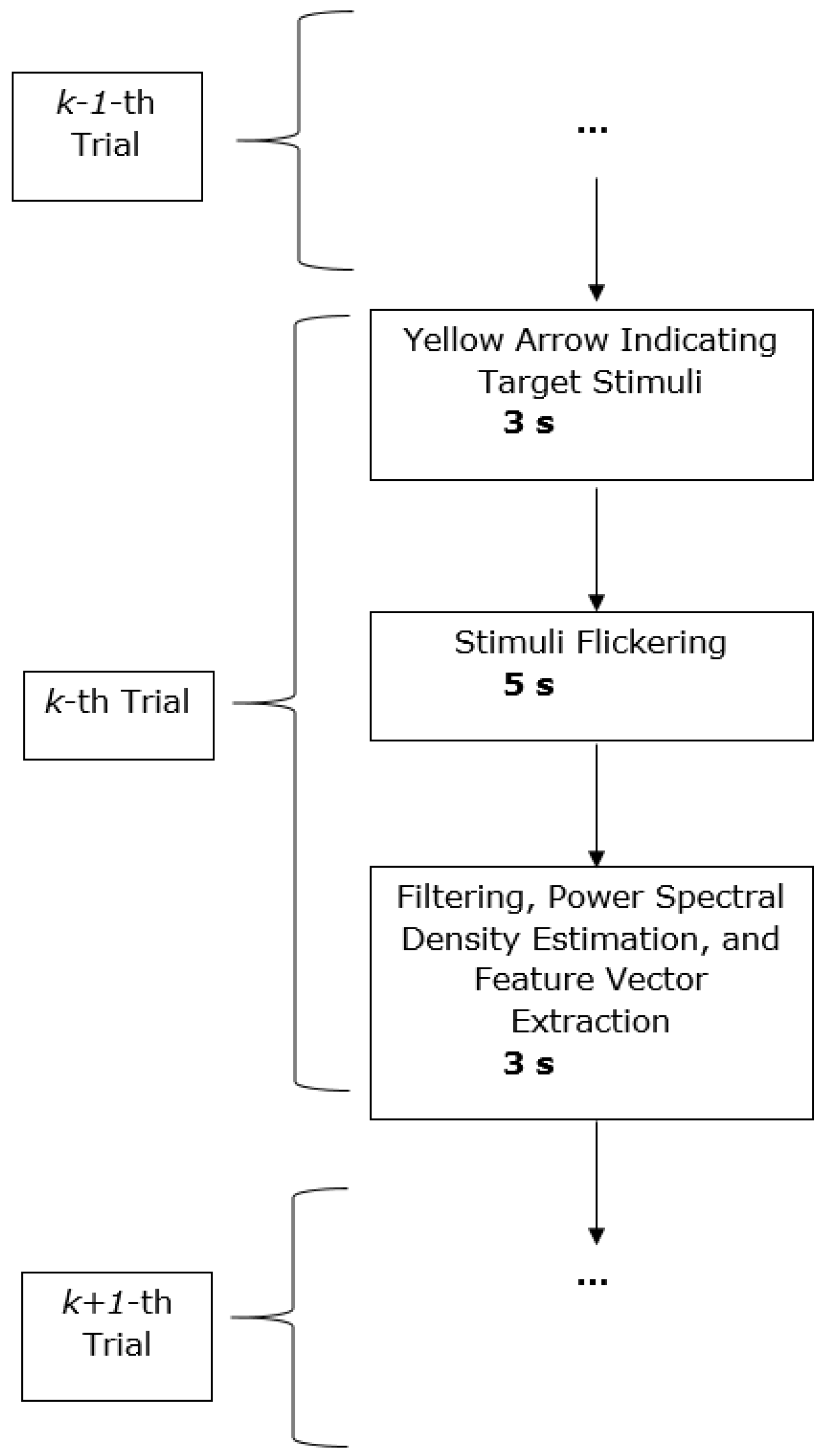
System Description: We developed an SSVEP-based BCI for binary selection that employed two flickering checkerboards at 6 and 20 Hz. The system was realized on a Lenovo ThinkPad laptop running 64-bit Windows 7. MATLAB 2015a was used for data acquisition, signal processing, feature extraction and classification; and Psychtoolbox (a freely available toolbox for creating time-accurate stimuli for experiments) was used for presentation. A general flowchart for system operation is shown in Figure 5.

The system was connected to a g.Tec g.USBamp via USB for data acquisition (g.USBamp—highest accuracy EEG amplifier, g.tec, Scheidlberg, Austria). The amplifier was connected to a g.gammaBox which was directly connected to the electrodes. Single channel EEG was used over the visual cortex (occidental zero on the 10–20 system) with a butterfly electrode. A ground electrode was placed over the forehead (frontal parietal zero on the 10–20 system). A reference electrode was clipped to the earlobe. A parallel port cable was also used to output digital values to the amplifier depending on the system’s current state. This digital value was sampled alongside the EEG data to easily separate the EEG data of interest.

Participant Description and Experimental Procedures: Ten healthy participants (eight males and two females) were enrolled in this study according to the University of Pittsburgh IRB No. PRO15060140. All participants were required to be at least 18 years of age and have no history of epilepsy. Ages ranged from 20 to 26 with an average age of 22.1 years and a standard deviation of 1.79 years.

All participants were asked to direct their covert attention randomly at one of the two checkerboards at the start of every trial. Each trial consisted of flickering of the checkerboards for 5 s. In one usage session, one hundred trials were presented. There were three usage sessions. In all sessions, a calibration phase was taken to collect training data. On the final session, a test phase of equal length was used to collect testing data where the ensemble would be evaluated.

Signal Processing and Feature Extraction: The EEG data was sampled at 256 Hz and filtered using a 150th order constrained least squares FIR filter from 2 to 45 Hz [19]. A power spectral density estimate was obtained using Welch’s method using windows of two seconds with 50 percent window overlap [20]. Features were made using the first two harmonics of the stimuli frequencies to obtain a four dimensional feature vector.

Classification: A linear discriminant classifier was used in the Learn++.NSE ensemble to reduce computational complexity. For each participant, ensembles were formed using groups of three individual classifiers. Two groups of ensembles were generated. The first group consisted of the mutual information-based Learn++.NSE ensembles (designated LPP-MI). Here, the mutual information between the latest data set recorded from a certain participant and all other data sets from all the participants were computed. The latest data set for the current user and the two data sets with the most mutual information were used for the training of LPP-MI for that specific participant. Specifically, the data sets were added to the Learn ++ algorithm in the following order: (1) the set with second most mutual information; (2) the set with most mutual information; and (3) most recent data set for that user. The second group contained the standard Learn++.NSE ensembles (denoted as LPP-S). For each participant, LPP-S was formed using the three training data sets corresponding to that specific participant. Choosing an ensemble size of three provided a reasonable compromise between practical computability and having multiple classifiers. An LDA classifier was also trained for each participant on their last session’s calibration phase in order to compare performance under typical calibration procedures. The three classifiers were then compared by examining their accuracies over the test data which was not used for training.