Misalignment Fault Diagnosis of DFWT Based on IEMD Energy Entropy and PSO-SVM

Abstract

Misalignment is an important cause for the early failure of large doubly-fed wind turbines (DFWT). For the non-stationary characteristics of the signals in the transmission system of DFWT and the reality that it is difficult to obtain a large number of fault samples, Solidworks and Adams are used to simulate the different operating conditions of the transmission system of the DFWT to obtain the corresponding characteristic signals. Improved empirical mode decomposition (IEMD), which improves the end effects of empirical mode decomposition (EMD) is used to decompose the signals to get intrinsic mode function (IMF), and the IEMD energy entropy reflecting the working state are extracted as the inputs of the support vector machine (SVM). Particle swarm optimization (PSO) is used to optimize the parameters of SVM to improve the classification performance. The results show that the proposed method can effectively and accurately identify the types of misalignment of the DFWT.

1. Introduction

The development of the wind energy is very rapid with growing concerns about the energy and environmental problems nowadays. The global cumulative installed capacity reached 432,419 MW at a compound growth rate of 17% per year [1]. Wind farms mainly use the large capacity variable speed constant frequency (VSCF) doubly-fed wind turbines (DFWT) as the main models [2]. Its structure mainly includes the rotor, shaft, gearbox, the doubly-fed induction generator (DFIG), the converter, etc. Because of the long transfer chain of DFWT and the installation in the cabin at high altitude of tens of meters, or even hundreds of meters, precise alignment is rather difficult; on the other hand, due to the fluctuation of wind speed, start-stop of the units frequently happened. As time goes on, there will be a shift or deformation in some components, causing the misalignment between the generator and the gearbox [3]. When misalignment happens, gearbox high-speed shaft and generator bearings will produce heavy dynamic load, which will not only increase axial and radial vibration, but also cause the bearing oil leakage, high temperature of bearing and attachment bolts and fastening bolts loosening. The accumulation of eccentric error even causes damage to bearings of the high-speed end and generator. Because misalignment is an important cause of early failure of large DFWT and may cause damage to two core parts including the gearbox and generator, it is necessary to study the misalignment fault diagnosis methods to ensure longstanding and stable running of the DFWT.

At present, there are many methods used in the wind turbines fault diagnosis. For example, the back propagation (BP) neural network based on the fruit flies algorithm optimization was used by Qi Liwan in fault diagnosis for the wind turbine gearbox [4]; a fault diagnosis method based on learning vector quantization (LVQ) neural network was proposed by Ding at al. [5]; the fuzzy clustering analysis method was applied to the wind motor gearbox fault by Li [6]; the fault classification method based on the ART2 neural network and C-average clustering algorithm of wind turbine gearbox was used by Li et al. [7]; an expert system model for the fault diagnosis of a wind turbine cabin was established by Zhang [8]; a classification method based on support vector machine (SVM) was proposed by Liu et al. to classify the operating mode of wind turbines [9]; a wind turbine main shaft bearing fault diagnosis based on SVM was studied by Huang [10]; machine learning and data mining techniques organized in the framework of a general scheme that achieves fault diagnosis of wind turbines were studied by Precup et al. [11]; a hybrid dynamic classifier for drift-like fault diagnosis was applied to wind turbine converters by Toubakh [12]; a mixed Bayesian/Set-membership approach was used by Rosa et al. to solve the problem of fault detection and isolation of wind turbines [13]; the interval nonlinear parameter-varying (NLPV) parity equations were used by Blesa et al. to solve the problem of fault diagnosis of a wind farm [14]; and the interval observer approach and virtual actuators/sensors were applied by Blesa et al. in literature [15], where the problem of Fault Detection and Isolation (FDI) and Fault Tolerant Control (FTC) of wind turbines were addressed. Compared with other intelligent algorithms, SVM has many advantages in learning ability, generalization performance, small sample processing capacity and the nonlinear processing capacity. Therefore, in this paper, SVM is used in the misalignment fault diagnosis.

There are three types of misalignment: parallel misalignment, angle misalignment and the comprehensive misalignment [16]. Due to the short running time of large DFWT in China, the data of misalignment available for diagnostic studies are lacking. Thus, a 3D model was established by Solidworks (Solidworks 2014, version SP0) for a 1.5 MW wind turbine in this paper, and the model is then imported into Adams (Adams 2013, version 2013.1), where the normal working and the misalignment of the system are simulated. The vibration signals (angular acceleration) of the gearbox high-speed shaft are obtained for analysis. The methods for extracting fault features from vibration signals mainly include traditional and modern signal processing methods [17]. The traditional signal processing methods include time domain analysis and frequency domain analysis. Signal stability hypothesis is the basis of the traditional time domain or frequency domain analysis. However, the vibration signals of DFWT usually have the characteristics of being nonlinear and non-stationary. Therefore, the modern signal processing methods should be used to analyze them. Many scholars have done a lot of work in this area. For example, wavelet decomposition was used by Zhang o process the vibration signals of gearbox in DFWT [18]; while wavelet packet was used by Wang [19], a method of multi resolution empirical mode decomposition (EMD) combined with the average in frequency domain was proposed by Ju et al. to extract gear fault frequency [20]; EMD and the envelope spectrum of the intrinsic mode function (IMF) was used by Zheng et al. to identify the fault types of rolling bearing [21] and so on. The advantages and shortcomings of modern signal processing methods now commonly used are summarized in

Table 1. Comparison of various modern signal processing methods.

Methods	Advantages	Shortcomings
Short Time Fourier Transform	Easy to implement; avoiding the cross-term interference in the high-order non-stationary analysis [22].	High redundancy; limited time-frequency aggregation; lacking of self adaptability [23].
Wiger-Ville	High time-frequency resolution; concentration of energy; having time-frequency edge characteristics [24].	Energy density is not guaranteed to be non-negative in all time and frequency ranges; a serious cross-term interference [25].
Wavelet Transform	Localized in time domain; multi resolution; adjustable analysis precision [26].	Leaking of energy; lacking of self adaptability [27].
Wavelet Packet Transform	Decomposing the low frequency portion while carrying out a more detailed decomposition to high frequency portion of the signal; no redundancy and no omissions [28].	Wavelet packet energy and time-frequency information are not intuitive [29].
Blind Source Separation	Identifying the original signal directly according to the observation information, solving the problem that the traditional methods can not solve [30,31].	Difficulty in identifying the unknown or dynamic change signal source [30,31].
High-order Statistics Analysis	Ability of automatically suppress the influence of Gaussian colored noise and some non-Gaussian colored noise; high-order cyclic statistics can automatically suppress any stationary (Gaussian and non-Gaussian) noise [30].	Complicated and no clear physical meaning [30].
EMD	Suitable for nonlinear and non-stationary signal analysis; high signal-to-noise ratio; self adaptation; orthogonality and completeness; high efficiency [32,33].	End effect problem; mode mixing problem and the limitations of decomposition [34].

.

Among these commonly used processing techniques summarized in Table 1, EMD proposed by Hibert–Huang is a signal processing technique to decompose a data set into several IMFs by a sifting process, reducing the coupling between the signal characteristic information. Using the EMD method, the feature information of the original data can be grasped accurately and effectively, which is conducive to mining deep feature [35]. However, there will be divergent phenomenon at both ends of the date when using the EMD method, which may result in the entire data sequence gradually being contaminated and the decomposition effect becoming severely distorted [36,37,38,39]. To solve this, a mirror extension algorithm is used to improve the EMD in this paper. After the vibration signals of DFWT processed by the IEMD, the energy entropy of the IMF are calculated and taken as the inputs of SVM. Meanwhile, PSO is used to optimize the parameters of SVM to get better classification performance. The results show that the proposed method can effectively identify the different misalignment types.

2. The Related Theories

2.1. The Improved EMD

The basic idea of EMD is to decompose a complex non-stationary signal into a finite number of IMF, and the IMF must satisfy the following:

• The amount of extreme values and passing zeros of the function must be equal to or differ by one at most;
• The average value of the upper envelope formed by the local maximum points and the lower envelope formed by the local minimum points of the function is zero.

The specific steps of decomposing the original signal $x(t)$ by EMD are as follows:

(1)

Find out all the maximum points and the minimum points of the original signal firstly. Then, fit the upper envelope $e_{upp}(t)$ and the lower envelope $e_{low}(t)$ by the cubic spline interpolation. The average value $m_1(t)=\frac{e_{upp}(t)+e_{low}(t)}{2}$ can be obtained. Assume:

$$w_1(t)=x(t)-m_1(t).$$

(1)

(2)

Judge whether $w_1(t)$ meets the two conditions of IMF. If it is satisfied, then $w_1(t)$ is the first IMF component; if not, then take $w_1(t)$ as a new $x(t)$. Repeat step (1) until $w_{1k}(t)=w_{1(k-1)}(t)-m_{1k}(t)$ meets the two requirements.

(3)

After the first IMF component $c_1(t)$ is decomposed from the original signal $x(t)$, separate $c_1(t)$ from $x(t)$ to get the rest $r_1(t)$:

$$r_1(t)=x(t)-c_1(t).$$

(2)

Take $r_1(t)$ as the original data and repeat steps (1), (2) and (3). The second IMF component of the original signal can be then obtained. Repeat n times, and $r_1(t)$, $r_2(t)$,…, $r_N(t)$ can be obtained. The process will last until the remainder $r_N(t)$ becomes a monotonic function.

Finally, $x(t)$ can be expressed as follows:

$$x(t)={\displaystyle \sum _1^N{c}_i(t)}+r_N(t).$$

(3)

The IMF components contain different frequency band elements of the original signal $x(t)$, while the remaining part $r_N(t)$ represents the central tendency of $x(t)$.

According to the maximum values and minimum values provided by the original signal, cubic spline interpolation is performed to obtain the upper and lower envelope in the EMD processing. However, the two end points of the signal may not be extreme value points, which will produce the fitting error. The error will gradually spread to the inside signal with the decomposition process, causing the waveform of IMF component to become seriously distorted. This is called the end effects of the EMD. In order to maintain the authenticity of the data, the mirror extending method is used to improve the EMD in this paper.

The mirror extending method is based on the characteristics of mirror symmetry mapping. To minimize the side effect, the mirror is placed in the position that ensures that the signal has symmetrical extreme values. The specific steps are:

(1)

To draw the curves at both ends and mark the corresponding extreme values (the maximum and minimum);

(2)

To decide the position of the mirror according to the distribution characteristics of the curves, and make the signal in the mirror and the original signal connected end-to-end to form a closed loop;

(3)

To get the new signal with the length of two times the original data.

By extension, the upper and lower envelope obtained by fitting are completely determined by the internal data, and the end effects are solved in essence.

2.2. The Principles of SVM

SVM was proposed by Vapnik in 1995, which takes the training error as the constraint condition of the optimization problem and minimizes the confidence range as the objective of optimization. SVM is a kind of learning method based on structuring risk minimization principle, with better promotion ability than other traditional methods [40]. Since the solving process of SVM is finally transformed into a quadratic programming resolving, its solution is the only optimal one. SVM shows many unique advantages in solving nonlinear and high-dimensional pattern recognition problems [41,42,43]. The principle of SVM can be briefly described as giving training samples $(x_1,y_1)$, $(x_2,y_2)$, …, $(x_l,y_l)$, where $x_i\in R^n$, $y_i\in \{1,-1\}$, and $l$ is the number of training samples. They can be separated by a hyper plane, and the hyper plane can be expressed as follows:

$$\omega x+b=0,$$

(4)

where $\omega$ and $b$, respectively, represent the normal vector and the constant term. When $\omega$ and $b$ are the best, it means the optimal hyper plane has been found, which makes the distance between the positive and negative samples the largest.

For linearly inseparable problems, the samples can be mapped to the hyper plane by the kernel function $K(x_i,y_j)$ to realize linear separability. Its objective function is as follows:

$$\begin{gathered} W(a)={\displaystyle \sum _{i=1}^l{a}_i}-\frac{1}{2}{\displaystyle \sum _{i=1}^l{\displaystyle \sum _{j=1}^l{a}_i{a}_j{y}_i{y}_{j}K(x_i,x_j)}}, \\ s.t.{\displaystyle \sum _{i=1}^l{a}_i{y}_i}=0,0\le a_i\le C \end{gathered}$$

(5)

where $a_i$ is the Lagrange operator; $C$ is the punishment factor, and its basic function is to control the penalty of the wrong samples; $K(x_i,x_j)$ is the kernel function, and its basic function is to transform the vectors of low-dimensional to the inner product in the high-dimensional.

The kernel functions used in SVM are mainly linear kernel function, polynomial kernel function, radial basis kernel function and sigmoid kernel function. For the selection of kernel function, there is no definite criterion. Many studies and experiments show that the radial basis function (RBF) is a better choice when there is not enough prior knowledge [44]. In this paper, the RBF is used as the kernel function. The function is as follows:

$$K(x_i,x_j)=\exp (-g{\Vert x_i-x_j\Vert }^2),g>0,$$

(6)

where $g$ is the kernel parameter.

After determining the type of kernel function, the penalty parameter $C$ and the RBF parameter $g$ should be decided. Parameter $C$ determines the training error and the generalization ability of the classifier; parameter $g$ affects the distribution form of the samples in the feature space. The selection of them is very important for the performance of the classifier. The traditional grid search is a way to find the optimal parameters, but the search result may not be necessarily good. Thus, in this paper, PSO is used to select the parameters of $C$ and $g$ to improve the classification performance.

2.3. Particle Swarm Optimization

PSO is a kind of swarm intelligence optimization algorithm besides the ant colony algorithm and the fish swarm algorithm, which was first proposed by Kennedy and Eberhart in 1995. PSO is used to initialize a group of particles in the solution space, and each particle represents a potential optimal solution to the optimization problem. The characteristics of the particles are represented by three indexes of position, velocity and fitness value. Fitness value can be calculated by the fitness function, and the size of the value represents the goodness and badness of the particle. The particles’ location are updated by tracking the individual extreme value and the population extreme value when they move in the solution space. The fitness value of each particle is calculated when it updates its location. The principle can be briefly described as follows.

Supposing in a $D$-dimensional search space, there is a population $X=(X_1,X_2,\dots ,X_n)$, consisting of $n$ particles. The i-th particle is represented as a D-dimensional vector of $X_i=[x_{i1},x_{i2},\dots ,x_{iD}]$, which represents the position of the i-th particle in the D-dimensional search space, and it also represents a potential solution to the problem. According to the objective function, the fitness value of each particle's position $X_i$ can be calculated. If the velocity of the i-th particle is $V_i=[V_{i1},V_{i2},\dots ,V_{iD}]$, the individual extremum is $P_i=[P_{i1},P_{i2},\dots ,P_{iD}]$, the population extremum is $P_g=[P_{g1},P_{g2},\dots ,P_{gD}]$, and then the velocity and position of the particle are updated according to the following equations:

$$V_{id}^{k+1}=V_{id}^k+c_1{r}_1(P_{id}^k-X_{id}^k)+c_2{r}_2(P_{gd}^k-X_{id}^k),$$

(7)

$$X_{id}^{k+1}=X_{id}^k+V_{id}^{k+1},$$

(8)

where $d=1,2,\dots ,D$; $i=1,2,\dots ,n$; $k$ is the number of iterations; $c_1$ and $c_2$ are learning factors, which are non negative constants, making the particles learn from their own or other better particles to achieve the purpose of being close to the better position of itself or the whole group; $r_1$ and $r_2$ are random numbers distributed in [0, 1] to maintain the diversity of group. In order to prevent the blind search of particles, it is generally recommended to limit the position and velocity to a certain range of $[-X_{\max },X_{\max }]$ and $[-V_{\max },V_{\max }]$.

3. Acquisition of Samples for Diagnosis

A 1.5 MW wind turbine system in a certain factory is studied in this paper. Gearbox, coupling, generator, etc., are modeling and assembling by SolidWorks firstly. Secondly, the models are saved in SolidWorks as Parasolid(.x_t) format. Then, they are imported into Adams. According to the actual status of the wind turbine system, material definition, motion constraints, drive and contact force for components and parts are added. In this paper, four states of normal working condition, parallel misalignment, angle misalignment and the comprehensive misalignment are studied, respectively. The models have been verified before the vibration signals are extracted from the gearbox high-speed shaft.

3.1. Verification of the Models

3.1.1. Normal Working State

At normal working state, the model is verified by the speed of the gearbox, generator shaft and the meshing frequency. The comparison of theoretical results and simulation results are listed in

Table 2. Comparison of theoretical results and simulation results at a normal working state.

Items	Simulation Rotational Speed (°/s)	Theoretical Rotational Speed (°/s)	Relative Error	Simulation Fundamental Frequency (Hz)	Theoretical Fundamental Frequency (Hz)	Relative Error
Low-speed solar gear	520.97	517.46	0.68%	26.22	26.39	0.64%
Medium-speed solar gear	2911.33	2918.47	0.24%	166.54	166.73	0.11%
High-speed pinion	10528.61	10527.34	0.01%	818.28	818.79	0.06%
Shaft of generator	10520.68	10527.34	0.06%	818.89	818.79	0.01%

.

It can be seen the relative error is very small by comparing the theoretical results with the simulation results in Table 2. This demonstrates that the model of normal working state is correct.

3.1.2. At Fault Conditions

The shaft radial force and axial force are used to test the validity of the failure models. In theory [45], the characteristics of misalignment can be summarized in

Table 3. The characteristics of misalignment.

Fault Type	Spectral Characteristics
Parallel misalignment	The fundamental frequency and frequency-doubled of power frequency of rotor system are relatively obvious; the radial vibration is more obvious than the axial vibration; the amplitude increases with the increment of the degree of the misalignment.
Angle misalignment	Angle misalignment produces large axial vibration, the vibration frequency is given priority to fundamental frequency; vibration amplitude increases with the increment of the degree of the misalignment.
Comprehensive misalignment	Contains the fault characteristics of parallel misalignment and angle misalignment.

.

The actual outputs of the failure models would be described below:

• Parallel Misalignment
  In Adams, the local coordinate system (Marker) can be created in the left half coupling mass center. In addition, the rotation axis of the revolute joint relative to the ground is arranged on a z-axis of the Marker global coordinate system. Then, the Marker global coordinate system is translated a certain distance along the y-axis to make the mechanism rotate. The deviation between the center of mass and the center of rotation can lead to the eccentric mass excitation to the mechanism; thus, the parallel misalignment of the rotor shaft of the generator in this distance can be simulated. Some results of the parallel misalignment are shown in

  Table 4. Some simulation results of the parallel misalignment.

  The Degree of Parallel Misalignment (mm)	Radial Force Times Frequency Amplitude (N)		Axial Force Times Frequency Amplitude (N)
  	Fundermental Frequence Amplitude	Frequency-Doubled Amplitude	Fundermental Frequence Amplitude	Frequency-Doubled Amplitude
  Normal condition	6657	687	1798	271
  1	8586	2058	2416	265
  2	20,936	16,841	6364	427
  3	36,515	18,411	11,114	405

  .
  From Table 4, it can be found that the fundamental frequency and the frequency-doubled of the radial force and axial force are obvious when parallel misalignment exists. With the increment of parallel misalignment, the amplitude increment of the fundamental frequency and frequency-doubled of the radial force is far bigger than axial force, that is, the radial vibration is the main. This is in accordance with the theoretical analysis shown in Table 3.
• Angle Misalignment
  The local coordinate system (marker) rotates a certain angle around the y-axis, and the z-axis of the local coordinate system is set up as the orientation of revolution joint, and then the corresponding angle misalignment can be simulated. Some results of the angle misalignment are shown in

  Table 5. Some simulation results of the angle misalignment.

  The Degree of Angle Misalignment (°)	Radial Force Times Frequency Amplitude (N)		Rxial Force Times Frequency Amplitude (N)
  	Fundermental Frequence Amplitude	Frequency-Doubled Amplitude	Fundermental Frequence Amplitude	Frequency-Doubled Amplitude
  Normal condition	6657	687	1798	271
  0.1	6864	716	3789	390
  0.2	7405	941	4314	399
  0.3	11,048	764	4408	384

  .
  From Table 5, it can be found the fundamental frequency of radial force and axial force are obvious when angle misalignment exists. With the increment of angle misalignment, the fundamental frequency amplitude is also increasing, but priority is given to the axial vibration. This accords with the theoretical analysis shown in Table 3.
• Comprehensive Misalignment
  Adding the parallel misalignment and angle misalignment in the local coordinate system (maker) of the left half coupling at the same time, comprehensive misalignment can be simulated. Some results of the comprehensive misalignment are shown in

  Table 6. Some simulation results of the comprehensive misalignment.

  The Degree of Comprehensive Misalignment	Radial Force Times Frequency Amplitude (N)		Axial Force Times Frequency Amplitude (N)
  	Fundermental Frequence Amplitude	Frequency-Doubled Amplitude	Fundermental Frequence Amplitude	Frequency-Doubled Amplitude
  Normal condition	6657	687	1798	271
  0.1°--1 mm	5519	4805	1577	888
  0.2°--2 mm	28,297	22,465	2280	1114
  0.3°--3 mm	39,164	19,214	4834	887

  .
  From Table 6, it can be seen that the radial vibration and axial vibration are obvious at the same time, as well as the fundamental frequency and the frequency doubling when the comprehensive misalignment happens. The simulation results verify the theoretical conclusion very well.
  Through validation, it can be concluded the simulation results accord with theoretical conclusions. This is effectively guaranteeing the validity of the extraction of vibration signals.

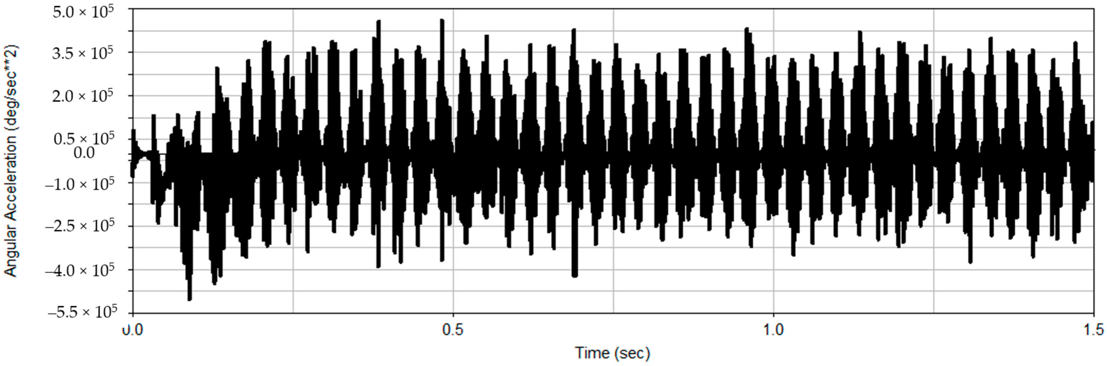
3.2. Acquisition of the Vibration Signals of the Gearbox High-Speed Shaft

In this paper, the vibration signals (angular acceleration) of the gearbox high-speed shaft are obtained for analysis.

According to the requirements of the selected unit, the allowance range of the parallel misalignment is 0–0.15 mm. The allowance range of the angle misalignment is 0°–0.05°. In these ranges, the wind turbine system runs normally. In this paper, the range of parallel misalignment simulated is 1–10 mm. The range of angle misalignment that simulated is 0.10°–10°. The samples used are simulated by the method described above from four cases of normal working conditions, parallel misalignment, angle misalignment and the comprehensive misalignment. Each kind of sample is 68, with a total of 272 samples.

4. Extracting IEMD Energy Entropy from the Vibration Signals

Entropy is a measure of the uncertainty degree of the information, including energy entropy, singular entropy, and the approximate entropy (they are generally referred to as the information entropy). Energy entropy has a very good effect on the extraction of non-stationary and nonlinear complex signal statistical characteristics [46]. Its definition is as follows:

Assuming

$$E_i={\displaystyle \int {\left|c_i(t)\right|}^2}dt={\displaystyle \sum _{k=1}^n\left|x_{ik}^2\right|},E={\displaystyle \sum _{i=1}^n{E}_i},p_i=\frac{E_i}{E},$$

(9)

where $i=1,2,3,\dots ,n$, $x_{ik}$ is the amplitude of each discrete point.

Then, the energy entropy is the following:

$$P_i=-{\displaystyle \sum _{i=1}^n{p}_i\lg p_i}.$$

(10)

When misalignment occurs in DFWT, the frequency of the vibration signal will change, and so will the energy distribution. Therefore, the energy entropy can be used to reflect the characteristics of vibration signals. In this paper, vibration signals are analyzed by the IEMD first, and then the energy entropy of the IMF components are calculated. Different numbers of the IMF may be obtained from different vibration signals, and the correlation coefficient method is used to determine the number of IMF components to be put into the SVM. The correlation coefficient method is to determine the correlation coefficient between the IMF information and the original signal [47]. Assuming that a non-stationary signal $x(t)$ can be decomposed into a finite mutually uncorrelated component $x_i(t)$, that is:

$$x(t)=x_1(t)+x_2(t)+\dots +x_N(t),$$

(11)

the correlation coefficient of each component and the original signal is calculated as:

$${\rho }_{x_{i}x}=\frac{{\displaystyle \sum _{t=0}^{\infty }{x}_i(t)x(t)}}{{[{\displaystyle \sum _{t=0}^{\infty }{x}_i^2(t)}{\displaystyle \sum _{t=0}^{\infty }{x}^2(t)}]}^2},i=1,2,\dots ,N,$$

(12)

and the larger the value of correlation coefficient, the greater the relevance, and vice versa.

For example, after processing the vibration signal, which is shown in Figure 1 by IEMD, the correlation coefficients of all IMF components are calculated as shown in

Table 7. Correlation coefficient of each IMF component and the original signal.

Object	IMF1	IMF2	IMF3	IMF4	IMF5	IMF6	IMF7
Correlation coefficient	0.6403	0.5440	0.3391	0.2374	0.1403	0.0903	0.0913
Object	IMF8	IMF9	IMF10	IMF11	IMF12	IMF13
Correlation coefficient	0.1086	0.0448	0.0332	0.0490	0.0579	0.0006

.

The contribution rate of the first eight IMF components in 13 IMFs reaches 92.23%. Thus, it can be concluded that the first eight IMFs contain the main information of the signals. Through a lot of experiments, it is known that the correlation between the first several IMF components and the original signal are relatively big. The contribution rates of the first eight IMFs are over 90%. Therefore, they are used to calculate the energy entropy to characterize the different states in this paper. The partial data of the first eight IEMD energy entropies of the vibration signals are shown in

Table 8. The partial data of the first eight IEMD energy entropies of vibration signals in different working conditions.

Fault Type	P1	P2	P3	P4	P5	P6	P7	P8
Normal condition	0.3109	0.3429	0.1709	0.0747	0.0476	0.072	0.097	0.0521
	0.3166	0.352	0.1553	0.0784	0.0477	0.0688	0.0575	0.0176
	0.3186	0.3498	0.1657	0.0814	0.0478	0.0452	0.069	0.0172
	0.3256	0.341	0.2031	0.0895	0.0564	0.037	0.0933	0.0148
	0.3302	0.3386	0.1669	0.0748	0.0574	0.0522	0.0788	0.0129
Parallel misalignment	0.1484	0.3676	0.3623	0.193	0.1201	0.0863	0.0477	0.1012
	0.1489	0.3669	0.3678	0.2267	0.0938	0.0481	0.028	0.1249
	0.1513	0.3678	0.3662	0.1839	0.1077	0.0665	0.0517	0.2216
	0.1558	0.3533	0.3675	0.2133	0.1479	0.0683	0.0637	0.1977
	0.1574	0.3601	0.3639	0.157	0.0807	0.062	0.2031	0.1429
Angle misalignment	0.2335	0.3067	0.2325	0.1467	0.0843	0.0763	0.1386	0.3648
	0.2361	0.3024	0.3679	0.289	0.1934	0.1157	0.1594	0.0478
	0.2423	0.3665	0.3417	0.2574	0.1862	0.0897	0.0395	0.0279
	0.2455	0.3476	0.3679	0.3096	0.1083	0.0873	0.0337	0.0536
	0.2487	0.3298	0.3134	0.2565	0.1254	0.0804	0.1309	0.3447
Comprehensive misalignment	0.1456	0.2285	0.2912	0.3322	0.2521	0.1672	0.2001	0.1162
	0.1061	0.2784	0.3393	0.2876	0.2762	0.0813	0.2059	0.1677
	0.1074	0.2581	0.3357	0.3582	0.1606	0.1101	0.1396	0.1396
	0.1082	0.2853	0.3271	0.3022	0.1685	0.1765	0.0751	0.1556
	0.111	0.3268	0.3654	0.2737	0.2681	0.0886	0.0773	0.1014

.

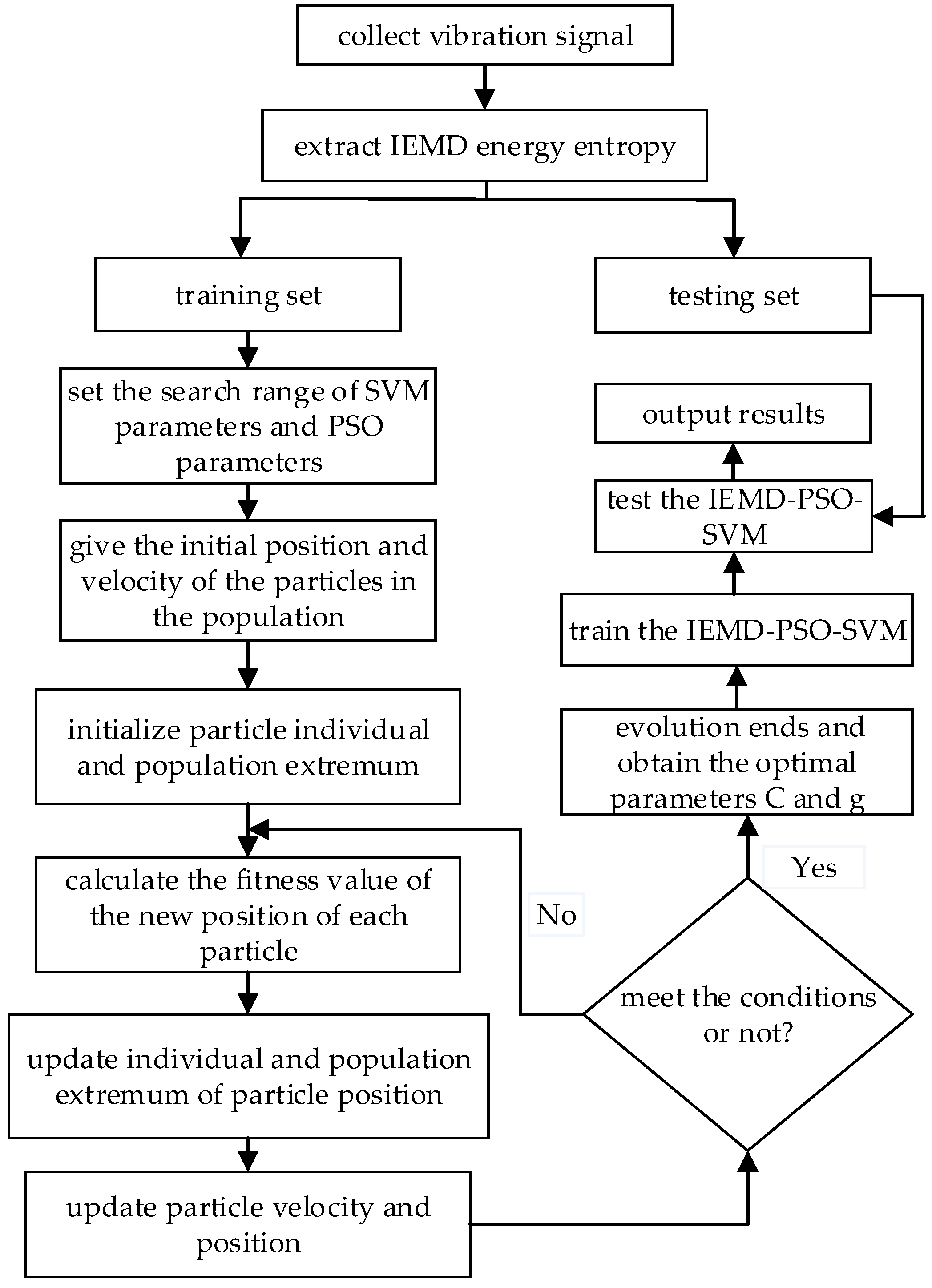
5. Fault Diagnosis Based on IEMD Energy Entropy and PSO-SVM

After extracting the IEMD energy entropy of the vibration signals, the samples were divided into two equal groups, one was the training set, containing 45 × 4 samples, and the other was the testing set, containing 23 × 4 samples. The training samples were used to obtain the optimized SVM classifier (3-fold cross validation). The PSO algorithm was used to optimize the penalty parameter $C$ and kernel parameter $g$ of SVM, and the whole fault diagnosis processing can be referred to as IEMD-PSO-SVM; the specific implementation is shown in Figure 2.

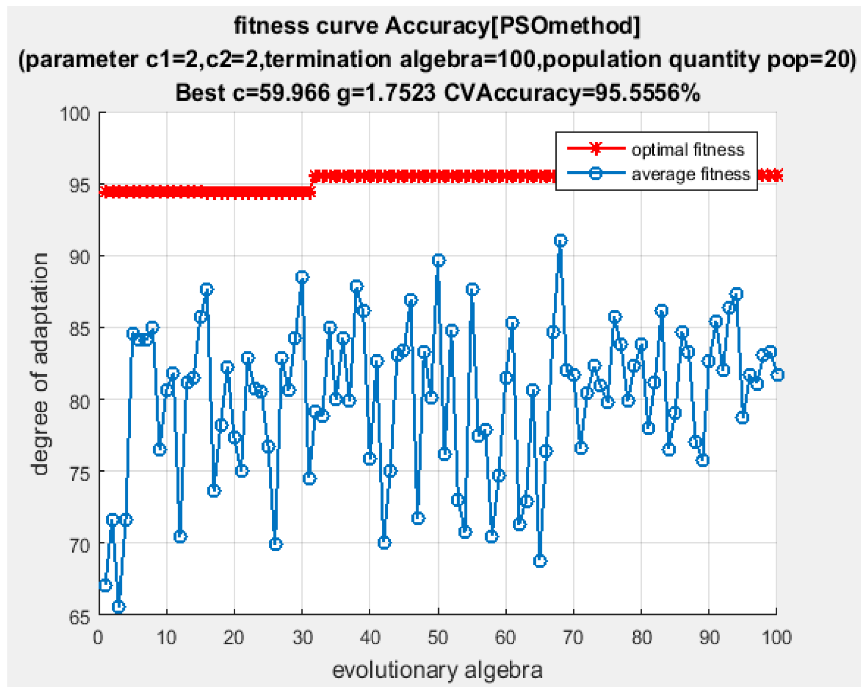
Learning factors $c_1$ and $c_2$ control the degree of interaction between the individual experience and the population experience, which reflects the information exchange between the groups. The appropriate choice of $c_1$ and $c_2$ can not only speed up the search but also avoid the whole population plunging into the local optimum. Learning factors generally take a fixed constant value [48], according to experience. In this paper, let $c_1=c_2=2$. 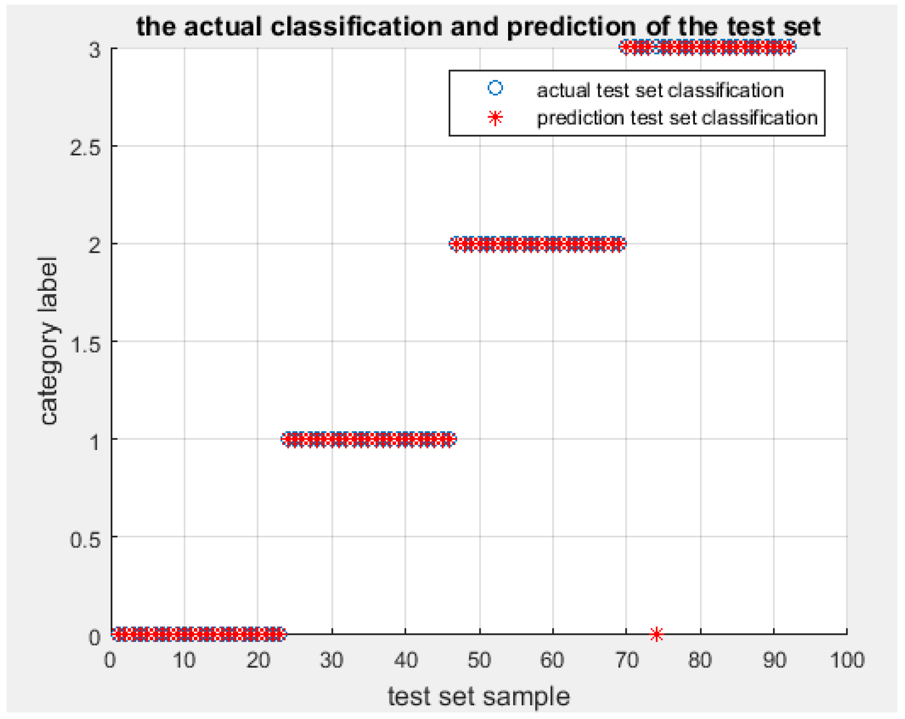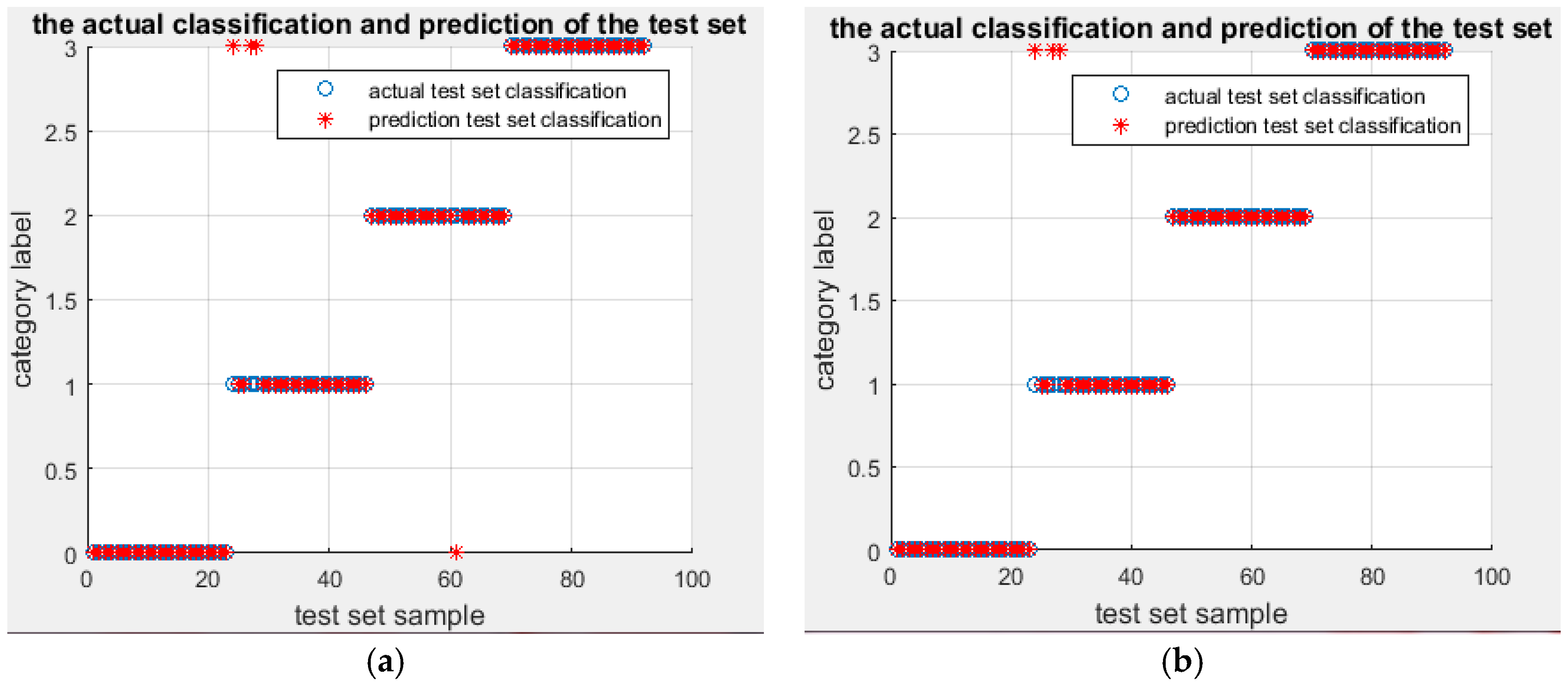The classification results of DFWT using IEMD-PSO-SVM are shown in Figure 3 and Figure 4.

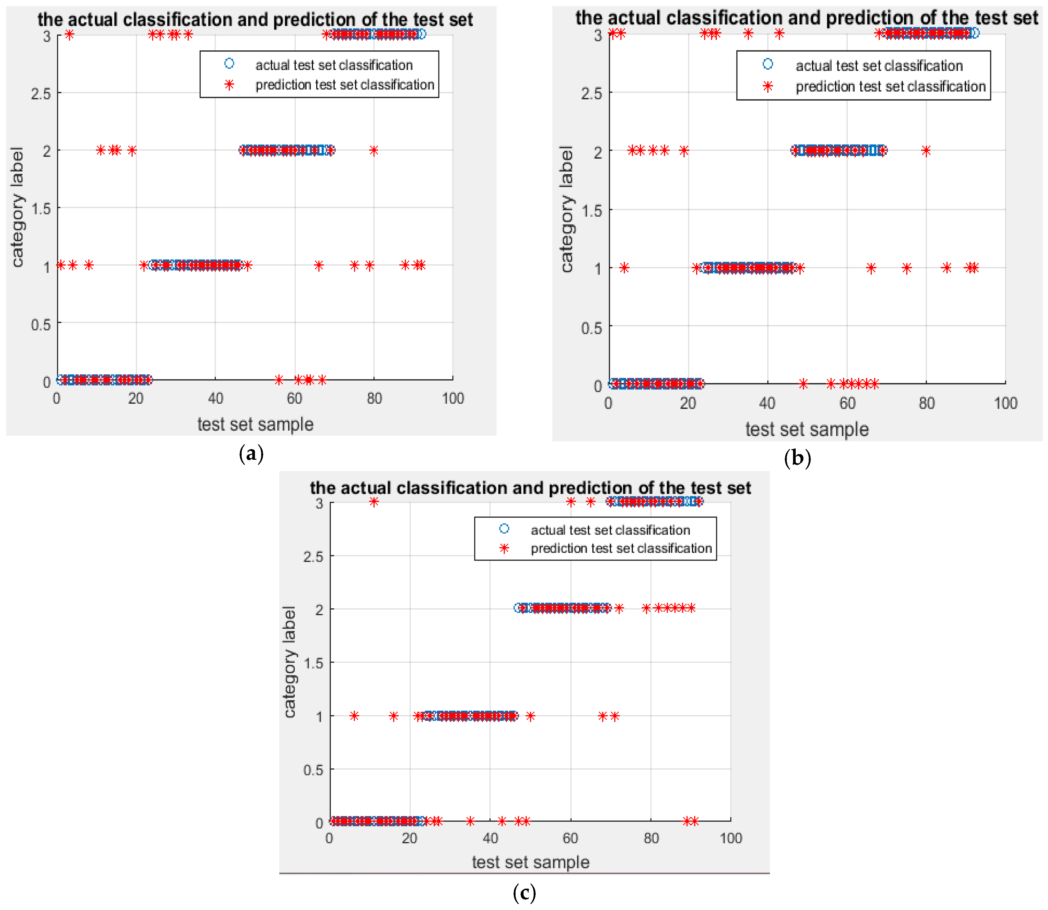
From Figure 3 and Figure 4, it can be seen that the testing accuracy of the SVM optimized by PSO is 95.5556%, and the optimal parameters are: $\mathrm{C}=59.966$ and $g=1.75228$. Only one sample is misclassified. The training accuracy at this time reaches 100% and the testing accuracy at this time also reaches 98.913%, with the correct rate of fault classification being very high. In order to illustrate the superiority of the proposed algorithm, the same energy entropy of the same vibration signals are classified by GridSearch-SVM (the parameters of SVM are optimized by GridSearch) and genetic algorithm (GA)-SVM (the parameters of SVM are optimized by Genetic Algorithm), and the recognition results are shown in Figure 5.

It can be seen that four samples are misclassified by the IEMD-GA-SVM model, while three samples are misclassified by IEMD-GridSearch-SVM. The testing accuracies are, respectively, 95.6522% and 96.7391%.

In a similar way, the energy entropy calculated after the same vibration signals being decomposed by EMD can be put into the PSO-SVM, GridSearch-SVM and GA-SVM, and the classification results are shown in Figure 6 and

Table 9. Comparison of IEMD-PSO-SVM with other commonly used classifiers.

Item	$\mathit{C}$	$\mathit{g}$	Elapsed Time (s)	Accuracy of Training Set	Accuracy of Testing Set	False Alarm Rate
EMD-GA-SVM	43.9431	2.1386	42.0268	98.8889% (178/180)	69.5652% (64/92)	9.7826% (9/92)
EMD-GridSearch-SVM	11.3137	0.5	14.8790	86.1111% (155/180)	68.4783% (63/92)	9.7826% (9/92)
EMD-PSO-SVM	68.7124	1.68153	39.2353	98.8889% (178/180)	71.7391% (66/92)	8.6956% (8/92)
IEMD-GA-SVM	29.8145	0.98656	46.3340	100% (180/180)	95.6522% (88/92)	1.0869% (1/92)
IEMD-GridSearch-SVM	16	2	15.3525	100% (180/180)	96.7391% (89/92)	0
IEMD-PSO-SVM	59.966	1.75228	25.6413	100% (180/180)	98.913% (91/92)	0

.

It can be seen that the promotion ability of EMD-GA-SVM, EMD-GridSearch-SVM and EMD-PSO-SVM was not high. Furthermore, the corresponding recognition accuracy decomposed by EMD was much lower than that by IEMD. The promotion ability of IEMD-GA-SVM and IEMD-GridSearch-SVM was less than that of IEMD-PSO-SVM. Thus, on the whole, the IEMD-PSO-SVM algorithm is better in diagnostic performance.

6. Conclusions

In this paper, aiming at the fact that misalignment fault samples are not enough to diagnosis, Solidworks and Adams are used to simulate the working conditions of DFWT to obtain the characteristic signals. After eliminating the end effects of EMD by using IEMD, the IEMD energy entropy of the vibration signals are extracted as the fault features. SVM, which is good at small sample learning, is used as the classifier to identify the misalignment. The parameters of SVM are optimized by the PSO algorithm. The results show that the fault diagnosis accuracy of misalignment of DFWT is higher. The effectiveness of the model is proved.