Energy, Exergy and Economic Evaluation Comparison of Small-Scale Single and Dual Pressure Organic Rankine Cycles Integrated with Low-Grade Heat Sources

Abstract

Low-grade heat sources such as solar thermal, geothermal, exhaust gases and industrial waste heat are suitable alternatives for power generation which can be exploited by means of small-scale Organic Rankine Cycle (ORC). This paper combines thermodynamic optimization and economic analysis to assess the performance of single and dual pressure ORC operating with different organic fluids and targeting small-scale applications. Maximum power output is lower than 45 KW while the temperature of the heat source varies in the range 100–200 °C. The studied working fluids, namely R1234yf, R1234ze(E) and R1234ze(Z), are selected based on environmental, safety and thermal performance criteria. Levelized Cost of Electricity (LCOE) and Specific Investment Cost (SIC) for two operation conditions are presented: maximum power output and maximum thermal efficiency. Results showed that R1234ze(Z) achieves the highest net power output (up to 44 kW) when net power output is optimized. Regenerative ORC achieves the highest performance when thermal efficiency is optimized (up to 18%). Simple ORC is the most cost-effective among the studied cycle configurations, requiring a selling price of energy of 0.3 USD/kWh to obtain a payback period of 8 years. According to SIC results, the working fluid R1234ze(Z) exhibits great potential for simple ORC when compared to conventional R245fa.

1. Introduction

In the last decades, the interest in improving energy efficiency of industrial processes has increased and new technologies have been proposed to reduce the consumption of fossil fuels [1,2]. To achieve this goal, new thermodynamic cycles have been proposed and some of them have been introduced in the market as competitive commercial alternatives to conventional heat-to-power cycles such as gas turbines and internal combustion engines. Some of these new thermodynamic cycles employ pure and zeotropic mixtures of organic fluids due to their low boiling temperatures, which results in an efficient utilization of the heat source [3,4,5]. In addition, new environmental friendly and low Global Warming Potential (GWP) fluids and nanofluids have been studied and tested to improve resources utilization [6,7]. The Organic Rankine Cycle (ORC) has emerged as an alternative technology to produce power from non-conventional energy sources, e.g., waste heat, solar radiation, geothermal heat and biomass. In fact, ORC is one the most widely used technologies for waste heat recovery in Europe, United States and Central America [8,9,10]. However, most of these commercial systems generate power above 200 kW [8,10,11]. Below this power output the profitability for power production from low grade heat sources via ORC needs further assessment [12,13]. For example a solar ORC system of 0.4–1.4 kW power output showed a payback period of 19 years. On the other hand an ORC system of 6–18 kW power output for heat recovery in the ceramic industry showed a payback period of 5 years [13,14].

In this context, several researchers have carried out studies to identify opportunities to improve ORC performance and increase its profitability at small scales. White and Sayma [12] investigated the effect of working fluid on the improvement of a small-scale ORC. They combined theoretical performance models, Computational Fluid Dynamics (CFD) and thermodynamic analysis for heat sources temperature in the range 87–127 °C. Their results showed that with an appropriate selection of the working fluid, ORC could generate between 2 kW and 30 kW without compromising its turbine performance. However, this study did not include an economic analysis to evaluate profitability and was also limited to a conventional ORC configuration. On the other hand, several analysis of the cycle components’ performance have been carried out. Li et al. [15] assessed conduction, convection and radiation heat losses of a small scale expander on the performance of an ORC. Other authors have designed, simulated and tested different types of expanders: scroll [16,17], screw [18,19,20] and radial [21,22,23,24].

Recently, some researchers have reconsidered the conventional configuration of ORC to increase its yield and profitability. The main concern of this reconfiguration is that the working fluid matches the temperature profile of the heat source [25]. Some modifications, such as the regenerative configuration, are able to increase power or thermal efficiency but reduce the heat recovered from the heat source. On the other hand, several researchers have argued that two pressure levels in the evaporation process would increase the overall performance of the system [26,27]. Therefore, it is necessary to develop new configurations which increase ORC performance and improve the exploitation of the thermal source.

Lecompte et al. [28] reviewed some alternative ORC configurations. Their study was focused on waste heat recovery ORC systems. Some of these configurations include: regenerative ORC, organic flash cycle, double organic flash cycle, trilateral cycle, ORC with zeotropic mixtures, transcritical ORC, ORC with multiple evaporation pressures, and cascade cycles. Compared to conventional ORC, configurations like ORC with multiple evaporation pressures and cascade cycles required additional equipment and instrumentation which increases direct and indirect costs. Other cycles like transcritical ORC could increase net power output but its thermal efficiency is low compared to conventional ORC, besides it requires additional equipment and control instruments to operate near critical conditions. From an operational point of view, the use of zeotropic mixtures implies a complex charging technique and the possible leaks in the cycle could significantly affect the balance of the system [29]. On the other hand, for small scale applications, Rahbar et al. [30] reported that conventional and regenerative ORC are the most studied configurations, and most of the previous research in this field have been focused on the application (solar, geothermal, etc.) coupled with the conventional configuration.

Many of the new configurations have been studied from the thermodynamic point of view, without taking into account its cost-effectiveness and power generation at small scale. In addition, some of the improvements mentioned above may not be competitive or profitable in relation to the conventional energy generation cycles or the conventional ORC, specially at small scale. For this reason, this paper proposes a comprehensive thermodynamic and economic study of a small scale dual pressure ORC configuration operating with low temperature waste heat recovery and generating a net power of less than 45 kW. The dual pressure ORC configuration was proposed by Lecompte et al. [28] and has been recently studied by Manente et al. [25]. The aim of this paper is to determine the optimum operation conditions of this configuration and compare it with two traditional ORC cycles: simple ORC and regenerative ORC, by analyzing the effect of the configuration, and working fluid on net power production, thermal efficiency, Specific Investment Cost (SIC) and Levelized Cost of Electricity (LCOE). A sensitivity analysis of the selling price of energy on the Net Present Value (NPV) is also presented.

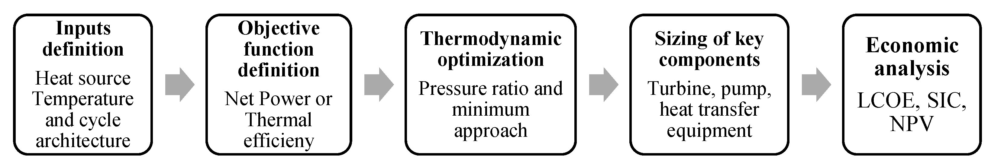
2. Materials and Methods

2.1. Working Fluid Selection

In this paper we consider the list of potential fluids in the working fluid database of REFPROP 9.1 [31]. Working fluids must satisfy Kyoto and Montreal Protocols, therefore the use of Chlorofluorocarbons (CFCs) and Hydro-chlorofluorocarbons (HCFCs) is forbidden due to their Ozone Depletion Potential (ODP). Additionally, ODP and GWP are typically employed as a restriction for working fluid selection. Working fluids with ODP above zero and GWP over 100 years above 150 are forbidden by European Union guidelines [32]. In this study, only pure substances are considered. In terms of safety, only fluids with low toxicity, low and low-mid flammability are considered. Thus, working fluids with a safety classification of A1, A2L according to the ASHRAE 34-2001 Standard are selected. Heat source temperature ranges from 100 °C to 200 °C, therefore only organic fluids with critical temperatures above 90 °C are considered. Previous studies [33,34] suggested that pressures might be between 0.1 and 2.5 MPa to make the ORC operation safe and profitable. When working pressures are outside of this range, additional control and safety equipment are required in heat exchangers, which increases capital cost and diminishes profitability. Based on the aforementioned criteria the working fluids R1234yf (2,3,3,3-Tetrafluoropropene), R1234ze(E) (trans-1,3,3,3-Tetrafluoropropene) and R1234ze(Z) (cis-1,3,3,3-tetrafluoroprop-1-ene) were selected.

2.2. Simulation Details

The present study focuses on the use of waste heat from industrial processes, which may be present in the form of exhaust gases from internal combustion engines (66–120 °C), annealing furnaces (66–230 °C), drying, curing and curing ovens (93–230 °C) and hot processed liquids and solids (32–232 °C) [34]. To ensure proper control of the integration between the heat source and the ORC, an intermediate thermal oil circuit is considered and Therminol 55 is used as the heat transfer fluid (HTF). The temperature of the source can be variable, however, stable conditions are guaranteed at the evaporator inlet with the use of HTF.

An optimization process was performed for the three proposed cycle configurations: simple ORC (Figure 1a), regenerative ORC (Figure 1b), and dual pressure ORC (Figure 1c). A simulation program was developed in MATLAB and the thermodynamic properties were calculated using REFPROP 9.1 [31].

Mass and energy balances were developed for each configuration and two independent optimization functions were defined: net power output and first law efficiency. These objective functions are given by Equations (1) and (2).

$${\dot{W}}_{net}=\sum {\dot{W}}_{turb,i}-\sum {\dot{W}}_{pump,i}$$

(1)

$${\eta }_{th}={\dot{W}}_{net}/{\dot{Q}}_{in}$$

(2)

where ${\dot{W}}_{turb,i}$, ${\dot{W}}_{pump,i}$, ${\dot{W}}_{net}$, ${\dot{Q}}_{in}$ and ${\eta }_{th}$ are the turbine power, pump power, net power, heat input and thermal efficiency, respectively.

The parameters and constraints considered in this study are presented in

Table 1. Parameters considered for the optimization process.

Parameter	Units	Value
Heat source temperature	°C	100–200
Pinch Point Temperature Difference	°C	10
Turbine isoentropic efficiency	°C	85
Pump isoentropic efficiency	°C	85
Condensation temperature	°C	40
Heat source fluid or Heat transfer fluid (HTF)	-	Therminol 55
Heat source mass flow rate	kg/s	1.0

. Two different conditions are considered for the turbine inlet temperature: superheated vapor and saturated vapor (See Figure 2). Therminol 55 is considered as the heat source, and liquid water is considered as the cooling fluid in the condenser. The thermodynamic optimization procedure is shown in Figure 3.

In this paper the exergy efficiency and the exergy destruction are calculated for each combination of cycle and working fluid. The exergy efficiency is given by:

$${\eta }_{\mathrm{exergy}}={\dot{W}}_{\mathrm{net}}/E_{in}$$

(3)

In the previous equation $E_{in}$ is the change in exergy of the heat source which is equivalent to the exergy input. The exergy input represents the maximum amount of useful work that can be done by the cycle. The exergy balance for a control volume is given by [35]:

$${\displaystyle \frac{d{E}_{cv}}{dt}}=\sum _j{\dot{E}}_{qj}-{\dot{W}}_{cv}+\sum _i{\dot{m}}_i{e}_{fi}-\sum _e{\dot{m}}_e{e}_{fe}-{\dot{E}}_d$$

(4)

with:

$${\dot{E}}_{qj}=\left(1-T_o/T_j\right){\dot{Q}}_j$$

$$e_f=h-h_o-T_o\left(s-s_o\right)+V^2/2+gz$$

where ${\dot{E}}_{qj}$ is the exergy input due to heat transfer, ${\dot{W}}_{cv}$ is the work done by the system, $e_f$ is the specific exergy of the fluid and ${\dot{E}}_d$ is the exergy destruction.

2.3. Sizing of Components

2.3.1. Turbine and Pump

The size of the turbine is defined in terms of the power generated (${\dot{W}}_{turb}$), which is determined by means of Equation (5) in terms of the mass flow rate of the turbine ${\dot{m}}_{turb}$ and the enthalpies at the turbine inlet $h_{in}$ an outlet $h_{out}$.

$${\dot{W}}_{turb}={\dot{m}}_{turb}\left(h_{in}-h_{out}\right)$$

(5)

In the case of the pump, the size is defined in terms of the power consumed, which is determined by means of Equation (6).

$${\dot{W}}_{pump}={\dot{m}}_{pump}\left(h_{out}-h_{in}\right)$$

(6)

where ${\dot{W}}_{pump}$ is the pump power, ${\dot{m}}_{turb}$ is the mass flow rate across the pump, $h_{in}$ and $h_{out}$ are the enthalpies at the pump inlet and outlet, respectivelty.

2.3.2. Heat Transfer Equipment

To determine the size of the heat transfer equipment, the overall heat transfer area is calculated for each heat exchanger: boiler, condenser and internal heat exchanger. To calculate the overall heat transfer area, the boiler is divided into three zones: preheating, evaporation and superheating. The thermal oil in the boiler is considered as a single phase fluid. On the other hand, the working fluid in the preheating and superheating zones is treated as a single phase fluid, and as a two phase fluid in the evaporation zone. The condenser is divided into two zones: the cooling zone where the working fluid exists in a single phase, and the condensing zone where the working fluid is treated as a two phase fluid. The cooling water in the condenser, is considered as a single phase fluid. Finally, in the internal heat exchanger the working fluid is considered as a single phase fluid.

The overall heat transfer area (A) of each heat exchanger is the sum of heat transfer areas of all its zones, which is computed via the Number of Transfer Units ($\epsilon$-NTU) and Log-Mean Temperature Difference (LMTD) method according to Equation (7) [36].

$$A=\frac{Q}{U·\mathrm{\Delta }{T}_{ml}}$$

(7)

where $\mathrm{\Delta }{T}_{ml}$ is the logarithmic mean temperature difference between the hot side and the cool side and U is overall heat exchanger coefficient, which is calculated by following the thermal resistance approach in Equation (8) [36,37].

$$\frac{1}{U}=\frac{1}{h_{cs}}+R_w+\frac{1}{h_{hs}}$$

(8)

where $R_w$ is the resistance of the material of the wall, $h_{cs}$ is the heat exchanger coefficient of the cold side, and $h_{hs}$ is the heat exchanger coefficient of the hot side.

For the single phase zone of the boiler, the condenser and the internal heat exchanger, the heat transfer coefficient ($h_{sp}$) is calculated by Equation (9) [38].

$${\mathrm{Nu}}_{sp}=\frac{h_{sp}{D}_h}{k}=0.78·{\mathrm{Re}}^{0.5}{\mathrm{Pr}}^{1/3},10<\mathrm{Re}<20,000$$

(9)

where $D_h$ is the hydraulic diameter, k is thermal conductivity of the fluid, $\mathrm{Re}$ is the the Reynolds number and $\mathrm{Pr}$ is the Prandtl number.

In the two phase zone of the boiler, two phase heat transfer coefficient ($h_{tp}$) is calculated by means of Equation (10) [39].

$${\mathrm{Nu}}_{tp}=\frac{h_{tp}{D}_h}{k_l}=0.00187·{\left(\frac{q·d_o}{k_l}\right)}^{0.56}{\left(\frac{h_{fg}{d}_o}{{\alpha }_l^2}\right)}^{0.31}{\mathrm{Pr}}^{0.33}$$

(10)

where $k_l$ is thermal conductivity of the liquid phase, q is heat flux, $d_0$ is bubble departure diameter, $h_{fg}$ is specific latent heat of vaporization and ${\alpha }_l$ is thermal diffusivity of the liquid phase.

In the two phase zone of the condenser, the heat transfer coefficient ($h_{tp}$) is calculated by Equation (11) [40], where ${\mathrm{Re}}_{eq}$ is Reynolds number for equivalent mass flow ($G_{eq}$). ${\mathrm{Re}}_{eq}$ and $G_{eq}$ are calculated by means of Equations (12) and (13), respectively.

$${\mathrm{Nu}}_{tp}=\frac{h_{tp}{D}_h}{k_l}=4.118·{\mathrm{Re}}_{eq}^{0.4}·{\mathrm{Pr}}_l^{0.33}$$

(11)

$${\mathrm{Re}}_{eq}=\frac{G_{eq}·D_h}{{\mu }_l}$$

(12)

$$G_{eq}=G\left[1-x_m+x_m{\left(\frac{{\rho }_l}{{\rho }_v}\right)}^{1/2}\right]$$

(13)

where ${\mu }_l$ is dynamic viscosity of the liquid phase, $x_m$ is vapor quality, ${\rho }_l$ and ${\rho }_v$ are vapor and liquid phase densities, respectively, and ${\mathrm{Pr}}_l$ is the Prandtl number of the liquid phase.

2.4. Cost Structure and Estimation

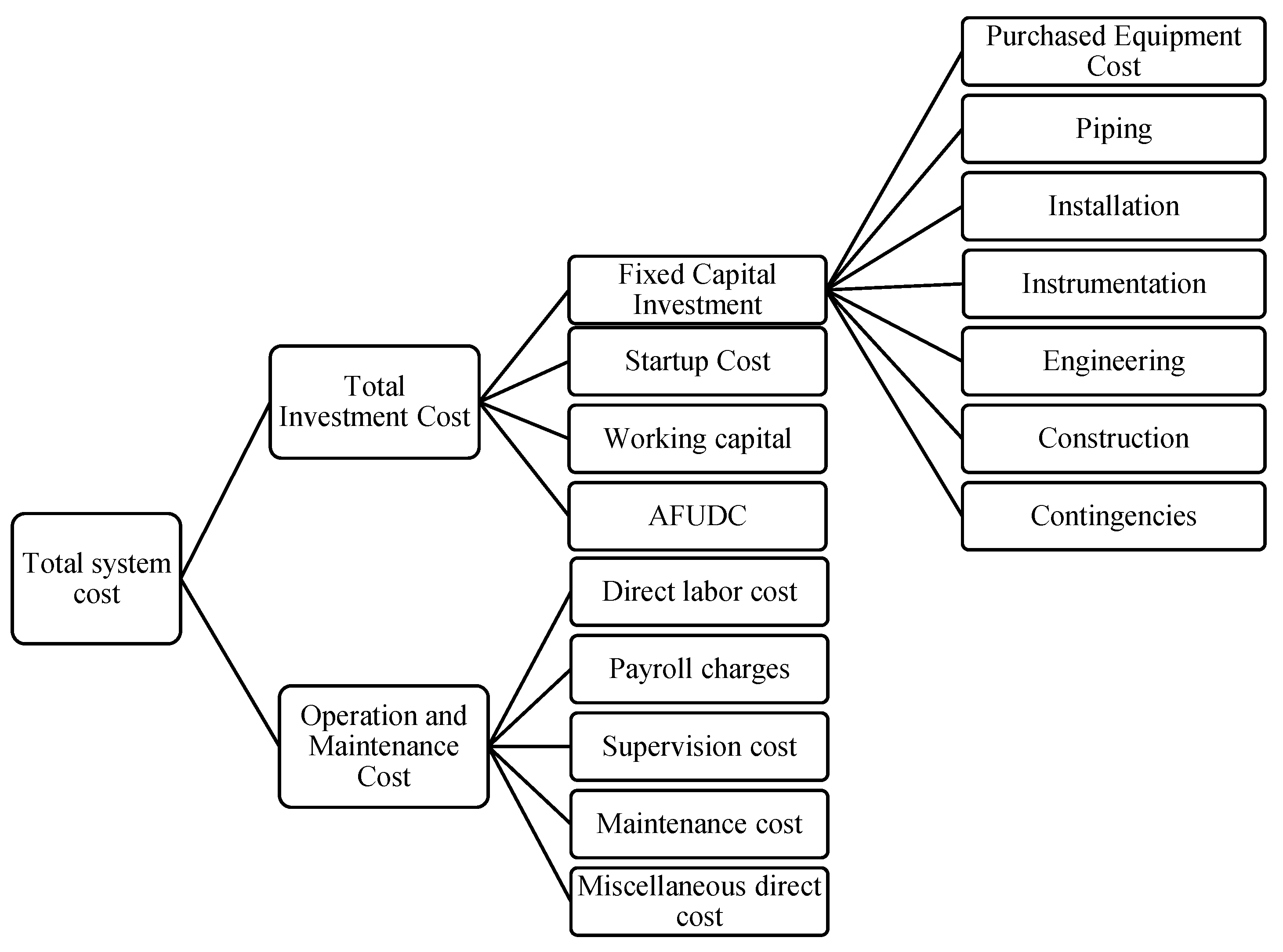
2.4.1. Total Investment Cost

The aim of this section is to evaluate the results of the thermodynamic optimization from an economic point of view. Thus, the total investment and the cost of energy production is determined from the cost of the main components of the cycle: heat exchangers, turbine and pump. On the other hand, the cost of the startup, working capital, other fixed capital investment components, and operation and maintenance costs are determined following the assumptions and suggestions proposed by Bejan and Tsatsaronis [41]. The cost structure for the economic analysis is presented in Figure 4. The description of the cost structure is presented below.

For Purchased Equipment Cost (PEC), a market and literature search was performed and a cost function was built. The structure of the cost function follows the methodology proposed by Bejan and Tsatsaronis [41]. In this methodology, the cost of each component is calculated from a specific parameter as it is shown in Equation (14).

$$C=C_{ref}{\left(\frac{B}{B_{ref}}\right)}^n$$

(14)

where B is the specific parameter (area or power), $C_{ref}$ is the reference cost of $B_{ref}$, y n is and exponent for the cost scaling. Values for B, $B_{ref}$, $C_{ref}$ and n are presented in

Table 2. Values for B, $B_{ref}$, $C_{ref}$ and n for the cost function of the ORC components.

Component	Parameter	Units	${\mathit{B}}_{\mathit{r}\mathit{e}\mathit{f}}$	${\mathit{C}}_{\mathit{r}\mathit{e}\mathit{f}}$ (USD)	n	Reference
Turbine	Power	kW	0.1	500	0.73	[42]
Heat exchangers	Area	m${}^2$	0.12	304	0.69	[43]
Pump	Power	kW	0.3	1000	0.45	[34]

. The heat transfer areas are calculated by following the heat transfer equations for brazed plate heat exchangers presented in the previous section. The remain components of the fixed capital investment and the total investment are determined as a percentage of the total investment cost. A description of these costs and their values is presented in

Table 3. Remaining investment costs.

Parameter	Percentage	Base for Percentage Calculation	Reference
Piping	9%	Purchased Equipment Cost	[44]
Installation of equipment	20%	Purchased Equipment Cost	[41]
Instrumentation and controls	5%	Purchased Equipment Cost	[44]
Electrical equipment	4%	Purchased Equipment Cost	[44]
Civil and structural work	5%	Purchased Equipment Cost	[44]
Engineering and supervision	30%	Purchased Equipment Cost	[41]
Construction	10%	Direct costs	[41]
Contingencies	15%	Fixed Capital Investment	[41]
Startup cost	1%	Fixed Capital Investment	[44]
Working capital	3%	Purchased Equipment Cost	[44]
AFUDC	15%	Fixed Capital Investment	[41]

.

2.4.2. Operation and Maintenance Costs

Operation and maintenance costs comprise the following expenses [45]: direct labor, supervision, payroll charges, maintenance, miscellaneous direct costs. The detail of the calculation of these costs is presented in

Table 4. Remaining operation and maintenance costs. Values taken from [45].

Parameter	Percentage	Base
Payroll charges	35%	Direct labor and supervision costs
Supervision costs	15%	Direct labor cost
Maintenance costs	6%	Fixed Capital Investment
Operating supplies	5–7%	Direct labor cost
Laundry	10–15%	Direct labor cost
Laboratory	10–15%	Direct labor cost

except for direct labor costs, which are calculated by using Equation (15). In this equation $C_h$ is the cost of the time, $H_A$ is the annual working time, and $N_L$ is the number of workers. $C_h$ is set as 3 USD/h, a value of 2080 h/worker is set for $H_A$, and $N_L$ is determined for each configuration using the Ulrich method [45]: 0.6 for the first configuration (Figure 1a), 0.65 for the second configuration (Figure 1b), and 0.65 for the third configuration (Figure 1c).

$$\mathrm{Direct}\mathrm{labor}\mathrm{costs}=C_h·N_L·H_A$$

(15)

2.4.3. Levelized Cost of Electricity and Net Present Value

LCOE and SIC are determined to compare the performance of selected working fluids and configurations from an economic point of view. LCOE represents the minimum cost of the kWh to cover the necessary costs for generating electricity: initial investment, operation and maintenance, fuel costs, insurance, etc. [41]. LCOE is calculated as it is shown in Equation (16) and SIC is determined from Equation (17).

$$LCOE=\frac{{\displaystyle \sum _{n=0}^N}\frac{C_n+O\&M_n+F{E}_n}{{(1+r)}^n}}{{\displaystyle \sum _{n=0}^N}\frac{E_n}{{(1+r)}^n}}$$

(16)

$$SIC=\frac{TEC+O\&M}{{\dot{W}}_{net}}$$

(17)

where $C_n$ are the investment expenditures of the year of operation (n), $O\&M$ are the operation and maintenance expenditures, $F{E}_n$ are the fuel expenditures, $E_n$ is the cash income from electricity generation, r is the effective discount rate and N is the lifetime period.

Another parameter employed to assess economic profitability is Net Present Value (NPV), which is defined as the present value of a number of future cash flows from an investment [41]. NPV is calculated as:

$$NPV=\sum _{n=1}^N{Y}_n{\left(1+r\right)}^n-I_0$$

(18)

where $Y_n$ is the cash flow of every year of operation (n), $I_0$ is the initial investment, and r is the effective discount rate. The economic assumptions for the economic evaluation are [34]:

• The lifetime period is 20 years
• The capacity factor is set to 85%
• Average general inflation rate is 5%
• Average income taxes interest rate is 33%
• Cost of capital or interest rate, 5%
• Straight line depreciation is assumed over the lifetime of the ORC

3. Results and Discussion

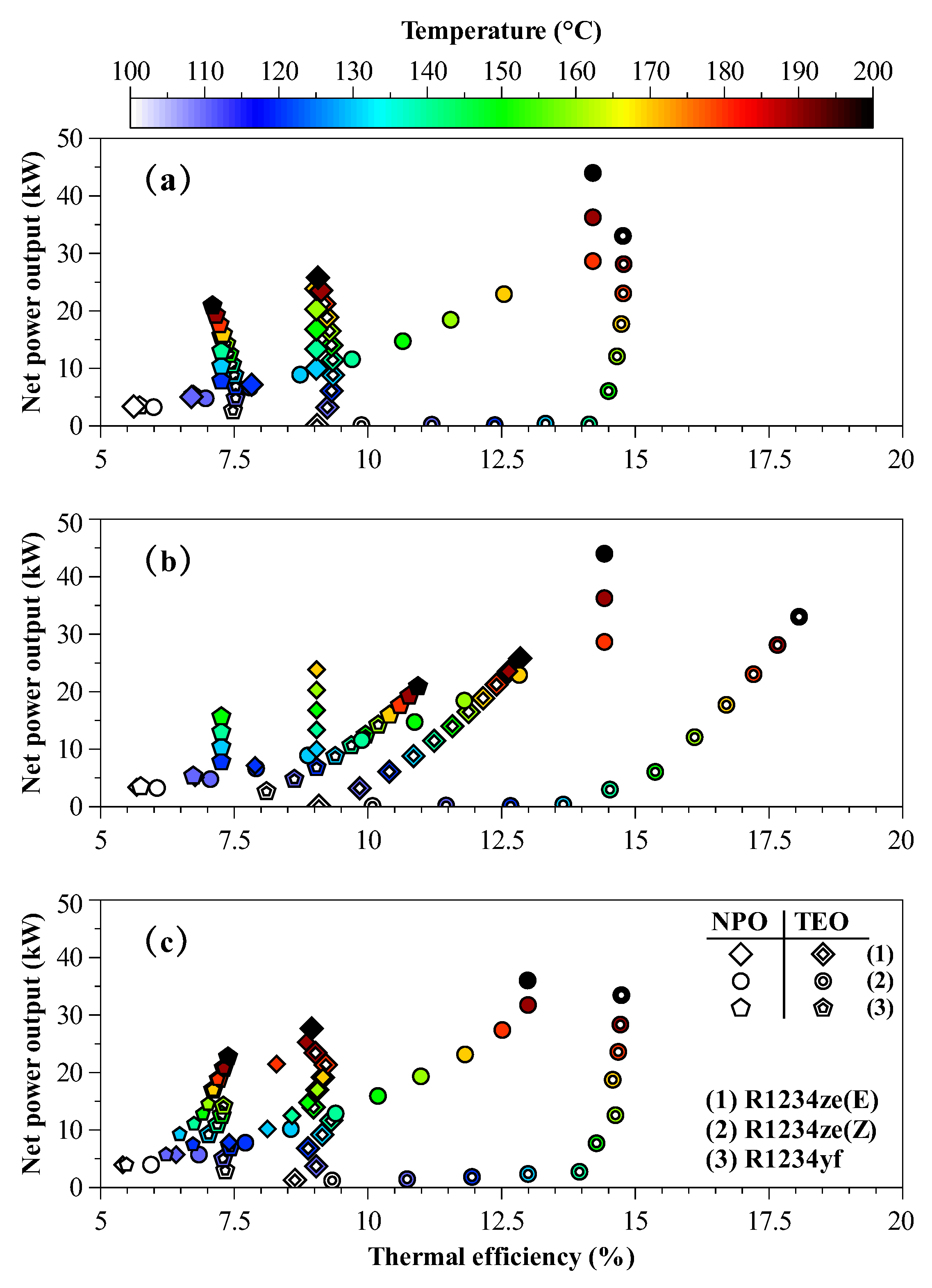
3.1. Power and Thermal Efficiency Optimization

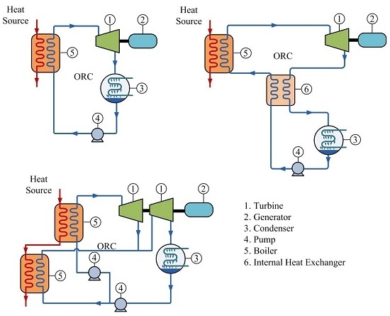
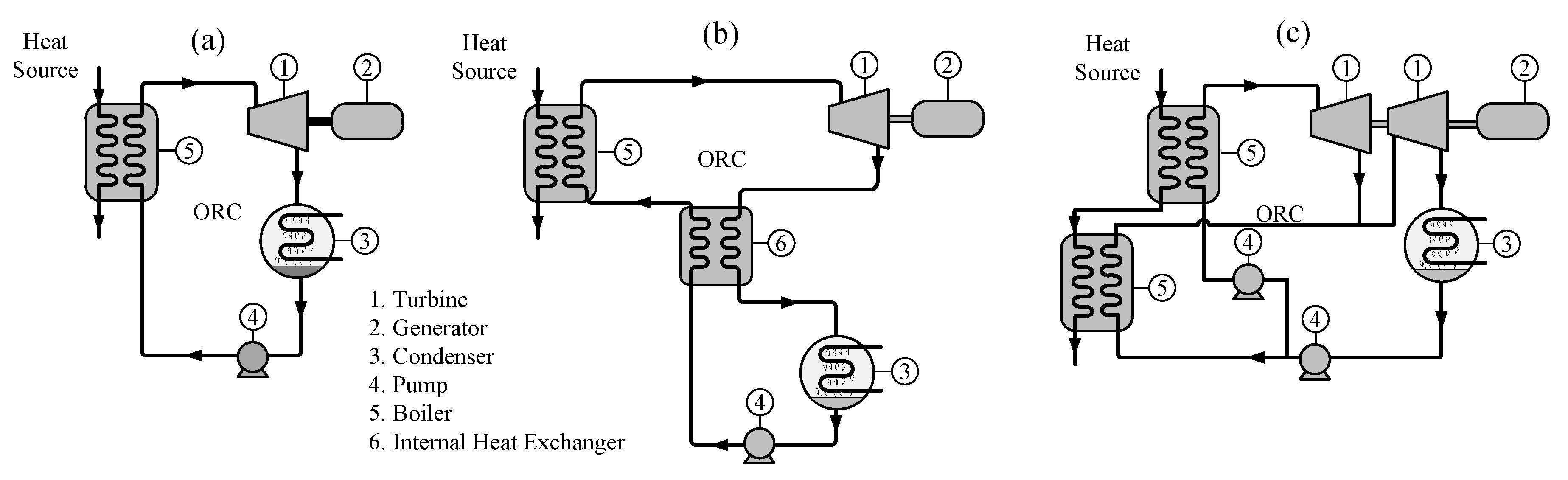
3.1.1. Simple ORC

In the case of simple ORC (Figure 5a), fluids develop almost the same net power output and thermal efficiency when heat source temperature is below 130 °C and net power is optimized. However, thermal efficiency is higher for R1234ze(Z) and R1234ze(E) when thermal efficiency is optimized. Nevertheless, increasing thermal efficiency adversely affects the net power for R1234ze(Z) with a reduction from 3.3 to 0.1 kW at 100 °C, and from 6.6 to 0.2 kW at 130 °C. The optimization of thermal efficiency leads to a superheated condition in the turbine inlet, this increment in turbine inlet temperature reduces the mass flow rate in the evaporator at the same pinch point conditions [46]. When the heat source temperature is below 130 °C, R1234ze(Z) requires low evaporation pressures, which leads to rather limited enthalpy drops in the turbine which results in a low power output.

When net power output is optimized above 130 °C, R1234yf reaches its maximum pressure as reported in literature (25 bar) [33,34], which slightly increases the net power of the cycle from 10.4 to 20.9 kW, but at a constant low thermal efficiency of 7.1–7.3%. Those values are quite similar to those obtained when the thermal efficiency is optimized. This is due to the pressure limit and the low critical temperature of R1234yf, which implies that the optimum net power and efficiency occurs simultaneously. This situation is also present in R1234ze(E) and R1234ze(Z), but their higher critical temperatures allow to develop higher net power and higher thermal efficiency. Moreover, since R1234ze(Z) has the highest critical temperature, this fluid develops the highest net power and thermal efficiency among the studied fluids. It is important to point out that R1234ze(Z) develops the highest net power because its thermodynamic condition at the turbine inlet is saturated vapor at higher temperatures.

3.1.2. Regenerative ORC

For the regenerative ORC (Figure 5b) results are similar to those obtained for the simple ORC when net power is optimized at heat source temperatures up to 160 °C for R1234yf, and up to 180 °C for R1234ze(E). This is because there is no heat recovery in the internal heat exchanger. Above this temperatures, the turbine outlet temperature increases and the internal heat exchanger is active, which reduces heat consumption in the evaporator and increases thermal efficiency. In addition, when thermal efficiency is optimized, the working fluids achieve the highest thermal efficiency at the superheated vapor condition at the turbine outlet. This condition leads to higher turbine outlet temperatures which activate the internal heat exchanger and the thermal efficiency is therefore increased. This explains why the net power optimization results have opposite trends to those obtained by the thermal efficiency optimization. However, is important to mention that even though the internal heat exchanger increases efficiency, it does not increase net power as can be seen from Figure 5.

3.1.3. Dual Pressure ORC

According to Figure 5c, the dual pressure ORC has the highest optimum net power output, up to 5.3 kW, when the heat source temperature is below 130 °C. Above 130 °C, as suggested in literature [33,34], the net power output of the dual pressure ORC is limited by the maximum operation pressure, 25 bar. When the maximum evaporation pressure is reached, the turbine inlet temperature has to be increased to obtain a higher power output. However, as the intermediate pressure is also increased, the power consumption in the pumps increases as well, and the dual pressure ORC generates less net power output than the other two cycles (simple and regenerative ORC). Simple and regenerative ORC develop the same power output but with different thermal efficiencies. Based on the results, the dual pressure ORC is an attractive cycle at heat source temperatures lower than 130 °C, since the regenerative and simple ORC achieve the highest net power output above 130 °C, up to 44.0 kW.

Results are compared with those obtained by Manente et al. [25] at 100 and 150 °C (

Table 5. Thermal efficiency comparison of the net power and thermal efficiency optimization results with the performance of the simple and the dual pressure ORC presente by Manente et al. [25]. NPO = Net power optimization. TEO = Thermal efficiency optimization. UN = Unconstrained scenario. CON = Constrained scenario.

	Thermal Efficiency Simple ORC (%)				Thermal Efficiency Dual Pressure ORC (%)
Heat source temperature (°C)	NPO	TEO	UN	CON	NPO	TEO	UN	CON
R1234yf
100	5.7	7.5	5.4	6.0	5.5	7.3	5.5	6.6
R1234ze(E)
100	5.6	9.0	5.5	6.0	5.4	8.6	5.6	6.8
150	9.0	9.3	9.8	10.5	8.9	9.0	9.9	10.4
R1234ze(Z)
100	6.0	9.9	5.8	5.9	5.9	9.3	5.8	7.1
150	10.6	14.5	10.3	10.3	10.2	14.3	10.5	10.9

). The results show that the net power optimization efficiencies are very close to the unconstrained scenario proposed by Manente et al. [25]. In this scenario the dual pressure ORC develops a lower thermal efficiency than simple ORC. Furthermore, R1234ze(Z) is the working fluid with the highest thermal efficiency and this trend is confirmed by Manente et al. [25] in both constrained and unconstrained scenarios.

Table 6. Optimum cycle configuration for different working fluids based on the individual optimization of net power and thermal efficiency. DP = Dual pressure ORC, S = Simple ORC, R = Regenerative ORC.

	R1234yf			R1234ze(Z)			R1234ze(E)
Heat Source Temperature (°C)	Net Power (kW)	Thermal Efficiency (%)	Cycle	Net Power (kW)	Thermal Efficiency (%)	Cycle	Net Power (kW)	Thermal Efficiency (%)	Cycle
Net Power Optimized
100	4.0	5.5	DP	4.0	5.9	DP	4.0	5.4	DP
110	5.7	6.2	DP	5.7	6.8	DP	5.7	6.4	DP
120	7.8	7.3	R	7.8	7.7	DP	7.8	7.4	DP
130	10.4	7.3	R	10.2	8.6	DP	10.2	8.1	DP
140	13.0	7.3	R	12.9	9.4	DP	13.4	9.0	R
150	15.7	7.3	R	15.9	10.2	DP	16.8	9.0	R
160	14.5	7.0	DP	19.3	11.0	DP	20.3	9.0	R
170	17.0	7.1	DP	23.1	11.8	DP	23.8	9.0	R
180	18.8	7.2	DP	28.7	14.4	R	21.6	7.6	R
190	20.8	7.3	DP	36.3	14.4	R	25.3	8.8	DP
200	22.7	7.4	DP	44.0	14.4	R	27.7	8.9	DP
Thermal Efficiency Optimized
100	2.6	8.1	R	0.1	10.1	R	0.1	9.1	R
110	4.8	8.6	R	0.2	11.5	R	3.2	9.8	R
120	6.8	9.0	R	0.1	12.7	R	6.1	10.4	R
130	8.8	9.4	R	0.4	13.7	R	8.8	10.9	R
140	10.6	9.7	R	3.0	14.5	R	11.5	11.2	R
150	12.5	10.0	R	6.1	15.4	R	14.0	11.6	R
160	14.2	10.2	R	12.1	16.1	R	16.5	11.9	R
170	15.9	10.4	R	17.7	16.7	R	18.9	12.2	R
180	17.6	10.6	R	23.0	17.2	R	21.2	12.4	R
190	19.3	10.8	R	28.1	17.7	R	23.5	12.6	R
200	20.9	10.9	R	33.0	18.1	R	25.8	12.8	R

shows results for individual optimization of net power and thermal efficiency and the optimum configuration for each heat source temperature studied. By optimizing net power output, R1234z(E) and R134ze(Z) are the working fluids that maximize power and thermal efficiency. At 200 °C, R1234ze(Z) reaches up to 44.0 kW of net power output while R1234ze(E) develops up to 27.7 kW, and R1234yf develops just 22.7 kW. However, when thermal efficiency is maximized, the maximum power obtained for R1234ze(Z) reduces to 33.0 kW. A similar trend is also observed for R1234ze(E) and R1234yf. Thus, the optimization of thermal efficiency implies a sacrifice of net power output.

On the other hand, when power is optimized thermal efficiencies are lower than the optimized efficiencies (Table 6), which means that the optimization of the net power also involves a sacrifice of thermal efficiency for the studied cycles.

This trend is also confirmed by Manente et al. [25] (Table 5). The change from unconstrained to a constrained scenario in the dual pressure ORC, for R1234ze(Z), causes a reduction of net power output from 961 to 892 kW at 100 °C and from 3778 to 3707 kW at 150 °C. In the case of R1234ze(E), net power was reduced from 966 kW to 862 kW at 100 °C, and from 4382 to 3513 kW at 150 °C.

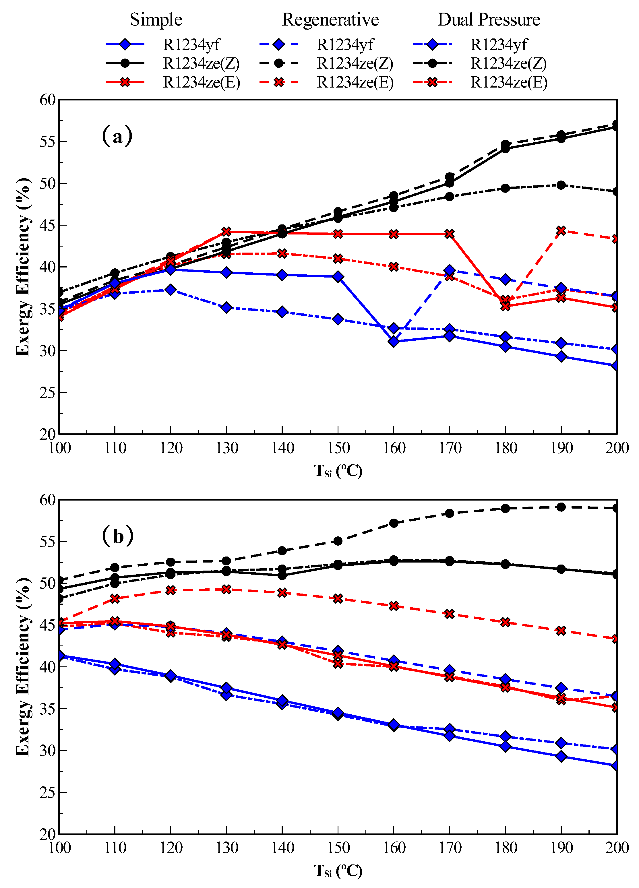
3.2. Exergy Efficiency and Exergy Destruction

Figure 6a show the exergy efficiency for the three ORC configurations and working fluids when net power output is optimized. There are no major differences in exergy efficiency below 120 °C. This is caused by the combination of two factors: first, fluids reach optimum net power output with saturated vapor condition at the turbine inlet, and second, the evaporation pressures is very close to each other. Above 120 °C R1234yf reaches the maximum pressure and its exergy efficiency starts decreasing because its relatively low critical temperature. The same holds for R1234ze(E) above 140 °C. This observable does not take place in the case of R1234ze(Z) because its higher critical temperature allows reaching higher exergy efficiencies as the heat source temperature increases.

Regarding ORC configurations, the use of regenerator significantly increases exergy efficiency. The improvement is noticeable in R1234ze(E) and R1234yf due to their critical temperature and pressure limitations. According to Figure 6b the effect is much more remarkable when the thermal efficiency is optimized because the superheated vapor condition at the turbine inlet increases the turbine outlet temperature and activates the recovery heat exchanger, which reduces the heat input and the generation of entropy in the evaporator.

Finally, R1234ze(Z) is the working fluid with the highest exergy efficiency. Its superior performance becomes more evident when thermal efficiency is optimized, rather than when the power is optimized. Below 120 °C, R1234ze(Z) has a higher exergy efficiency when is used as working fluid in the dual pressure ORC. Above 130 °C, regenerative ORC is the configuration that increases its exergy efficiency.

The inclusion of the internal heat exchanger reduces the heat transfer in the evaporator therefore, the entropy generation and the irreversibilities are reduced as well. However, according to Manente et al. [25], the goal is to recover the highest amount of energy following the most efficient way. As previously mentioned, the regenerative configuration is able to increase performance but reduces the heat recovered from the heat source. Another issue of this high efficiency combination is that the net power output is sacrificed, specially at lower temperatures, where the cycle generates low power. This issue leads to higher LCOE as is evident from the economic analysis.

3.3. Levelized Cost of Electricity - LCOE

As presented above, net power and thermal efficiency optimization show opposite trends. To examine the profitability of each approach, LCOE and SIC are determined. LCOE values for net power optimization and thermal efficiency optimization are presented in

Table 7. LCOE for each cycle configuration in USD/kWh obtained from the individual optimization of net power output and thermal efficiency. DP = Dual pressure ORC, S = Simple ORC, R = Regenerative ORC.

	R1234yf			R1234ze(E)			R1234ze(Z)
Heat Source Temperature (°C)	S	R	DP	S	R	DP	S	R	DP
Net Power Optimized
100	0.80	1.11	0.92	0.78	1.11	0.84	0.80	1.09	0.90
110	0.62	0.64	0.74	0.60	0.81	0.67	0.62	0.80	0.72
120	0.51	0.52	0.64	0.49	0.64	0.56	0.51	0.62	0.60
130	0.46	0.47	0.58	0.42	0.52	0.49	0.42	0.51	0.52
140	0.43	0.44	0.53	0.36	0.43	0.43	0.38	0.43	0.47
150	0.49	0.50	0.49	0.32	0.37	0.39	0.35	0.39	0.43
160	0.50	0.54	0.46	0.29	0.33	0.35	0.34	0.36	0.40
170	0.39	0.38	0.44	0.26	0.29	0.32	0.44	0.46	0.38
180	0.37	0.36	0.42	0.24	0.26	0.30	0.43	0.43	0.36
190	0.36	0.34	0.40	0.22	0.24	0.28	0.30	0.30	0.35
200	0.35	0.32	0.38	0.22	0.23	0.27	0.29	0.28	0.33
Thermal Efficiency Optimized
100	0.96	1.45	1.02	9.78	63.74	1.64	8.80	47.16	1.61
110	0.68	0.88	0.76	6.52	35.54	1.41	0.81	1.21	0.84
120	0.57	0.68	0.64	9.38	66.72	1.17	0.56	0.71	0.61
130	0.51	0.57	0.57	3.72	15.75	0.99	0.47	0.55	0.53
140	0.46	0.50	0.53	5.14	1.36	0.90	0.42	0.47	0.47
150	0.43	0.45	0.49	0.51	0.72	0.50	0.38	0.41	0.44
160	0.41	0.41	0.46	0.36	0.43	0.40	0.35	0.37	0.40
170	0.39	0.38	0.44	0.30	0.34	0.34	0.33	0.34	0.38
180	0.37	0.36	0.42	0.27	0.30	0.31	0.32	0.32	0.36
190	0.36	0.34	0.40	0.25	0.27	0.29	0.30	0.30	0.35
200	0.35	0.32	0.38	0.23	0.25	0.27	0.29	0.28	0.33

. Results show that for small-scale ORC, simple ORC is more profitable than regenerative and dual pressure ORC.

When thermal efficiency is optimized there is no single fluid that minimizes LCOE. Results show that R1234yf is suitable for heat source temperatures below 120 °C. R1234ze(E) reduces the LCOE between 120 and 160 °C, and R1234ze(Z) shows the lowest LCOE above 170 °C. In all cases, simple ORC is the configuration that minimizes LCOE.

For net power optimization, the trend of LCOE is maintained when the three ORC configurations are compared: simple ORC is the most profitable option among the configurations studied as mentioned above for the thermal efficiency optimization. In this case, R1234ze(Z) is the most profitable working fluid at all heat source temperatures. In addition, Table 7 shows that lowest LCOE are achieved when net power output is optimized in contrast to the case in which thermal efficiency is optimized. However, it is further noted that the lowest LCOE values fluctuates between 0.20 and 0.80 USD, which are not competitive values compared with the ones featured by electrical grids.

Dual pressure ORC is the most expensive configuration among the working fluids when heat source temperature is above 130 °C. Below this temperature its operation is between 5–12% more expensive than simple ORC. Furthermore, thermal efficiency optimization show that dual pressure ORC is the most expensive configuration when heat source temperature ranges between 160 and 200 °C. In general, to reduce energy production costs the best option is to keep the cycle as simple as possible.

3.4. Specific Investment Cost (SIC)

Table 8. SIC for each cycle configuration in thousands of USD/kWh obtained from the individual optimization of net power output and thermal efficiency. DP = Dual pressure ORC, S = Simple ORC, R = Regenerative ORC.

	R1234yf			R1234ze(E)			R1234ze(Z)
Heat Source Temperature (°C)	S	R	DP	S	R	DP	S	R	DP
Net Power Optimized
100	6.0	8.3	6.9	5.8	8.3	6.2	5.9	8.2	6.7
110	4.7	4.8	5.6	4.5	6.1	5.0	4.6	6.0	5.4
120	3.8	3.9	4.8	3.7	4.8	4.2	3.8	4.7	4.5
130	3.4	3.5	4.3	3.1	3.9	3.7	3.2	3.8	3.9
140	3.2	3.3	4.0	2.7	3.2	3.2	2.8	3.2	3.5
150	3.7	3.8	3.7	2.4	2.8	2.9	2.6	2.9	3.3
160	3.8	4.0	3.5	2.2	2.5	2.7	2.5	2.7	3.0
170	2.9	2.8	3.3	2.0	2.2	2.5	3.3	3.5	2.9
180	2.8	2.7	3.1	1.8	2.0	2.3	3.2	3.3	2.7
190	2.7	2.5	3.0	1.7	1.8	2.1	2.3	2.3	2.6
200	2.6	2.4	2.9	1.6	1.7	2.0	2.2	2.1	2.5
Thermal Efficiency Optimized
100	7.1	10.8	7.6	70.3	481.5	12.1	63.4	355.6	11.9
110	5.1	6.6	5.7	47.0	268.1	10.4	6.0	9.1	6.2
120	4.3	5.1	4.8	67.4	504.4	8.6	4.2	5.4	4.6
130	3.8	4.3	4.3	26.9	118.5	7.3	3.5	4.1	4.0
140	3.5	3.8	4.0	37.1	10.2	6.7	3.1	3.5	3.5
150	3.3	3.4	3.7	3.8	5.4	3.8	2.9	3.1	3.3
160	3.1	3.1	3.5	2.7	3.2	3.0	2.7	2.8	3.0
170	2.9	2.8	3.3	2.3	2.6	2.5	2.5	2.6	2.9
180	2.8	2.7	3.1	2.0	2.2	2.3	2.4	2.4	2.7
190	2.7	2.5	3.0	1.9	2.0	2.2	2.3	2.3	2.6
200	2.6	2.4	2.9	1.8	1.9	2.0	2.2	2.1	2.5

presents SIC for the three configurations and the three working fluids when net power output is maximized. As the heat source temperature is reduced below 120 °C, the specific investment reaches almost 8300 USD/kW, which is the case of regenerative ORC. This low heat source temperature causes an increase in the heat transfer area of the recovery heat exchanger, and when this is combined with the low net power output, SIC is negatively affected. Even though dual pressure ORC requires three additional equipment (a pump, a heat exchanger and a turbine) its SIC values are very close to those obtained by simple ORC configuration. The situation of the regenerative ORC becomes worst when thermal efficiency is optimized and heat source temperature is below 120 °C. The low net power output obtained by R1234ze(Z) penalizes the cost of the cycle and adversely affects SIC, leading to relatively high LCOE values.

Above 120 °C, the increase in net power and thermal efficiency reduces the cost of the equipment and the operation and maintenance cost, since some components like heat exchangers and condensers become smaller. As the heat source delivers energy at a higher temperature, SIC becomes as low as 1600 USD/kW. This result is promising as compared with a study of Galindo et al. [47], who carried out a multi-objective optimization of an ORC as a bottoming cycle of a gasoline engine using swash-plate expander to reduce SIC. The heat source considered was the exhaust gases of the engine (678 °C at a mass flow rate of 48 g/s) and the working fluid was ethanol. The ORC developed up to 2.4 kW of net power output and showed a SIC of 2030 €/kW.

In addition, there is a promising potential for simple ORC operating with R1234ze(Z) compared with the same configuration operating with R245fa. In a previous study Quoilin et al. [48] reported a SIC of 2700 €/kW for a heat source temperature of 180 °C and a cooling fluid at 15 °C in the condenser. According to Table 8, the simple ORC with R1234ze(Z) at 180 °C has a SIC of 1800 USD/kW.

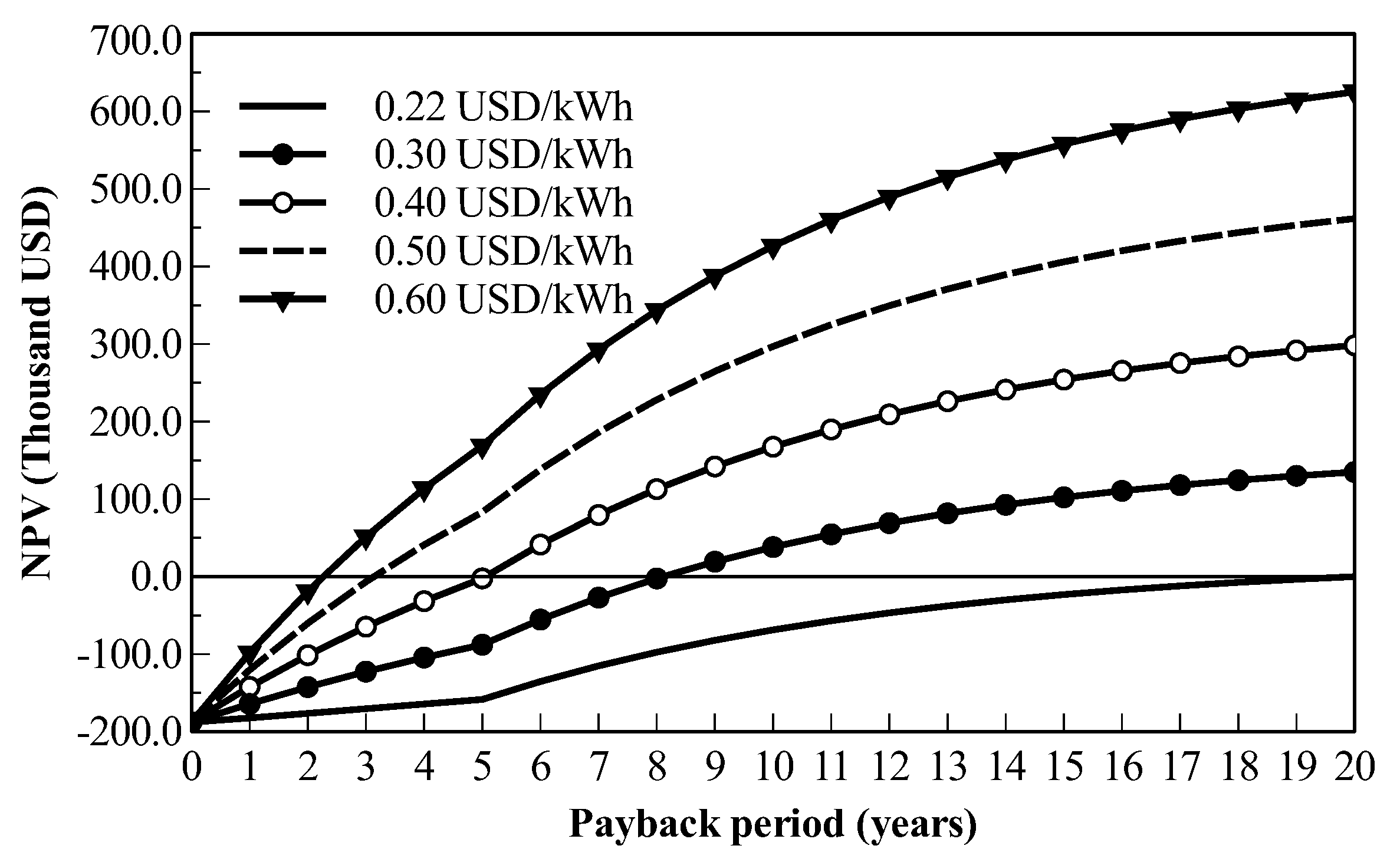
3.5. Net Present Value (NPV)

Since LCOE is considered as the average minimum cost at which electricity must be sold in order to break-even over the lifetime of the project, values in Table 7 consider a payback period of 20 years. Remark that LCOE allows to assess the performance of different ORC configurations, operating with different working fluids, under the same future scenario. However, to achieve a lower payback period, the selling price of energy must be higher than the calculated via LCOE. Figure 7 shows NPV for five values of selling price of energy. Results in Figure 7 corresponds to simple ORC operating with R1234ze(Z) at the highest heat source temperature and optimum net power output. Results for NPV indicate that a moderate increment in the selling price of energy (from 0.22 to 0.3 USD/kWh) leads to a reduction in the payback period from 20 to 8 years. Energy selling prices in the range 0.2–0.3 USD/kWh are not competitive compared to the average price of electricity for industrial users in the United States, which is between 0.05 and 0.2 USD/kWh, but are close to the average price of electricity for residential users, which is between 0.1 and 0.3 USD/kWh [49]. Nevertheless, in non interconnected areas, the electricity cost of new rooftop Solar Photovolaic (PV) systems ranges between 0.1 and 0.4 USD/kWh [50] and the cost of electricity in Concentrated Solar Power (CSP) via parabolic trough collectors, which is the most common and mature solar thermal power technology [51], is between 0.17 and 0.35 USD/kWh [52], showing that simple ORC with a selling price of energy of 0.3 USD/kWh could be a feasible option, depending on the profitability input parameters and taxes.

4. Conclusions

In this paper thermodynamic optimization and economic analysis of the dual pressure ORC is carried out to compare its performance and profitability with two common configurations: Simple and Regenerative ORC. In the optimization process pressure ratio and the minimum approach temperature in the evaporator are varied to maximize net power output and thermal efficiency independently. In the economic analysis LCOE and SIC are calculated to compare the different cycle configurations and the optimization results. As a distinguishing feature our study focuses on small-scale applications requiring power output of less than 45 kW. After presenting the results and identify trends, the following conclusions are established:

• Dual pressure ORC is the configuration that achieves the highest net power output at heat source temperatures below 130 °C. Dual pressure ORC is more attractive at heat source temperatures close to 100 °C. Above 130 °C, simple ORC with R1234ze(Z) develops the highest power output.
• From the thermal efficiency optimization, regenerative ORC with R1234ze(Z) is the combination with the maximum thermal efficiency. However, its net power output is rather low compared with R11234yf and R1234ze(E), which develop less thermal efficiency but higher net power output when thermal efficiency is optimized.
• Net power output and thermal efficiency optimization show different trends when they are optimized separately. However, LCOE values show that thermal efficiency optimization is less cost-effective than net power output optimization.
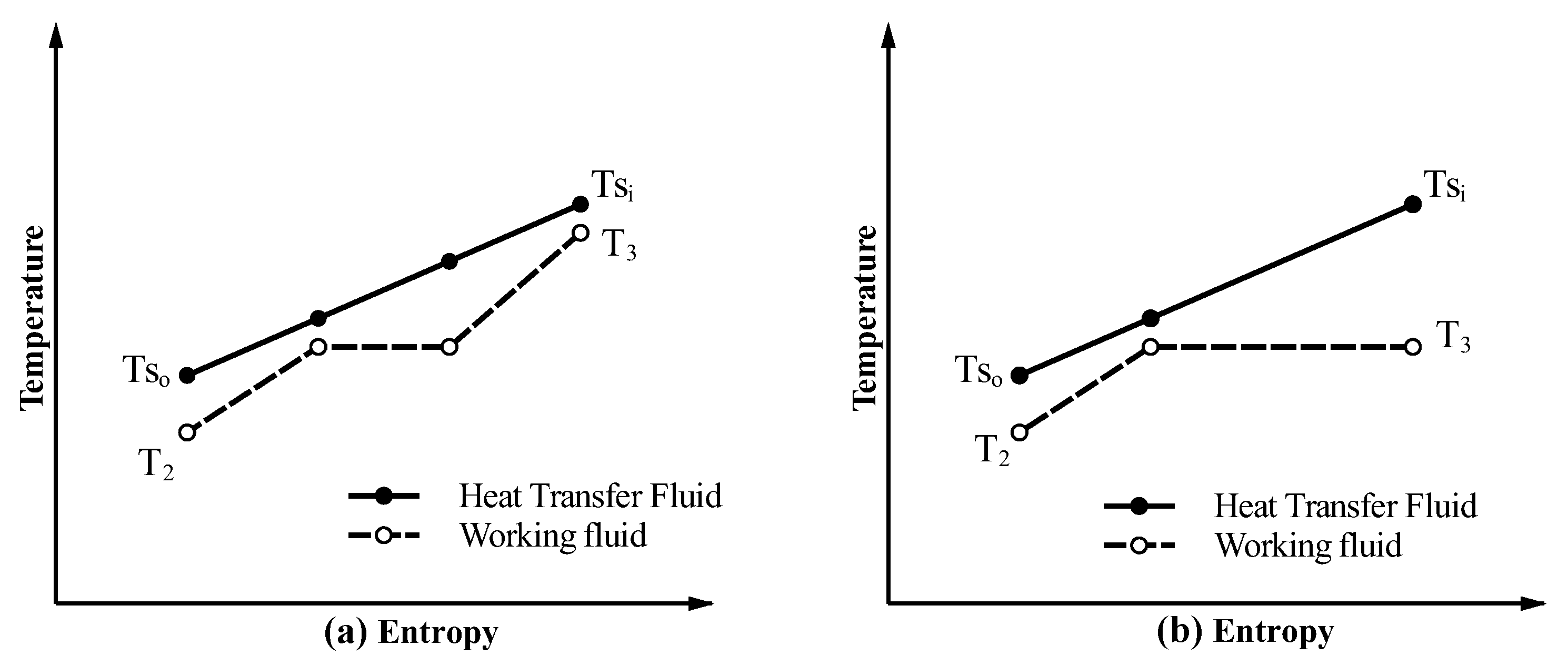
• There are higher exergy destruction and lower exergy efficiency rates when net power is optimized as compared to the case in which thermal efficiency is optimized. The inclusion of the regenerative heat exchanger reduces the exergy destruction and increases the exergy efficiency, but dual pressure ORC is the configuration with the lowest exergy efficiency and the highest exergy destruction, specially at higher temperatures, where the working fluid is superheated.
• According to the economic evaluation, LCOE and SIC values show that the conventional simple ORC is the most cost-effective among the studied cycle configurations when either net power or thermal efficiency is optimized, requiring a selling price of energy of 0.3 USD/kWh to obtain a payback period of 8 years. In addition, the working fluid R1234ze(Z) exhibits great potential for simple ORC when compared to conventional R245fa.

References

1. Cruz Virosa, I.; Filgueiras Sainz de Rozas, M.L.; Sorinas Gonzáles, L.; Cabello Eras, J.J.; Fernández Pérez, L. Gestión comparada del riesgo en el control de la contaminación atmosférica de Generadores de Vapor. Ingeniería Energética 2016, 37, 195–206. (In Spanish) [Google Scholar]
2. Eras, J.J.C.; Gutiérrez, A.S.; Lorenzo, D.G.; Martínez, J.B.C.; Hens, L.; Vandecasteele, C. Bridging universities and industry through cleaner production activities. Experiences from the Cleaner Production Center at the University of Cienfuegos, Cuba. J. Clean. Prod. 2015, 108, 873–882. [Google Scholar] [CrossRef]
3. Fontalvo, A.; Pinzon, H.; Duarte, J.; Bula, A.; Quiroga, A.G.; Padilla, R.V. Exergy analysis of a combined power and cooling cycle. Appl. Therm. Eng. 2013, 60, 164–171. [Google Scholar] [CrossRef]
4. Loni, R.; Kasaeian, A.; Mahian, O.; Sahin, A.Z.; Wongwises, S. Exergy analysis of a solar organic Rankine cycle with square prismatic cavity receiver. Int. J. Exergy 2017, 22, 103–124. [Google Scholar] [CrossRef]
5. Demirkaya, G.; Padilla, R.V.; Fontalvo, A.; Lake, M.; Lim, Y.Y. Thermal and Exergetic Analysis of the Goswami Cycle Integrated with Mid-Grade Heat Sources. Entropy 2017, 19, 416. [Google Scholar] [CrossRef]
6. Golzari, S.; Kasaeian, A.; Daviran, S.; Mahian, O.; Wongwises, S.; Sahin, A.Z. Second law analysis of an automotive air conditioning system using HFO-1234yf, an environmentally friendly refrigerant. Int. J. Refrig. 2017, 73, 134–143. [Google Scholar] [CrossRef]
7. Mahian, O.; Kianifar, A.; Heris, S.Z.; Wen, D.; Sahin, A.Z.; Wongwises, S. Nanofluids effects on the evaporation rate in a solar still equipped with a heat exchanger. Nano Energy 2017, 36, 134–155. [Google Scholar] [CrossRef]
8. Ormat Technologies Global Projects. Available online: http://www.ormat.com/global-project (accessed on 1 February 2017).
9. Quoilin, S.; Van Den Broek, M.; Declaye, S.; Dewallef, P.; Lemort, V. Techno-economic survey of Organic Rankine Cycle (ORC) systems. Renew. Sustain. Energy Rev. 2013, 22, 168–186. [Google Scholar] [CrossRef]
10. Turbodenl Products for Combined Heat and Power (CHP). Available online: http://www.turboden.eu/en/products/products-chp.php (accessed on 1 February 2017).
11. Turboden Solar Thermal Power Applications. Available online: http://www.turboden.eu/en/public/downloads/11-COM.P-6-rev.10%20-%20SOLAR%20ENGLISH.pdf (accessed on 1 February 2017).
12. White, M.; Sayma, A.I. Improving the economy-of-scale of small organic rankine cycle systems through appropriate working fluid selection. Appl. Energy 2016, 183, 1227–1239. [Google Scholar] [CrossRef]
13. Baral, S.; Kim, D.; Yun, E.; Kim, K.C. Experimental and thermoeconomic analysis of small-scale solar organic Rankine cycle (SORC) system. Entropy 2015, 17, 2039–2061. [Google Scholar] [CrossRef]
14. Peris, B.; Navarro-Esbri, J.; Moles, F.; Mota-Babiloni, A. Experimental study of an ORC (organic Rankine cycle) for low grade waste heat recovery in a ceramic industry. Energy 2015, 85, 534–542. [Google Scholar] [CrossRef]
15. Li, J.; Pei, G.; Li, Y.; Ji, J. Evaluation of external heat loss from a small-scale expander used in organic Rankine cycle. Appl. Therm. Eng. 2011, 31, 2694–2701. [Google Scholar] [CrossRef]
16. Lemort, V.; Quoilin, S.; Cuevas, C.; Lebrun, J. Testing and modeling a scroll expander integrated into an Organic Rankine Cycle. Appl. Therm. Eng. 2009, 29, 3094–3102. [Google Scholar] [CrossRef]
17. Gao, P.; Jiang, L.; Wang, L.; Wang, R.; Song, F. Simulation and experiments on an ORC system with different scroll expanders based on energy and exergy analysis. Appl. Therm. Eng. 2015, 75, 880–888. [Google Scholar] [CrossRef]
18. Wang, E.; Zhang, H.; Fan, B.; Ouyang, M.; Zhao, Y.; Mu, Q. Study of working fluid selection of organic Rankine cycle (ORC) for engine waste heat recovery. Energy 2011, 36, 3406–3418. [Google Scholar] [CrossRef]
19. Leibowitz, H.; Smith, I.; Stosic, N. Cost effective small scale ORC systems for power recovery from low grade heat sources. In Proceedings of the ASME 2006 International Mechanical Engineering Congress and Exposition, Chicago, IL, USA, 5–10 November 2006; pp. 521–527. [Google Scholar]
20. Ziviani, D.; Bell, I.; van den Broek, M.; De Paepe, M. Comprehensive Model of a Single-screw Expander for ORC-Systems. In Proceedings of the International Compressor Engineering Conference, Ghent, Belgium, 14–17 July 2014. [Google Scholar]
21. Yamamoto, T.; Furuhata, T.; Arai, N.; Mori, K. Design and testing of the organic Rankine cycle. Energy 2001, 26, 239–251. [Google Scholar] [CrossRef]
22. Kang, S.H. Design and experimental study of ORC (organic Rankine cycle) and radial turbine using R245fa working fluid. Energy 2012, 41, 514–524. [Google Scholar] [CrossRef]
23. Fiaschi, D.; Manfrida, G.; Maraschiello, F. Thermo-fluid dynamics preliminary design of turbo-expanders for ORC cycles. Appl. Energy 2012, 97, 601–608. [Google Scholar] [CrossRef]
24. Fiaschi, D.; Manfrida, G.; Maraschiello, F. Design and performance prediction of radial ORC turboexpanders. Appl. Energy 2015, 138, 517–532. [Google Scholar] [CrossRef]
25. Manente, G.; Lazzaretto, A.; Bonamico, E. Design guidelines for the choice between single and dual pressure layouts in organic Rankine cycle (ORC) systems. Energy 2017, 123, 413–431. [Google Scholar] [CrossRef]
26. Abadi, G.B.; Yun, E.; Kim, K.C. Experimental study of a 1 kw organic Rankine cycle with a zeotropic mixture of R245fa/R134a. Energy 2015, 93, 2363–2373. [Google Scholar] [CrossRef]
27. Li, T.; Zhang, Z.; Lu, J.; Yang, J.; Hu, Y. Two-stage evaporation strategy to improve system performance for organic Rankine cycle. Appl. Energy 2015, 150, 323–334. [Google Scholar] [CrossRef]
28. Lecompte, S.; Huisseune, H.; van den Broek, M.; Vanslambrouck, B.; De Paepe, M. Review of organic Rankine cycle (ORC) architectures for waste heat recovery. Renew. Sustain. Energy Rev. 2015, 47, 448–461. [Google Scholar] [CrossRef]
29. Abadi, G.B.; Kim, K.C. Investigation of organic Rankine cycles with zeotropic mixtures as a working fluid: Advantages and issues. Renew. Sustain. Energy Rev. 2017, 73, 1000–1013. [Google Scholar] [CrossRef]
30. Rahbar, K.; Mahmoud, S.; Al-Dadah, R.K.; Moazami, N.; Mirhadizadeh, S.A. Review of organic Rankine cycle for small-scale applications. Energy Convers. Manag. 2017, 134, 135–155. [Google Scholar] [CrossRef]
31. Lemmon, E.W.; Huber, M.L.; McLinden, M.O. NIST Standard Reference Database 23: Reference Fluid Thermodynamic and Transport Properties-REFPROP, Version 9.1.; Technical Report; National Institute of Standards and Technology: Gaithersburg, MD, USA, 2013. [Google Scholar]
32. European Union. Directive 2006/40/EC of the European Parliament and of the Council of 17 May 2006 relating to emissions from air-conditioning systems in motor vehicles and Amending Council Directive 70/156/EEC. Off. J. Eur. Union 2006, 1, 12–18. [Google Scholar]
33. Maizza, V.; Maizza, A. Working fluids in non-steady flows for waste energy recovery systems. Appl. Therm. Eng. 1996, 16, 579–590. [Google Scholar] [CrossRef]
34. Tchanche, B.F. Low Grade Heat Conversion into Power Using Small Scale Organic Rankine Cycles. Ph.D. Thesis, Agricultural University of Athens, Athens, Greece, 2011. [Google Scholar]
35. Moran, M.J.; Shapiro, H.N. Fundamentals of Engineering Thermodynamics, 5th ed.; John Wiley & Sons: Hoboken, NJ, USA, 2004. [Google Scholar]
36. Shah, R.K.; Sekulic, D.P. Fundamentals of Heat Exchanger Design; John Wiley & Sons: Hoboken, NJ, USA, 2003. [Google Scholar]
37. Turizo-Santos, J.; Barros-Ballesteros, O.; Fontalvo-Lascano, A.; Vasquez-Padilla, R.; Bula-Silvera, A. Experimental characterization of thermal hydraulic performance of louvered brazed plate fin heat exchangers. Rev. Fac. Ing. Univ. Antioquia 2015, 74, 108–116. [Google Scholar]
38. Sinnott, R.K. Chemical Engineering Design: SI Edition; Elsevier: Amsterdam, The Netherlands, 2009. [Google Scholar]
39. Huang, J.; Sheer, T.J.; Bailey-McEwan, M. Heat transfer and pressure drop in plate heat exchanger refrigerant evaporators. Int. J. Refrig. 2012, 35, 325–335. [Google Scholar] [CrossRef]
40. Yan, Y.Y.; Lio, H.C.; Lin, T.F. Condensation heat transfer and pressure drop of refrigerant R-134a in a plate heat exchanger. Int. J. Heat Mass Transf. 1999, 42, 993–1006. [Google Scholar] [CrossRef]
41. Bejan, A.; Tsatsaronis, G. Thermal Design and Optimization; John Wiley & Sons: Hoboken, NJ, USA, 1996. [Google Scholar]
42. Infinity Turbine Waste Heat to Power. Available online: http://www.infinityturbine.com/ (accessed on 1 February 2017).
43. Standard Xchange, Xylem Brazepak—Stainless Steel/copper Brazed Plate. Available online: http://www.standard-xchange.com/ (accessed on 1 February 2017).
44. Lukawski, M. Design and Optimization of Standardized Organic Rankine Cycle Power Plant for European Conditions. Master’s Thesis, School for Renewable Energy Science, Akureyri, Iceland, December 2010. [Google Scholar]
45. Perry, R.H.; Green, D.W. Perry’s Chemical Engineers’ Handbook; McGraw-Hill: New York, NY, USA, 2008. [Google Scholar]
46. Loni, R.; Kasaeian, A.B.; Mahian, O.; Sahin, A.Z. Thermodynamic analysis of an organic rankine cycle using a tubular solar cavity receiver. Energy Convers. Manag. 2016, 127, 494–503. [Google Scholar] [CrossRef]
47. Galindo, J.; Climent, H.; Dolz, V.; Royo-Pascual, L. Multi-objective optimization of a bottoming Organic Rankine Cycle (ORC) of gasoline engine using swash-plate expander. Energy Convers. Manag. 2016, 126, 1054–1065. [Google Scholar] [CrossRef]
48. Quoilin, S.; Declaye, S.; Tchanche, B.; Lemort, V. Thermo-economic optimization of waste heat recovery Organic Rankine Cycles. Appl. Therm. Eng. 2011, 31, 2885–2893. [Google Scholar] [CrossRef]
49. Electric Power Monthly. Available online: https://www.eia.gov/electricity/monthly/epm_table_grapher.php?t=epmt_5_6_a (accessed on 25 August 2017).
50. Technology Roadmap: Solar Photovoltaic Energy, 2014 edition. Available online: https://www.iea.org/publications/freepublications/publication/TechnologyRoadmapSolarPhotovoltaicEnergy_2014edition.pdf (accessed on 25 August 2017).
51. Padilla, R.V.; Fontalvo, A.; Demirkaya, G.; Martinez, A.; Quiroga, A.G. Exergy analysis of parabolic trough solar receiver. Appl. Therm. Eng. 2014, 67, 579–586. [Google Scholar] [CrossRef]
52. Renewable Power Generation Costs in 2014. Available online: https://www.irena.org/DocumentDownloads/Publications/IRENA_RE_Power_Costs_2014_report.pdf (accessed on 25 August 2017).
Figure 1. ORC cycle configurations. (a) simple ORC; (b) regenerative ORC; and (c) dual pressure ORC.
Entropy 19 00476 g001
Figure 2. Minimum approach temperature in the evaporator. (a) Superheated vapor. (b) Saturated vapor.
Entropy 19 00476 g002
Figure 3. Sequence of the simulation process.
Entropy 19 00476 g003
Figure 4. Cost structure for the economic analysis. AFUDC: Allowance of Funds Used During Construction.
Entropy 19 00476 g004
Figure 5. Net power output and Thermal Efficiency optimization for different heat source temperatures. Working fluids: R1234yf, R1234ze(E) and R1234ze(Z). Cycle configurations: (a) Simple ORC. (b) Regenerative ORC and (c) Dual pressure ORC. NPO = Net Power Optimization. TEO = Thermal Efficiency Optimization.
Entropy 19 00476 g005
Figure 6. Exergy Efficiency vs. Heat source temperature. Working fluids: R1234yf, R1234ze(E) and R1234ze(Z). Cycle configurations: (a) Net power optimization. (b) Thermal efficiency optimization.
Entropy 19 00476 g006
Figure 7. Net Present Value (NPV) vs. payback period for net power optimization. Heat source temperature: 200 °C. Cycle: simple ORC. Working fluid: R1234ze(Z).
Entropy 19 00476 g007