Entropy Ensemble Filter: A Modified Bootstrap Aggregating (Bagging) Procedure to Improve Efficiency in Ensemble Model Simulation


Department of Civil Engineering, University of British Columbia, Vancouver, BC V6T 1Z4, Canada
*
Author to whom correspondence should be addressed.
Entropy 2017, 19(10), 520; https://doi.org/10.3390/e19100520
Submission received: 11 August 2017
/
Revised: 12 September 2017
/
Accepted: 26 September 2017
/
Published: 28 September 2017
(This article belongs to the Special Issue Information Theory in Machine Learning and Data Science)
Abstract
:Over the past two decades, the Bootstrap AGGregatING (bagging) method has been widely used for improving simulation. The computational cost of this method scales with the size of the ensemble, but excessively reducing the ensemble size comes at the cost of reduced predictive performance. The novel procedure proposed in this study is the Entropy Ensemble Filter (EEF), which uses the most informative training data sets in the ensemble rather than all ensemble members created by the bagging method. The results of this study indicate efficiency of the proposed method in application to synthetic data simulation on a sinusoidal signal, a sawtooth signal, and a composite signal. The EEF method can reduce the computational time of simulation by around 50% on average while maintaining predictive performance at the same level of the conventional method, where all of the ensemble models are used for simulation. The analysis of the error gradient (root mean square error of ensemble averages) shows that using the 40% most informative ensemble members of the set initially defined by the user appears to be most effective.
1. Introduction
Machine learning is one of the key components of computational intelligence and its main objective is to use computational methods to become more accurate in predicting outcomes without being explicitly programmed. Machine learning has a wide spectrum of applications in different science disciplines [1,2,3,4,5,6,7,8,9]. Advanced computational methods, including artificial neural networks (ANN), process input data in the context of previous training history on a defined sample database to produce relevant output [7]. To avoid negative effects of over-fitting, an ensemble of models is sometimes used in prediction [10]. In machine learning jargon, an ensemble of models is often referred to as a committee [5]. Bagging (abbreviated from Bootstrap AGGregatING) [11] developed from the idea of bootstrapping [12,13] in statistics. Under bootstrap resampling, data are drawn randomly from a dataset to form a new training dataset, which has the same number of data points as the original dataset. In committee machines, bagging is widely used for its simplicity and efficiency in enhancing the prediction power of individual models, also called experts [11]. Applications have spanned a wide range of fields. Zhu et al. [14] applied the bagging method to the forecasting of tropical cyclone tracks over the South China Sea. Fraz et al. [15] used an ensemble system of bagged and boosted decision trees to retinal blood vessel segmentation. Brenning [16] investigates the performance of bagging in spatial prediction models for landslide hazards. Dietterich [17] compared the effectiveness of bagging, boosting, and randomization methods for constructing ensembles of decision trees. A recurring question in these previous works was: how to choose the ensemble of training data sets for tuning the weights in machine learning? The computational cost of ensemble-based methods scales with the size of the ensemble, but excessively reducing the ensemble size comes at the cost of reduced predictive performance. The choice of ensemble size was often based on the size of input data and available computational power, which can become a limiting factor for larger datasets and models.
This paper presents the Entropy Ensemble Filter (EEF) as a method to reduce ensemble size without significantly deteriorating prediction performance. Conversely, we show that for small ensemble sizes, selecting for high entropy training sets can improve performance at the same computational burden. Entropy can be defined as uncertainty of a random variable or, conversely, the information that samples of that random variable provide. It is also known as the self-information of a random variable [18]. In this work, entropy is used as a measure of information content for each bootstrap resample of the dataset. The method selects high entropy bootstrap samples for ensemble model training, aiming to maximize information content in the selected ensemble. We applied our proposed method on a simulation of synthetic data with the ANN machine learning technique. The performance results of our proposed method are analyzed in comparison with those obtained by the conventional method when all ensemble members or a random subset are used for training.
2. Methods: Entropy Ensemble Filter
The philosophy of the EEF method is rooted in using self-information of a random variable, defined by Shannon’s information theory [19] for selection, to provide direction in the inherent randomness of ensemble models which are created by bootstrapping. In previous work, a weighting of model-generated ensemble members based on relative entropy was used [20] to reflect additional information available after ensemble generation. In this work, the focus is on selecting an ensemble of training datasets before ensemble model tuning (training of the ANNs). It is our hypothesis that if an ensemble of ANN models or any other machine learning technique uses the most informative ensemble members for training purpose rather than all bootstrapped ensemble members, it could reduce the computational time substantially without negatively affecting the performance of simulation. We discuss the EEF algorithm based on Shannon information theory. Shannon quantifies information by calculating the smallest possible number of bits, on average, to communicate outcomes of a random variable, e.g., per symbol in a message (here, symbols represent bins in a probability mass function which are defined with respect to input data resolution) [18,19,21,22]. The Shannon entropy H, in units of bits (per symbol), of ensemble member m in the bootstrapped dataset (generated from step 1, Algorithm 1), is given by:
where pyk is the probability of occurrence, within ensemble member m, with values according to random variable Y, of the kth possible value of the variable (K is a total number of discrete values Y can take, i.e., the number of bins in discretization). This equation gives the entropy in the units of “bits” because it uses a logarithm of base 2. Algorithm 1 illustrates the workflow of the EEF method. The EEF method can assess and cluster the ensemble members to provide the most informative ones for training, selected from the initially generated ensemble. Since model training is by far the most computationally expensive part of the procedure, overall computation time is roughly linear with the number of retained ensemble members, potentially leading to significant savings.
| Algorithm 1. Entropy Ensemble Filter | ||
| Begin | Comment | |
| 1 | Initialize the procedure of bagging | |
| Generate M new training datasets from input data using bootstrapping (M committee members) | M: Initially user defines the ensemble size | |
| 2 | Estimate the entropy of each ensemble member | |
| Hm ← Equation (1) | ||
| 3 | Find the top L ensemble member with maximum entropy | Determine L based on computational constraints. Alternative choice is to use 40% of members based on the analysis of error gradient (L = 0.4M) |
| Sort the ensemble members and find the L most informative ones | ||
| 4 | Set up neural networks or other machine learning techniques | |
| Use the most informative ensemble L members rather than M ensemble members for training or calibrating the weights inside the model | ||
| 5 | Use ensemble averages instead of individual ensemble models | |
| The rationale for using ensemble averages is that the expected error of the ensemble average is less than or equal to the average expected error of the individual models in the ensemble | ||
| End | ||
3. Application: Synthetic Data Simulation
In this section, the EEF method is tested by using synthetic data and artificial neural networks. Le et al. [23] note that “the deep learning community has reported remarkable results taking the synthetic data to train artificial neural networks”. We use artificial signals that we corrupt with noise before model training to examine the model’s capability to capture the essence of the signal from the noisy signal. In this study, a sinusoidal signal, a non-sinusoidal periodic waveform (sawtooth wave), and a nonperiodic composite signal have been used to create signals that we interpret as a true underlying process (target signal) we wish to simulate. However, these signals are not directly observable for model training, but corrupted by noise that represents, e.g., measurement error or unknown external influences. These target signals are chosen because of the following reasons:
- Sinusoids are ubiquitous in physics because many physical systems that resonate or oscillate produce quasi-sinusoidal motion.
- The performance of the method for simulation of a non-sinusoidal waveform was tested on a sawtooth signal, a classical geometric waveform.
- A composite signal has been used to test the performance of the method for simulation of nonperiodic signals. The signal has been composed of upward steps followed by exponential decay functions, which resemble typical behaviour for river flow response to rainfall events.
Procedure
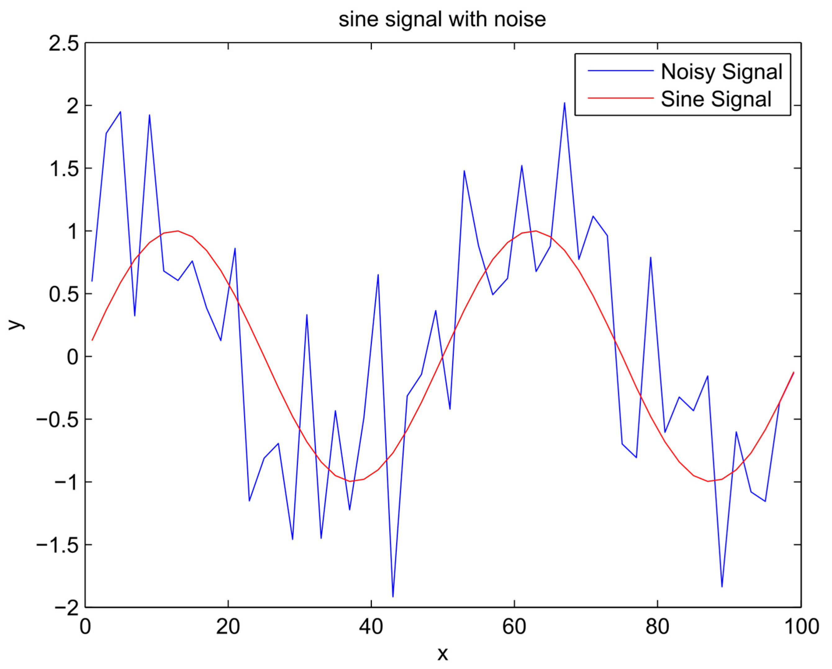
First, random noise with a normal distribution was added to the known sinusoidal, sawtooth, and composite signals (Equations (2)–(4) respectively) to make the noisy signal (Equation (5)) presented in Figure 1, Figure 2 and Figure 3. The noisy signal was used as an input in the bagging procedure to generate an ensemble of input datasets, referred to as ensemble members. Following the steps described in Algorithm 1, the chosen members by the EEF method are used for training ANN’s and subsequently generating the simulation result for each member (Equation (6)).
The RMSE of the ensemble average in Equation (8) shown for the EEF method is calculated with respect to the original target signals y (Equations (2)–(4)).
The entropy calculations for each ensemble member are performed in a discretized space, where the signals are processed using 10 bins of equal bin-size arranged between the signal’s minimum and maximum values. These bin sizes were chosen to strike a balance between being fine enough to capture the distribution of the values in the time series, while being coarse enough so that enough data points are available per bin to have a representative histogram. The entropies of all training datasets in the ensemble are then calculated by Shannon entropy equation (Equation (1)). Since entropy is calculated empirically, the method can be applied regardless of the data distribution type. The index of the highest entropy ensemble member found is used to determine the new ensemble size (see Appendix A). Then, the ensemble of training data sets are filtered, and only the top highest entropy training data sets are retained. ANN models were then trained on all bootstrapped noisy data sets retained in the ensemble, and on all original ensemble members for reference. In the experiments, the ANN that was used was a feed-forward multilayer perceptron model (by using a hyperbolic tangent activation function) with one input and output layer (the bootstrapped datasets), and 10, 50, and 20 hidden neurons. These were fitted to the bootstrapped noisy sinusoidal, sawtooth, and composite signals, respectively, using the early stopping procedure. For each ensemble, the predictions of the ANNs were averaged to yield an ensemble prediction. The distribution of the ensemble predictions is not forced to any parametric form, and, in general, bagging and our proposed modification are not sensitive to distribution type. The predictions were evaluated by calculating RMSE against the target signal, i.e., the synthetic data before the corruption by noise. Note that the true signal was not available for the ANN during training.
4. Results and Analysis
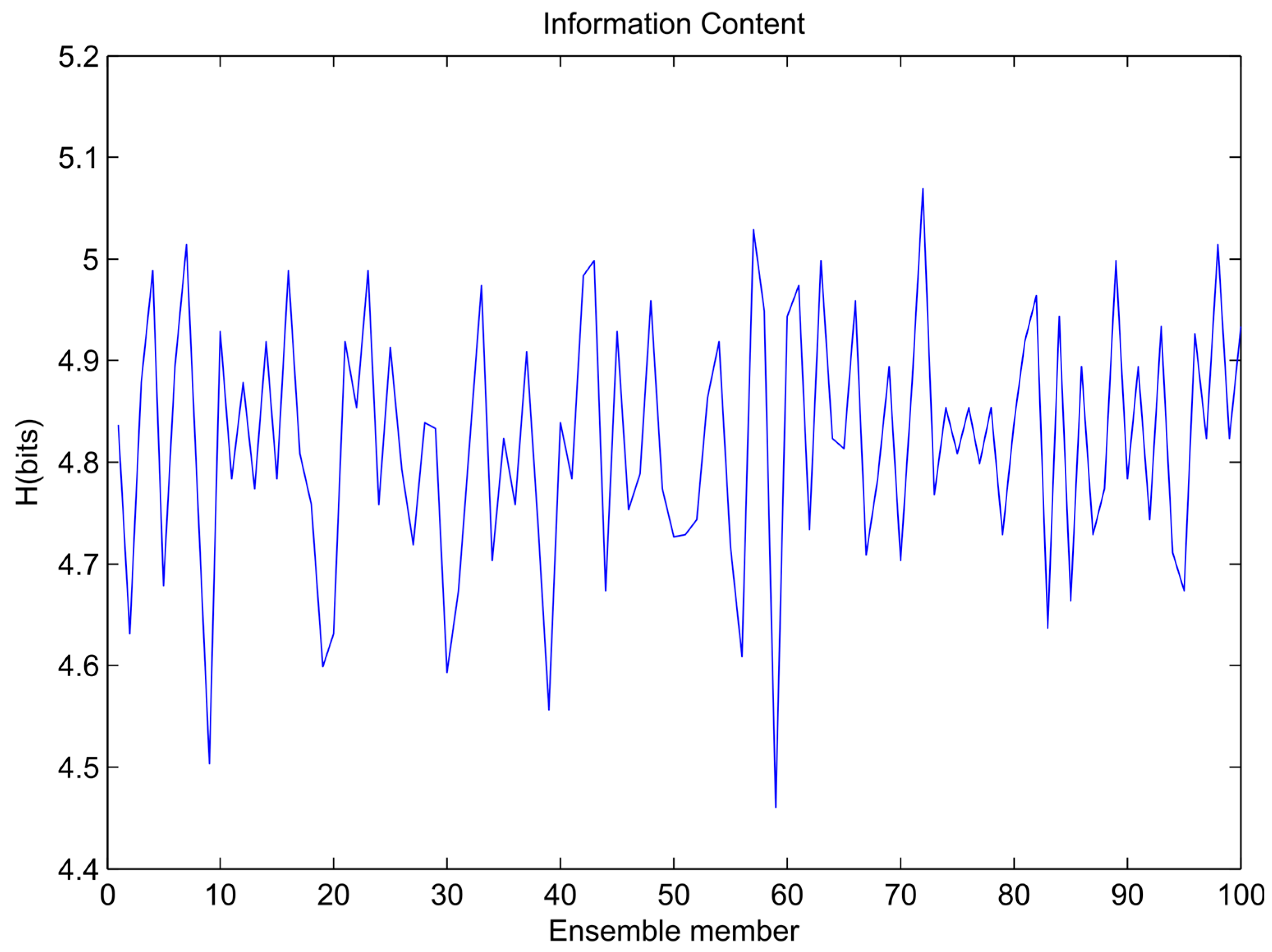
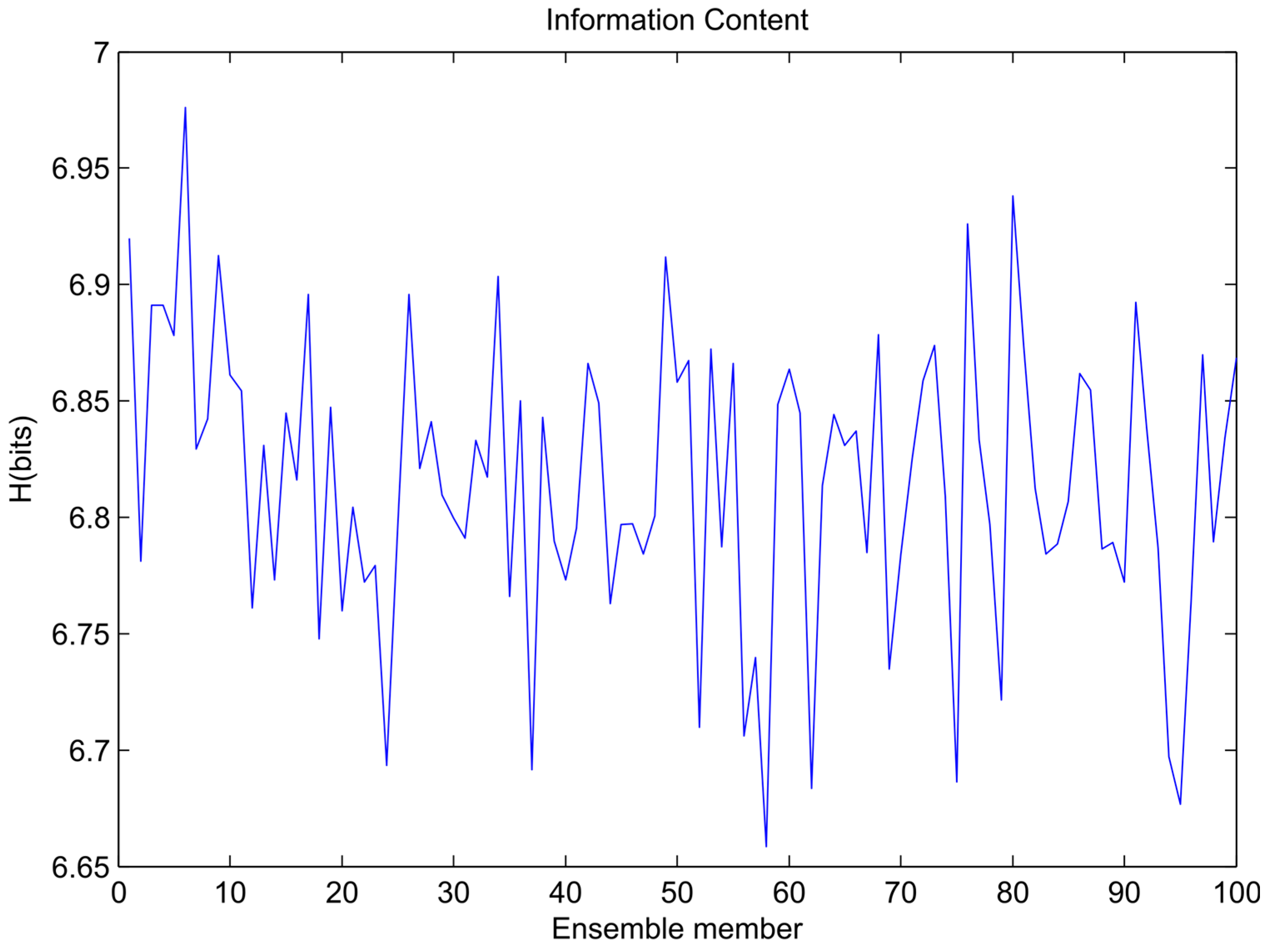
The variations of information content for each ensemble member training data set for the sinusoidal signal, sawtooth wave, and composite signal are shown in Figure 4, Figure 5 and Figure 6, respectively. In the figures it is visible that the bootstrapping leads to significant variability in the training dataset entropies.
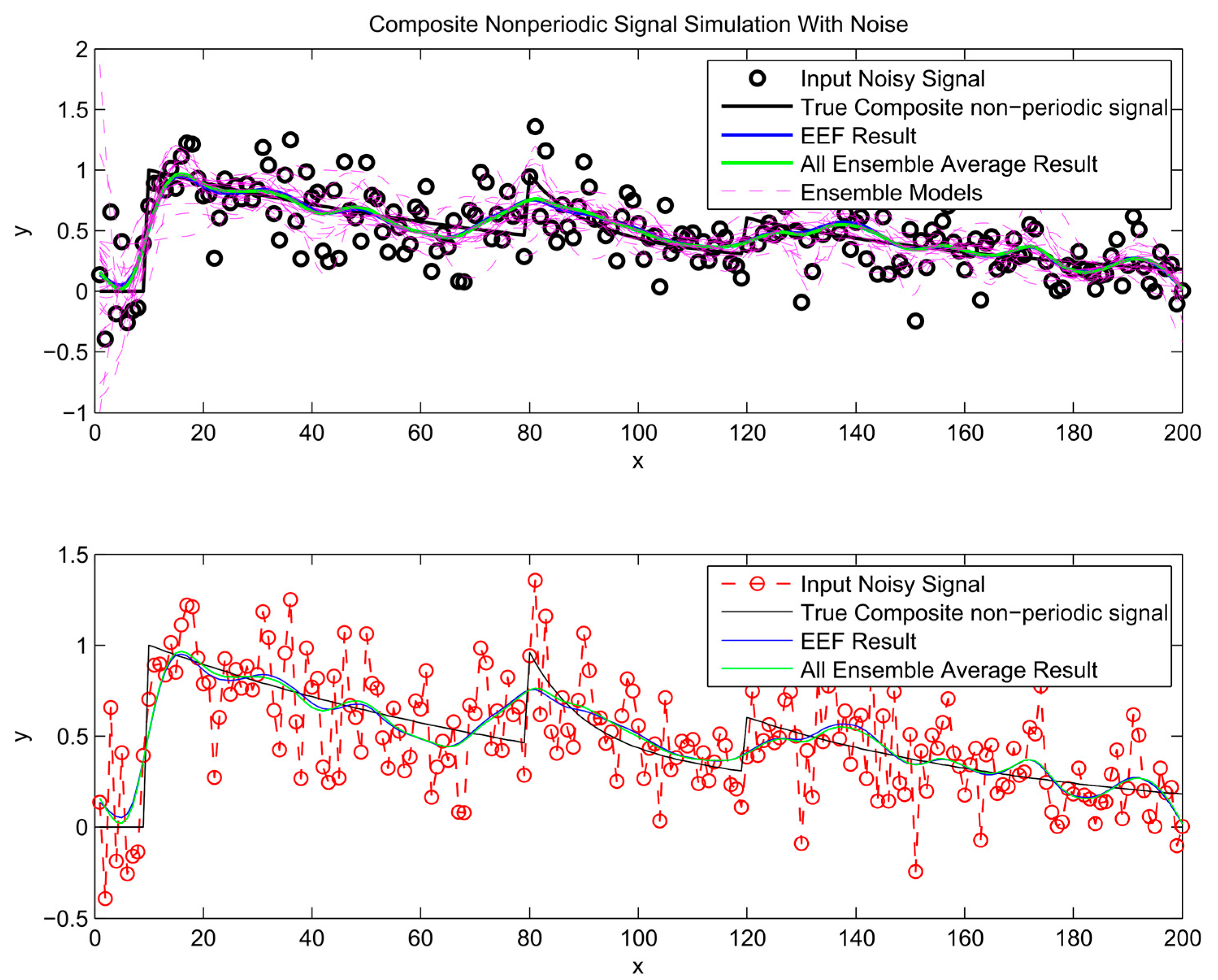
After the most informative ensemble members are chosen to train ANNs and their outputs have been processed through ensemble averaging, the predictions are plotted in Figure 7, Figure 8 and Figure 9. For comparison, the conventional bagging method, based on all ensemble members, is used to train a separate ensemble of neural networks. The prediction from these ensemble averages is included in the same figures. As illustrated in Figure 7, Figure 8 and Figure 9, the simulation results of using all ensemble members and the chosen ones by the EEF method closely resemble each other, which indicates that filtering the ensemble models could be a reliable method.
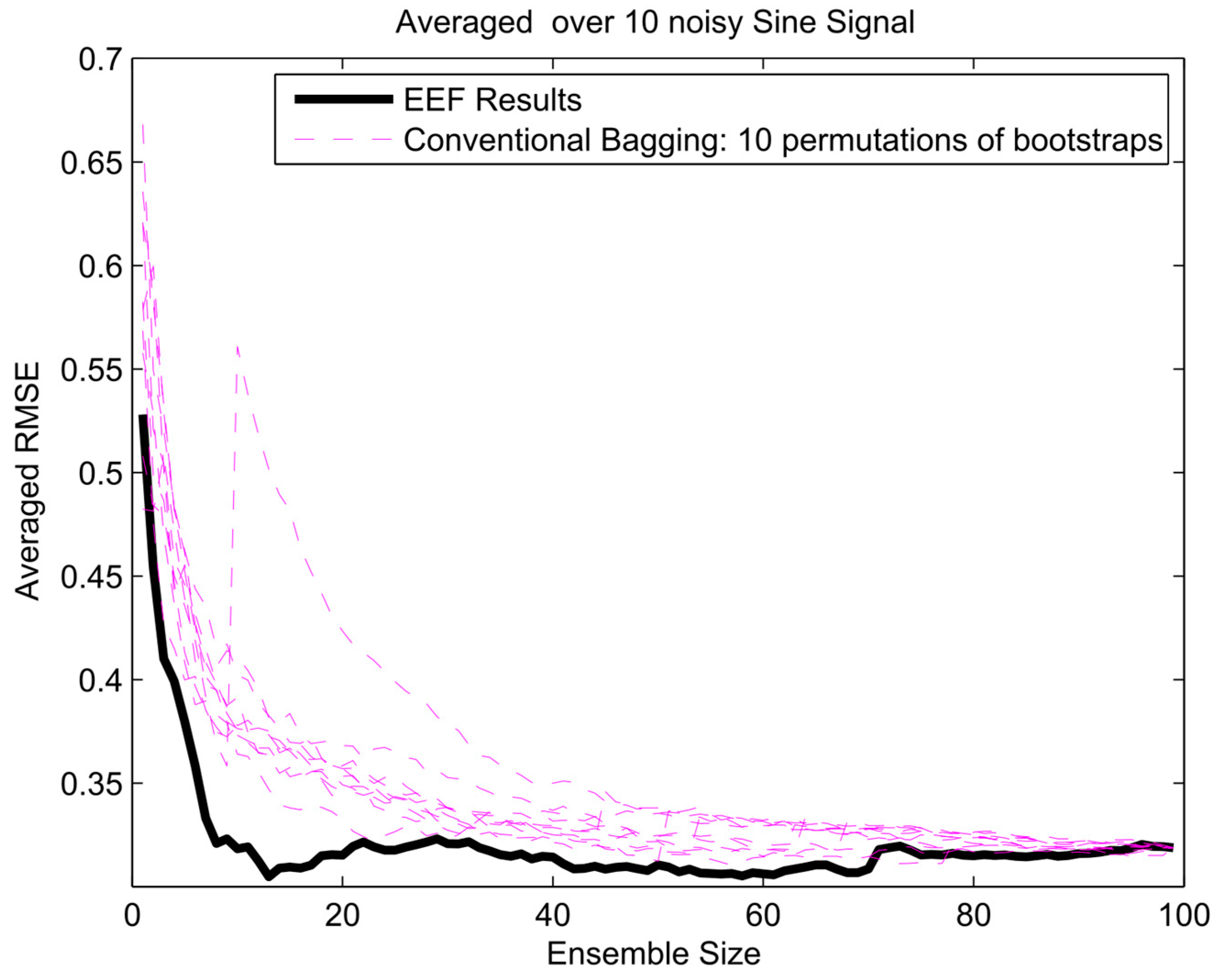
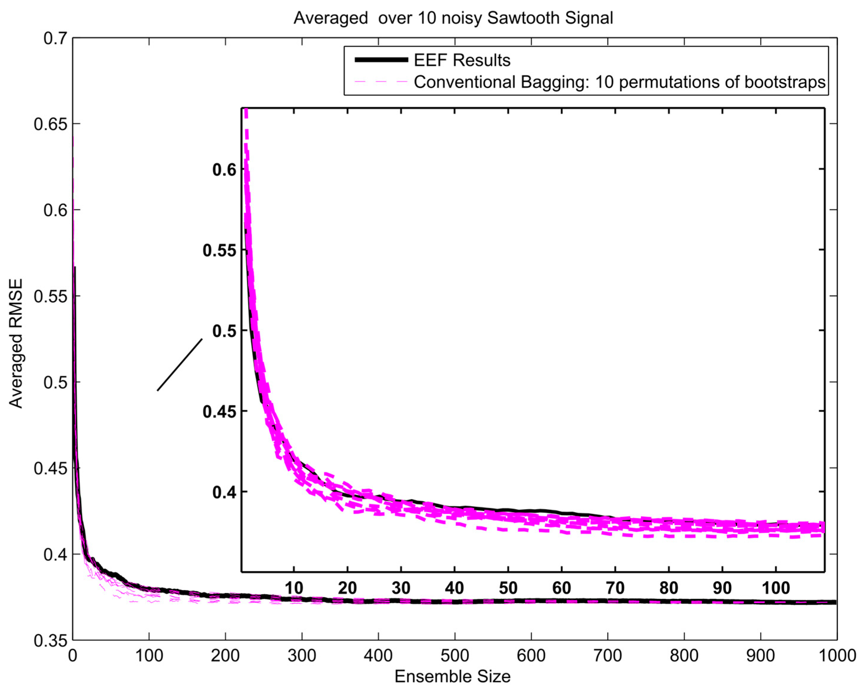
To get insight in the trade-off between ensemble size (i.e., computation time) and accuracy in terms of RMSE, analysis of the error gradient with growing ensemble size was conducted. In this analysis, the decrease in error was compared between using the EEF method and conventional bagging with increasing ensemble size. To filter out some of the inherent randomness from the results, the whole process was repeated ten times with different realizations of the random noise, and resulting RMSEs were averaged over these 10 realizations. The error gradient shows the effect of varying the final ensemble size after selection. However, also, the initial ensemble size plays a role in the prediction accuracy, since selecting from a larger initial pool of ensemble members means higher entropy values in the selection. In current practice, the user will decide on how many ensemble models are needed for training and tuning the weights in machine learning. Therefore, we show the results of error gradient analysis for 100 and 1000 initial bootstrapping in Figure 10, Figure 11 and Figure 12 and Figure 13, Figure 14 and Figure 15, respectively. The idea of ranking the ensemble by the EEF method and subsequently using it for machine learning shows its advantages in Figure 10 and Figure 13, for the sinusoidal signal. For the other signals, the advantages are mostly in the smallest ensemble sizes, visible in Figure 10, Figure 11, Figure 12, Figure 13, Figure 14 and Figure 15. The results show that using the 40% most informative ensemble members of the set initially defined by the user appears to be most effective.
An upwards jump in RMSE, such as seen for the conventional bagging in Figure 10 and Figure 13, indicates that an ensemble member (training data set) was picked that led to an ANN that does not perform well in prediction, deteriorating the ensemble average when added to the ensemble. The effect of adding such an ensemble member will be larger when the selected ensemble is still small in size, since the relative weight of the new member in the average will be higher. In the entropy-based ordering of the EEF, those ensemble members would also be picked eventually, but generally later in the sequence, when the effect on the total ensemble is small enough not to cause an important upward jump in RMSE. Since the EEF reduces the ensemble size, in many cases some of the poorly performing members will be eliminated from the ensemble. In the limit of using the full ensemble, the EEF and the conventional method converge upon each other (as seen at the extreme right of Figure 10, Figure 11, Figure 12, Figure 13, Figure 14 and Figure 15), since the full ensembles are identical. The fact that those jumps are not displayed in the EEF results indicates that these poorly performing ANNs are not among the ones trained on the top highest entropy training data sets. These are the ones that would typically be retained by the EEF method.
Furthermore, the EEF method has been tested with a different initial number of committee members illustrated in Table A1, Table A2 and Table A3 (see Appendix A). The results of the sinusoidal signal, sawtooth wave, and composite signal simulation indicate that the EEF method can improve the simulation error 3% on average for a sinusoidal signal, and relatively maintain error performance at the same level for sawtooth wave and composite signal. More importantly, empirical testing showed that it can reduce the simulation time by 54%, 56%, and 45% on average, respectively.
Protection against Overfitting
There are several layers in the procedure that offer protection against overfitting. Firstly, it is important to note that the entire prediction procedure never sees the original data set that is tested against, since only the noise-corrupted version of the data is used for training; however, the final evaluation of performance is against the non-noisy original data set.
Secondly, for both compared methods, the individual ensemble member ANNs are trained on bootstraps of these noise-corrupted data. For each individual data set in the selected ensemble, the ANN training uses the standard and well-tested early stopping (also known as stopped training) procedure to prevent overfitting. In this procedure, the data is divided in training and validation data and training continues until validation performance starts to deteriorate [5].
Thirdly, the bagging procedure adds another layer of protection against overfitting where the outcomes of several fitted models are averaged, reducing reliance on one single model. As can be seen in Figure 10, Figure 11, Figure 12, Figure 13, Figure 14 and Figure 15, larger ensemble sizes improve prediction up to a certain ensemble size. Therefore, a trade-off between accuracy and ensemble size exists for smaller ensembles. The EEF method provides a way to reduce ensemble size (and computational cost) with smaller decrease in performance, or, conversely, improve performance for fixed small ensemble sizes. In that sense, the EEF method is a Pareto improvement over the conventional method. The EEF selects ensemble members before any model is trained and therefore does not have access to the original signal or predictive performance. Summarizing, the EEF does not increase overfitting issues compared to conventional bagging, which already has safeguards in place at different levels.
5. Conclusions
In this article, we introduced a novel procedure to assess and cluster ensemble members for bootstrap aggregating (bagging). Fundamentally, we assert that the EEF method can reduce the computational time of simulation very substantially while maintaining error performance at the same level of the conventional method, where all of the ensemble models used for simulation. The idea of ranking and selecting the ensemble with the EEF method and subsequently using them for machine learning shows its advantages in Figure 10 and Figure 13. Figure 10, Figure 11, Figure 12, Figure 13, Figure 14 and Figure 15 show a clear effect of ensemble size on prediction quality for the smaller ensemble sizes. The positive effects of using the EEF method are most pronounced in the smallest ensemble sizes. The EEF method can be useful to meet the computational power constraints for the continual arrival of new data, which necessitates frequent model updating in atmospheric science. Peng et al. [24] note that computational expense is one of the difficulties in air quality forecasting. Although the results of this study indicated the efficiency of the proposed framework in application to synthetic data simulation, further evaluations of the proposed framework are still necessary, especially in applications to data assimilation problems with real data and numerous observations.
Acknowledgments
This research was supported with funding from Hossein Foroozand’s NSERC CGS M award and Steven V. Weijs’s NSERC discovery grant.
Author Contributions
Hossein Foroozand and Steven V. Weijs designed the method and experiments; Hossein Foroozand and Steven V. Weijs performed the experiments; Hossein Foroozand and Steven V. Weijs wrote the paper.
Conflicts of Interest
The authors declare no conflict of interest.
Appendix A. Results of EFF Method for Three Different Signals

Table A1.
Sinusoidal signal outputs of the EEF method for different initial committee members.
| All Ensemble | EEF Ensemble | Run Time EEF Ensemble (s) | Run Time All Ensemble (s) | RMSE EEF Ensemble | RMSE All Ensemble | Average % of Saving Time | Average Rate of Change in Error |
|---|---|---|---|---|---|---|---|
| 100 | 56 | 14.7 | 25.0 | 0.374 | 0.361 | 0.46 | 0.05 |
| 100 | 94 | 23.0 | 24.0 | 0.372 | 0.375 | ||
| 100 | 23 | 6.0 | 24.3 | 0.361 | 0.400 | ||
| 100 | 55 | 14.0 | 23.7 | 0.367 | 0.380 | ||
| 100 | 86 | 21.0 | 24.6 | 0.340 | 0.395 | ||
| 100 | 44 | 11.0 | 24.6 | 0.364 | 0.397 | ||
| 100 | 35 | 8.5 | 26.3 | 0.342 | 0.377 | ||
| 100 | 21 | 4.6 | 25.1 | 0.362 | 0.389 | ||
| 100 | 52 | 11.8 | 25.1 | 0.357 | 0.380 | ||
| 100 | 83 | 19.8 | 24.9 | 0.386 | 0.385 | ||
| 200 | 151 | 40.7 | 57.4 | 0.349 | 0.398 | 0.56 | 0.04 |
| 200 | 54 | 13.4 | 48.8 | 0.374 | 0.375 | ||
| 200 | 103 | 23.7 | 47.6 | 0.340 | 0.376 | ||
| 200 | 97 | 22.3 | 49.4 | 0.355 | 0.371 | ||
| 200 | 166 | 39.1 | 47.7 | 0.374 | 0.369 | ||
| 200 | 61 | 15.4 | 52.5 | 0.401 | 0.411 | ||
| 200 | 28 | 6.9 | 46.8 | 0.389 | 0.387 | ||
| 200 | 106 | 23.8 | 49.3 | 0.363 | 0.366 | ||
| 200 | 69 | 16.0 | 47.6 | 0.383 | 0.394 | ||
| 200 | 86 | 19.4 | 48.1 | 0.381 | 0.404 | ||
| 1000 | 246 | 62.1 | 250.4 | 0.379 | 0.383 | 0.62 | 0.01 |
| 1000 | 647 | 161.7 | 257.1 | 0.371 | 0.368 | ||
| 1000 | 373 | 91.2 | 246.7 | 0.369 | 0.388 | ||
| 1000 | 413 | 100.9 | 251.3 | 0.363 | 0.374 | ||
| 1000 | 395 | 98.0 | 248.7 | 0.391 | 0.388 | ||
| 1000 | 624 | 156.0 | 251.1 | 0.381 | 0.382 | ||
| 1000 | 91 | 21.8 | 248.8 | 0.378 | 0.382 | ||
| 1000 | 6 | 1.4 | 250.2 | 0.378 | 0.384 | ||
| 1000 | 627 | 153.7 | 249.2 | 0.373 | 0.379 |
Table A2.
Sawtooth wave outputs of the EEF method for different initial committee members.
| All Ensemble | EEF Ensemble | Run Time EEF Ensemble | Run Time All Ensemble | RMSE EEF Ensemble | RMSE All Ensemble | Average % of Saving Time | Average Rate of Change in Error |
|---|---|---|---|---|---|---|---|
| 100 | 40 | 15.9 | 34.9 | 0.371 | 0.343 | 0.62 | −0.012 |
| 100 | 38 | 13.1 | 35.9 | 0.340 | 0.353 | ||
| 100 | 43 | 15.3 | 33.1 | 0.351 | 0.358 | ||
| 100 | 61 | 21.3 | 33.3 | 0.354 | 0.341 | ||
| 100 | 93 | 29.7 | 30.2 | 0.342 | 0.351 | ||
| 100 | 9 | 3.1 | 31.1 | 0.338 | 0.354 | ||
| 100 | 14 | 4.6 | 34.1 | 0.341 | 0.348 | ||
| 100 | 37 | 11.8 | 33.0 | 0.340 | 0.349 | ||
| 100 | 16 | 4.8 | 32.5 | 0.337 | 0.349 | ||
| 100 | 16 | 5.7 | 34.2 | 0.342 | 0.353 | ||
| 200 | 144 | 49.1 | 64.0 | 0.351 | 0.349 | 0.57 | −0.001 |
| 200 | 125 | 42.0 | 67.0 | 0.347 | 0.357 | ||
| 200 | 60 | 18.2 | 64.5 | 0.347 | 0.341 | ||
| 200 | 68 | 20.6 | 69.0 | 0.353 | 0.349 | ||
| 200 | 64 | 20.3 | 70.8 | 0.352 | 0.349 | ||
| 200 | 84 | 27.9 | 69.2 | 0.351 | 0.350 | ||
| 200 | 109 | 37.3 | 66.8 | 0.343 | 0.351 | ||
| 200 | 6 | 2.4 | 73.7 | 0.341 | 0.344 | ||
| 200 | 73 | 25.3 | 69.4 | 0.349 | 0.348 | ||
| 200 | 148 | 47.9 | 70.4 | 0.345 | 0.344 | ||
| 1000 | 861 | 278.5 | 312.6 | 0.346 | 0.342 | 0.50 | −0.004 |
| 1000 | 409 | 122.1 | 308.2 | 0.347 | 0.346 | ||
| 1000 | 142 | 41.0 | 313.3 | 0.344 | 0.345 | ||
| 1000 | 285 | 88.0 | 320.7 | 0.348 | 0.347 | ||
| 1000 | 511 | 154.8 | 313.4 | 0.347 | 0.343 | ||
| 1000 | 282 | 89.0 | 310.2 | 0.347 | 0.343 | ||
| 1000 | 743 | 222.5 | 311.5 | 0.343 | 0.343 | ||
| 1000 | 689 | 214.4 | 316.1 | 0.344 | 0.346 | ||
| 1000 | 948 | 306.1 | 320.5 | 0.346 | 0.344 |
Table A3.
Composite signal outputs of the EEF method for different initial committee members.
| All Ensemble | EEF Ensemble | Run Time EEF Ensemble | Run Time All Ensemble | RMSE EEF Ensemble | RMSE All Ensemble | Average % of Saving Time | Average Rate of Change in Error |
|---|---|---|---|---|---|---|---|
| 100 | 91 | 28.6 | 34.3 | 0.09 | 0.089 | 0.4 | −0.019 |
| 100 | 32 | 10.4 | 44.1 | 0.089 | 0.092 | ||
| 100 | 78 | 24.7 | 37.4 | 0.091 | 0.09 | ||
| 100 | 91 | 34.5 | 41.9 | 0.093 | 0.09 | ||
| 100 | 55 | 18.9 | 34.7 | 0.092 | 0.09 | ||
| 100 | 72 | 23.1 | 34.3 | 0.09 | 0.089 | ||
| 100 | 76 | 25.6 | 33.7 | 0.091 | 0.089 | ||
| 100 | 26 | 9.2 | 36.5 | 0.092 | 0.089 | ||
| 100 | 83 | 29.3 | 36.6 | 0.095 | 0.093 | ||
| 100 | 36 | 13.7 | 33.8 | 0.094 | 0.089 | ||
| 200 | 69 | 22.2 | 61.9 | 0.088 | 0.088 | 0.48 | −0.001 |
| 200 | 76 | 24.2 | 64.6 | 0.092 | 0.092 | ||
| 200 | 175 | 56.5 | 63.6 | 0.089 | 0.089 | ||
| 200 | 29 | 10.4 | 65.9 | 0.089 | 0.088 | ||
| 200 | 189 | 59.4 | 65.9 | 0.092 | 0.092 | ||
| 200 | 112 | 38.5 | 62.3 | 0.092 | 0.09 | ||
| 200 | 60 | 19 | 66 | 0.091 | 0.09 | ||
| 200 | 174 | 54.6 | 67.4 | 0.091 | 0.091 | ||
| 200 | 55 | 16.1 | 66.7 | 0.09 | 0.09 | ||
| 200 | 115 | 36.7 | 68.4 | 0.089 | 0.091 | ||
| 1000 | 861 | 264.4 | 293.4 | 0.089 | 0.09 | 0.48 | 0.011 |
| 1000 | 317 | 93.7 | 291.6 | 0.089 | 0.09 | ||
| 1000 | 194 | 57.5 | 290 | 0.089 | 0.09 | ||
| 1000 | 71 | 19.7 | 294.7 | 0.089 | 0.092 | ||
| 1000 | 489 | 141.8 | 293.6 | 0.089 | 0.091 | ||
| 1000 | 534 | 155.3 | 290.7 | 0.09 | 0.09 | ||
| 1000 | 655 | 188.2 | 286.6 | 0.089 | 0.09 | ||
| 1000 | 673 | 196.5 | 288.3 | 0.089 | 0.091 | ||
| 1000 | 878 | 252.4 | 293.8 | 0.09 | 0.09 |
References
- Lazebnik, S.; Raginsky, M. Supervised Learning of Quantizer Codebooks by Information Loss Minimization. IEEE Trans. Pattern Anal. Mach. Intell. 2009, 31, 1294–1309. [Google Scholar] [CrossRef] [PubMed]
- Raginsky, M.; Rakhlin, A.; Tsao, M.; Wu, Y.; Xu, A. Information-Theoretic Analysis of Stability and Bias of Learning Algorithms. In Proceedings of the IEEE Information Theory Workshop (ITW), Cambridge, UK, 11–14 September 2016; pp. 26–30. [Google Scholar]
- Giffin, A.; Urniezius, R. Simultaneous State and Parameter Estimation Using Maximum Relative Entropy with Nonhomogenous Differential Equation Constraints. Entropy 2014, 16, 4974–4991. [Google Scholar] [CrossRef]
- Zaky, M.A.; Machado, J.A.T. On the Formulation and Numerical Simulation of Distributed-Order Fractional Optimal Control Problems. Commun. Nonlinear Sci. Numer. Simul. 2017, 52, 177–189. [Google Scholar] [CrossRef]
- Hsieh, W.W. Machine Learning Methods in the Environmental Sciences: Neural Networks and Kernels, 1st ed.; Cambridge University Press: Cambridge, UK; New York, NY, USA, 2009. [Google Scholar]
- Huang, S.; Ming, B.; Huang, Q.; Leng, G.; Hou, B. A Case Study on a Combination NDVI Forecasting Model Based on the Entropy Weight Method. Water Resour. Manag. 2017, 31, 3667–3681. [Google Scholar] [CrossRef]
- Amato, F.; López, A.; Peña-Méndez, E.M.; Vaňhara, P.; Hampl, A.; Havel, J. Artificial Neural Networks in Medical Diagnosis. J. Appl. Biomed. 2013, 11, 47–58. [Google Scholar] [CrossRef]
- Foroozand, H.; Afzali, S.H. A Comparative Study of Honey-Bee Mating Optimization Algorithm and Support Vector Regression System Approach for River Discharge Prediction. Case Study: Kashkan River Basin. In Proceedings of the International Conference on Civil Engineering Architecture and Urban Infrastructure (CIVILICA; COI: ICICA01_0049), Tabriz, Iran, 29–30 July 2015; Volume 1. [Google Scholar]
- Ghahramani, A.; Karvigh, S.A.; Becerik-Gerber, B. HVAC System Energy Optimization Using an Adaptive Hybrid Metaheuristic. Energy Build. 2017, 152, 149–161. [Google Scholar] [CrossRef]
- Elshorbagy, A.; Corzo, G.; Srinivasulu, S.; Solomatine, D.P. Experimental Investigation of the Predictive Capabilities of Data Driven Modeling Techniques in Hydrology—Part 2: Application. Hydrol. Earth Syst. Sci. 2010, 14, 1943–1961. [Google Scholar] [CrossRef]
- Breiman, L. Bagging Predictors. Mach. Learn. 1996, 24, 123–140. [Google Scholar] [CrossRef]
- Efron, B. Bootstrap Methods: Another Look at the Jackknife. Ann. Stat. 1979, 7, 1–26. [Google Scholar] [CrossRef]
- Efron, B.; Tibshirani, R.J. An Introduction to the Bootstrap, Softcover Reprint of the Original, 1st ed.; Chapman and Hall/CRC: New York, NY, USA, 1993. [Google Scholar]
- Zhu, L.; Jin, J.; Cannon, A.J.; Hsieh, W.W. Bayesian Neural Networks Based Bootstrap Aggregating for Tropical Cyclone Tracks Prediction in South China Sea. In Neural Information Processing; Lecture Notes in Computer Science; Springer: Cham, Switzerland, 2016; pp. 475–482. [Google Scholar]
- Fraz, M.M.; Remagnino, P.; Hoppe, A.; Uyyanonvara, B.; Rudnicka, A.R.; Owen, C.G.; Barman, S.A. An Ensemble Classification-Based Approach Applied to Retinal Blood Vessel Segmentation. IEEE Trans. Biomed. Eng. 2012, 59, 2538–2548. [Google Scholar] [CrossRef] [PubMed]
- Brenning, A. Spatial Prediction Models for Landslide Hazards: Review, Comparison and Evaluation. Nat. Hazards Earth Syst. Sci. 2005, 5, 853–862. [Google Scholar] [CrossRef]
- Dietterich, T.G. An Experimental Comparison of Three Methods for Constructing Ensembles of Decision Trees: Bagging, Boosting, and Randomization. Mach. Learn. 2000, 40, 139–157. [Google Scholar] [CrossRef]
- Cover, T.M.; Thomas, J.A. Elements of Information Theory, 2nd ed.; Wiley-Interscience: Hoboken, NJ, USA, 2006. [Google Scholar]
- Shannon, C.E. A Mathematical Theory of Communication. Bell Syst. Tech. J. 1948, 27, 379–423. [Google Scholar] [CrossRef]
- Weijs, S.V.; van de Giesen, N. An Information-Theoretical Perspective on Weighted Ensemble Forecasts. J. Hydrol. 2013, 498, 177–190. [Google Scholar] [CrossRef]
- Shannon, C.E. Communication in the Presence of Noise. Proc. IRE 1949, 37, 10–21. [Google Scholar] [CrossRef]
- Weijs, S.V.; van de Giesen, N.; Parlange, M.B. HydroZIP: How Hydrological Knowledge Can Be Used to Improve Compression of Hydrological Data. Entropy 2013, 15, 1289–1310. [Google Scholar] [CrossRef] [Green Version]
- Le, T.A.; Baydin, A.G.; Zinkov, R.; Wood, F. Using Synthetic Data to Train Neural Networks Is Model-Based Reasoning. In Proceedings of the International Joint Conference on Neural Networks (IJCNN), Anchorage, AK, USA, 9–14 May 2017; pp. 3514–3521. [Google Scholar]
- Peng, H.; Lima, A.R.; Teakles, A.; Jin, J.; Cannon, A.J.; Hsieh, W.W. Evaluating Hourly Air Quality Forecasting in Canada with Nonlinear Updatable Machine Learning Methods. Air Qual. Atmos. Health 2017, 10, 195–211. [Google Scholar] [CrossRef]
Figure 1.
Sinusoidal signal and unknown noisy signal.

Figure 2.
Sawtooth signal and noisy signal.
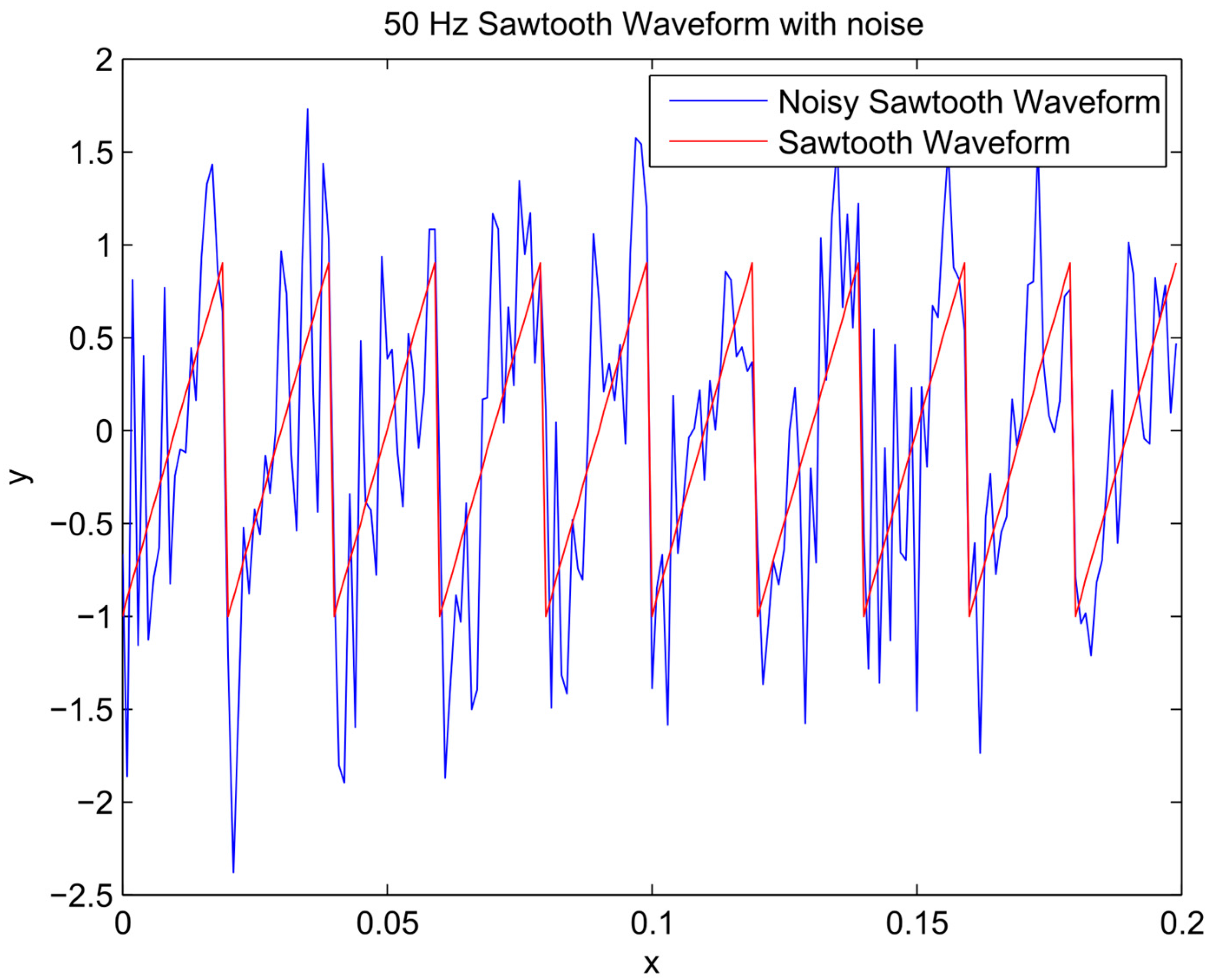
Figure 3.
Composite signal and noisy signal.

Figure 4.
Variation of ensemble models’ entropy (sinusoidal signal).

Figure 5.
Variation of ensemble models’ entropy (sawtooth wave).

Figure 6.
Variation of ensemble models’ entropy (composite signal).
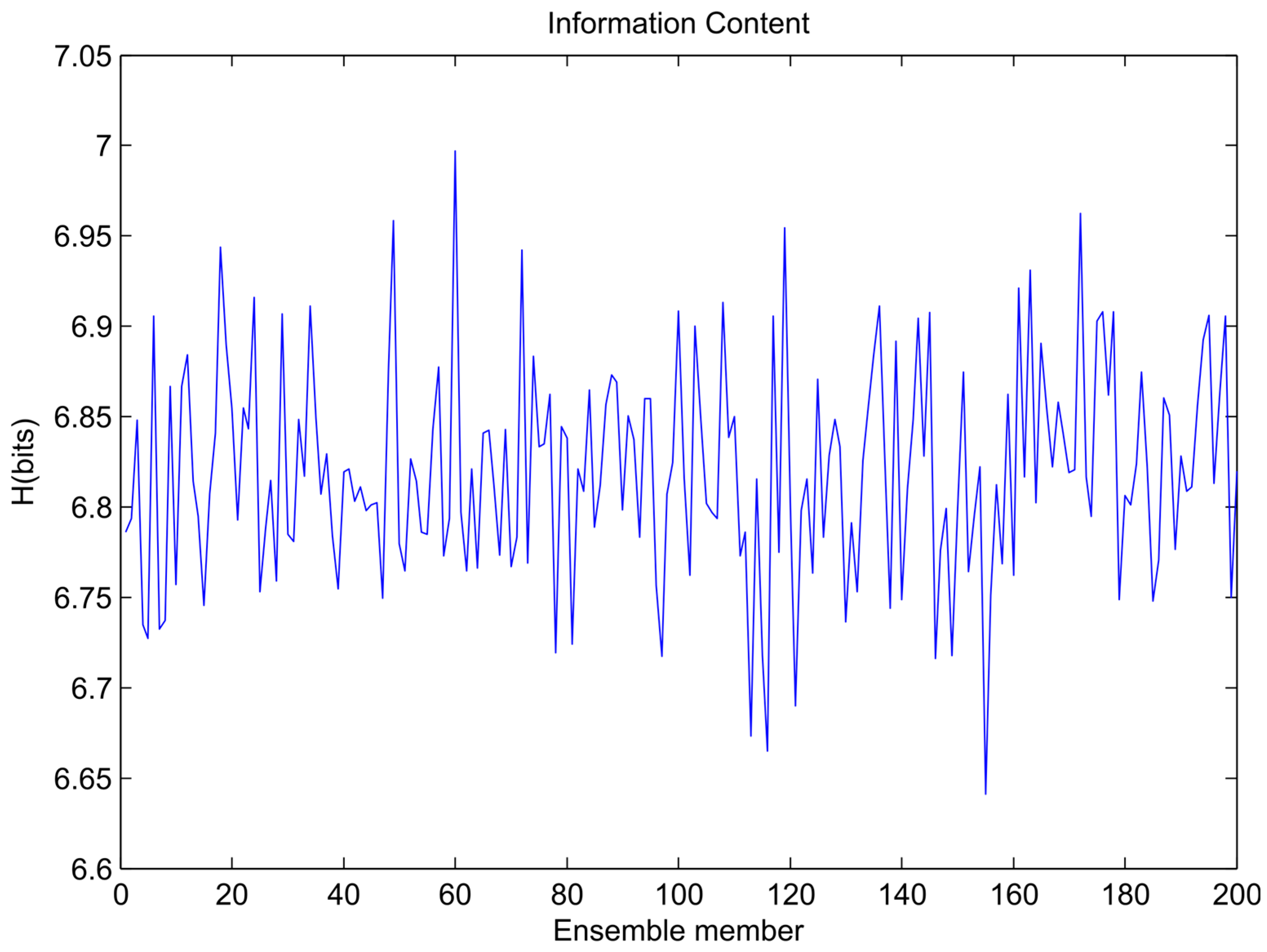
Figure 7.
Sinusoidal signal simulation results.
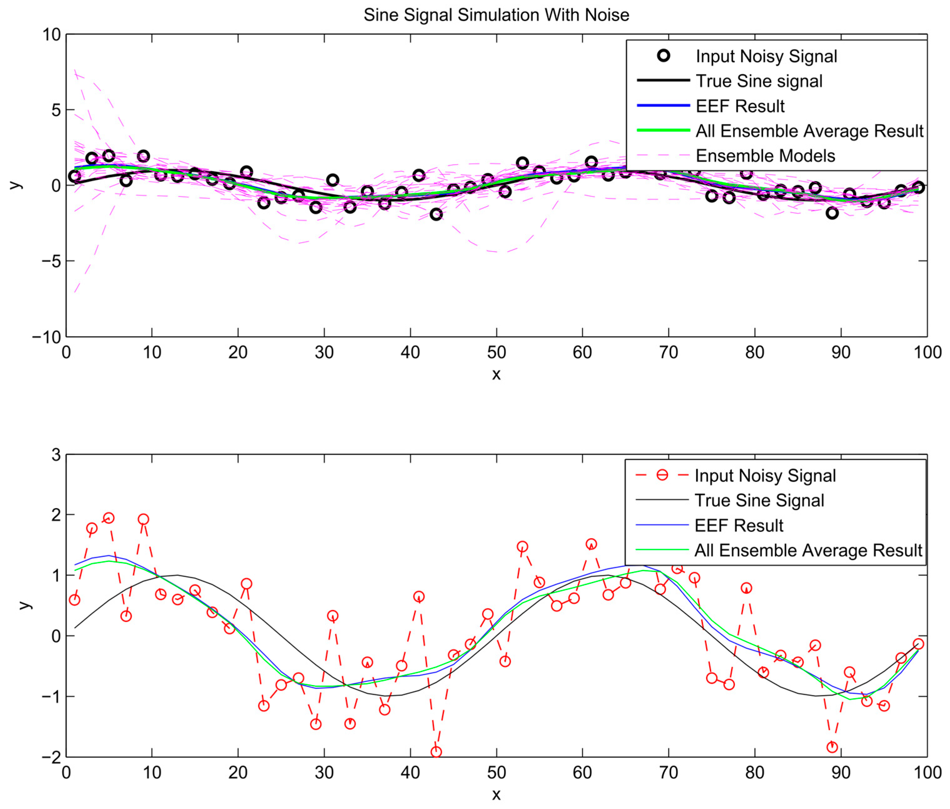
Figure 8.
Sawtooth signal simulation results.
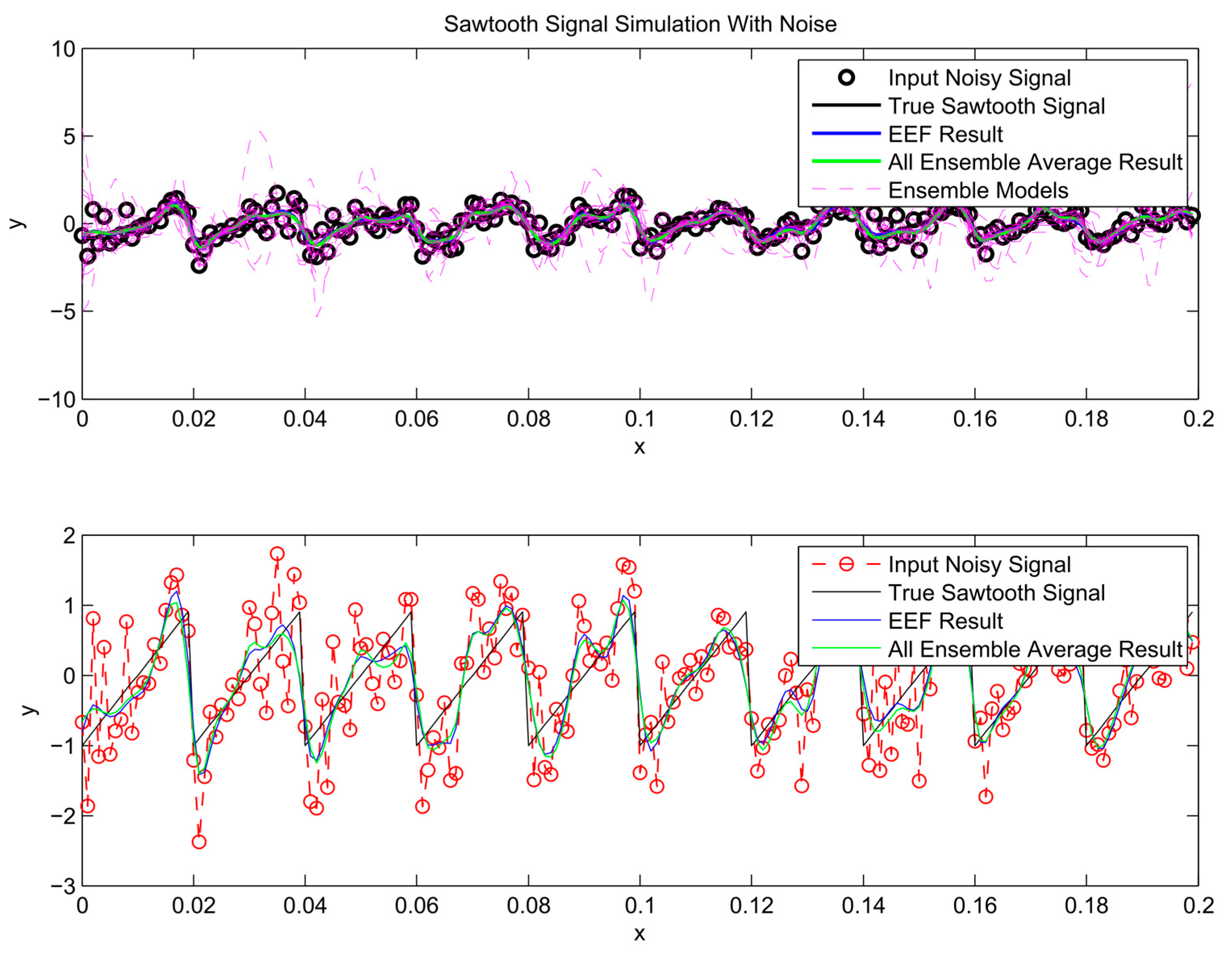
Figure 9.
Composite signal simulation results.

Figure 10.
The error gradient analysis for sinusoidal signal and 100 initial bootstrapped ensembles.
Figure 10.
The error gradient analysis for sinusoidal signal and 100 initial bootstrapped ensembles.

Figure 11.
The error gradient analysis for sawtooth signal and 100 initial bootstrapped ensembles.
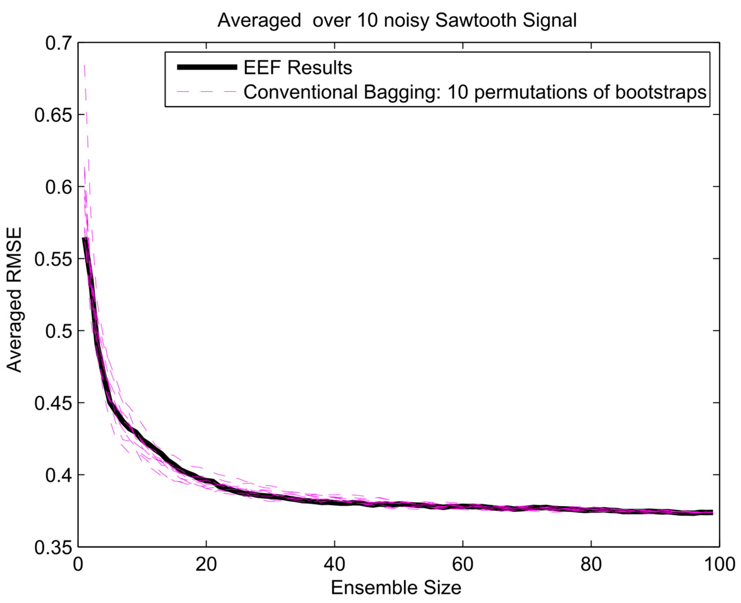
Figure 12.
The error gradient analysis for composite signal and 100 initial bootstrapped ensembles.
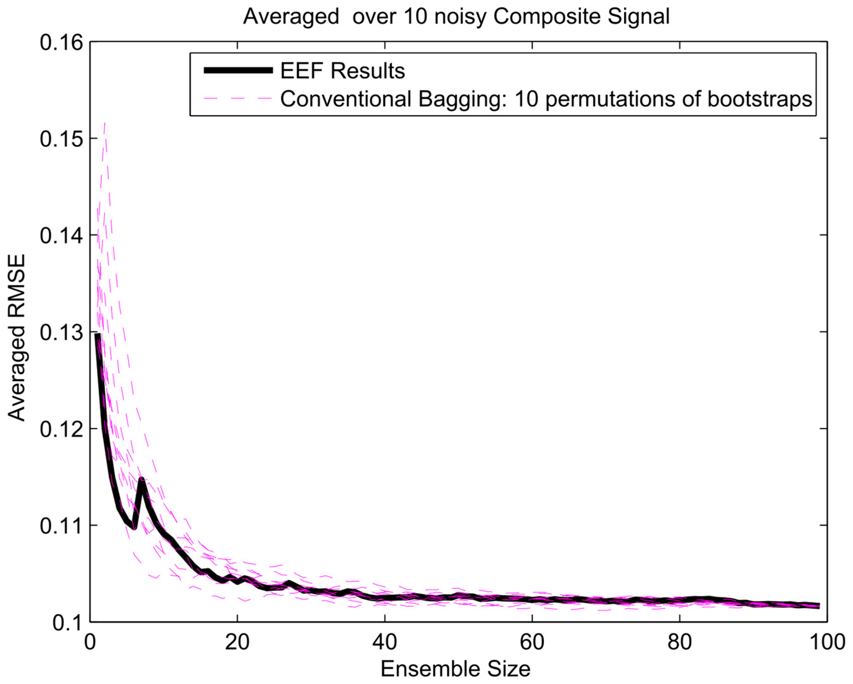
Figure 13.
The error gradient analysis for sinusoidal signal and 1000 initial bootstrapped ensembles.
Figure 13.
The error gradient analysis for sinusoidal signal and 1000 initial bootstrapped ensembles.
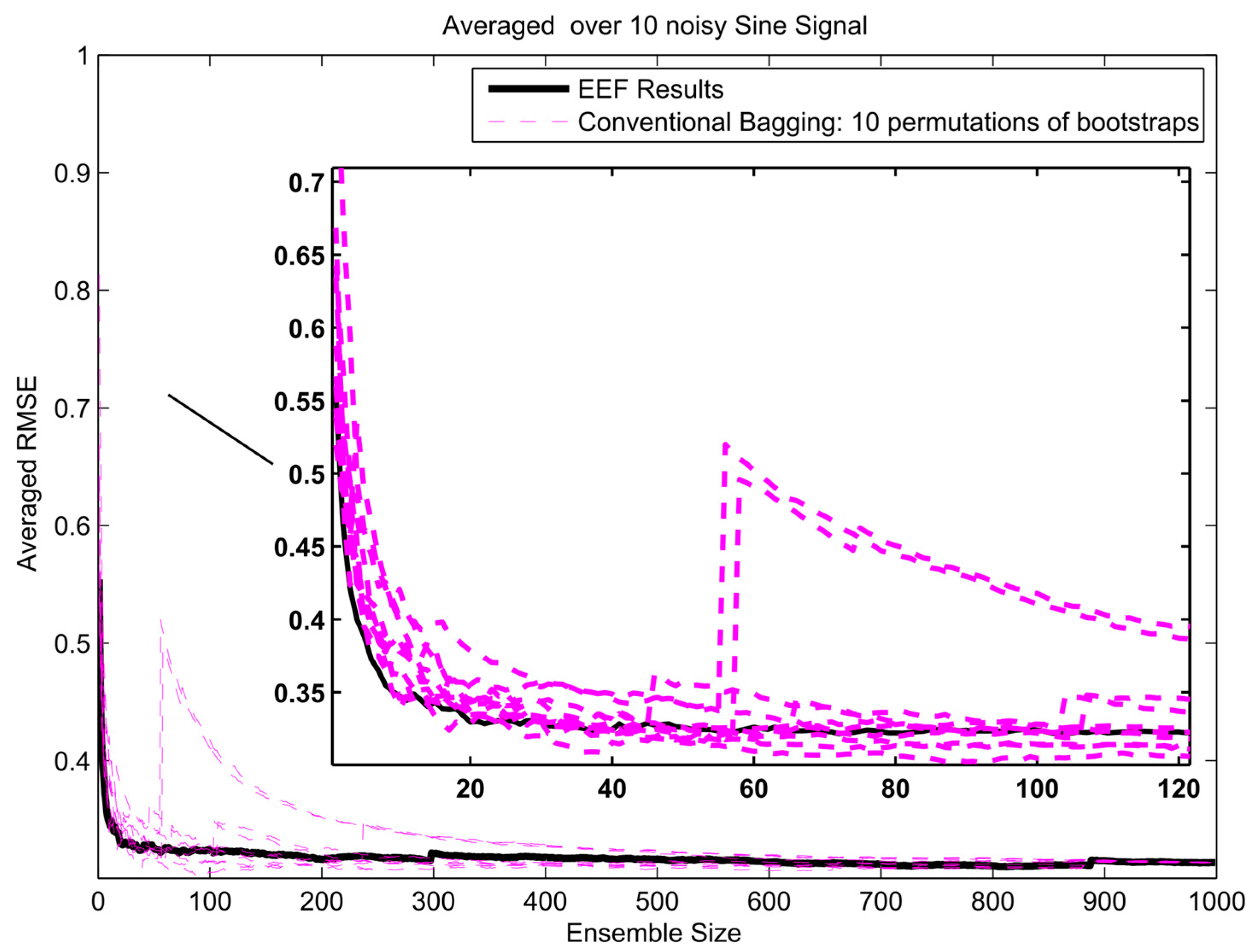
Figure 14.
The error gradient analysis for sawtooth signal and 1000 initial bootstrapped ensembles.

Figure 15.
The error gradient analysis for composite signal and 1000 initial bootstrapped ensembles.
Figure 15.
The error gradient analysis for composite signal and 1000 initial bootstrapped ensembles.

© 2017 by the authors. Licensee MDPI, Basel, Switzerland. This article is an open access article distributed under the terms and conditions of the Creative Commons Attribution (CC BY) license (http://creativecommons.org/licenses/by/4.0/).
Share and Cite
MDPI and ACS Style
Foroozand, H.; Weijs, S.V. Entropy Ensemble Filter: A Modified Bootstrap Aggregating (Bagging) Procedure to Improve Efficiency in Ensemble Model Simulation. Entropy 2017, 19, 520. https://doi.org/10.3390/e19100520
AMA Style
Foroozand H, Weijs SV. Entropy Ensemble Filter: A Modified Bootstrap Aggregating (Bagging) Procedure to Improve Efficiency in Ensemble Model Simulation. Entropy. 2017; 19(10):520. https://doi.org/10.3390/e19100520
Chicago/Turabian StyleForoozand, Hossein, and Steven V. Weijs. 2017. "Entropy Ensemble Filter: A Modified Bootstrap Aggregating (Bagging) Procedure to Improve Efficiency in Ensemble Model Simulation" Entropy 19, no. 10: 520. https://doi.org/10.3390/e19100520
Note that from the first issue of 2016, this journal uses article numbers instead of page numbers. See further details here.