Cross Entropy Method Based Hybridization of Dynamic Group Optimization Algorithm


1
Department of Computer and Information Science, University of Macau, Macau, China
2
Department of Information Technology, Techno India College of Technology, Kalkata 700156, India
3
School of Computer Science & Engineering, University of New South Wales, Sydney 00098G, Australia
4
School of Computer Science, Lakehead University, Thunder Bay, ON P7B 5E1, Canada
*
Author to whom correspondence should be addressed.
Entropy 2017, 19(10), 533; https://doi.org/10.3390/e19100533
Submission received: 7 August 2017
/
Revised: 21 September 2017
/
Accepted: 29 September 2017
/
Published: 9 October 2017
(This article belongs to the Special Issue Entropy-based Data Mining)
Abstract
:Recently, a new algorithm named dynamic group optimization (DGO) has been proposed, which lends itself strongly to exploration and exploitation. Although DGO has demonstrated its efficacy in comparison to other classical optimization algorithms, DGO has two computational drawbacks. The first one is related to the two mutation operators of DGO, where they may decrease the diversity of the population, limiting the search ability. The second one is the homogeneity of the updated population information which is selected only from the companions in the same group. It may result in premature convergence and deteriorate the mutation operators. In order to deal with these two problems in this paper, a new hybridized algorithm is proposed, which combines the dynamic group optimization algorithm with the cross entropy method. The cross entropy method takes advantage of sampling the problem space by generating candidate solutions using the distribution, then it updates the distribution based on the better candidate solution discovered. The cross entropy operator does not only enlarge the promising search area, but it also guarantees that the new solution is taken from all the surrounding useful information into consideration. The proposed algorithm is tested on 23 up-to-date benchmark functions; the experimental results verify that the proposed algorithm over the other contemporary population-based swarming algorithms is more effective and efficient.
1. Introduction
The increasing complexity in modern engineering designs and systems, demands for advances in search algorithms for optimization and analysis [1]. Using traditional methods to solve complicated optimization problems may be inefficient. In light of this, many researchers look into nature which is always a rich source of inspiration. Many well-known meta-heuristic algorithms have been proposed to solve combinatorial problems. For example, the genetic algorithm (GA) [2], particle swarm optimization (PSO) [3], wolf search algorithm (WSA) [4] and dynamic group optimization algorithm (DGO) [5,6,7]. Despites the success in global optimization problems, meta-heuristics algorithms still suffer from several drawbacks. The two most prominent drawbacks are premature convergence and lacking of diversity in evolved solutions. GA and PSO have disadvantages in the exploitation of unexplored search space, and the search agents get easily stuck into a local optimum. The local optimum would be mistaken as the final optimal result where there may often be better optimal points elsewhere. As a result the search ended earlier than it should be, which is called premature convergence. On the other hand, although contemporary algorithm like DGO shows good ability of exploration, it still suffers from the singularity of population. In each round of evolution, the updating information always comes from the same group.
The dynamic group optimization algorithm (DGO) is one of the latest meta-heuristics algorithms, proposed by Tang and Fong in 2016 [6]. The design is inspired by the intra-society and inter-society communications and the interactions of animals including humans. In a DGO system, the population is divided into several groups. Each group has a head and several members. The head corresponds to the best solution obtained so far by the group. The members search around the head to locate the optima by cooperation within the group and by communication amongst groups, the DGO algorithm is half evolutionary algorithm (EA) and half swarm intelligence based algorithm (SI). In the intergroup communication action, the heads can be considered as particles like PSO that move through the search space; this action is a typical SI. However, in the intragroup cooperation action, members evolve based on the information of the heads and the global best solution obtained so far, so it belongs to EA. Since the evolution of population was mainly based on group’s information, the population lacks of varieties and hampers evolution.
DGO is compared to the other metaheuristic algorithms, such as GA, PSO, and DE, it shows numerous advantages. The most distinctive improvement by DGO over the other algorithms is that the other algorithms are influenced by either a global optimum or its own best solution previously obtained so far. They lack of cooperation amongst groups, and different groups never share information. For example, for PSO and most of the population based algorithms, they update solutions just based on the global information and the best solution found from the previous generations. For GA, DE, and their variants algorithms, they produce new solutions according to parent information. On the other hand, DGO has a cooperation mechanism, heads are the delegates of the groups, they not only provide the direction of movement for group members, but also provide for communication channels amongst groups. Moreover, various movement patterns are used in DGO algorithm, the heads use flight to expand the scope of exploration. And it uses two classical mutation operators to exploit the local area and accelerate the convergence. All those advantages shows that DGO is a promising optimization tool. However, the two mutation operators in intragroup action tend to limit the diversity of the population. In addition, the DGO algorithm has a selection mechanism that can maintain the quality of the solution where a new solution must be better than or on par with the existing one. But if the solution traps in local optima, it cannot jump out. Therefore, how to enhance the capability of local exploitation of DGO is worthy to studying.
Technically, a meta-heuristic algorithm has three recurring steps during the search process. The exploration phase occurs when the algorithm discovers a promising search area, the exploitation phase refers to searching for the most promising solution obtained from the exploration phase as quickly as possible, and the escape mechanism that helps the solution avoid the local optima. Many methods are applied in these three steps to improve an algorithm’s performance, such as chaotic mapping, fussing algorithms, and hybrid methods. Many studies have used the above methods to achieve efficient performance [8,9,10,11]. For instance, the cross entropy method (CE) [12] that was proposed by Rubinstein in 1997 was first adopted in the design of an optimization algorithm. In [12], CE was used to enhance an adaptive variance minimization algorithm for solving combinatorial optimization problems. Simply put, the CE method involves an iterative procedure where it has two phases: firstly, a random data sample is generated according to some specified rules. Secondly, it updates the parameters based on the data and reproduces “better” samples in the next generation. The CE method deals successfully with both deterministic problems, such as traveling salesman problem and noisy problems such as buffer allocation problem.
One of the approaches to improve the search ability of optimization is the association of two or more algorithms in order to obtain a better solution or to counteract their drawbacks. Choosing a suitable combination of algorithms for hybridization can be an essential part of achieving better performance in many optimization problems. In this research work, the motivations for combining CE and DGO are as follow:
- The proposed algorithm aims at using CE to enhance the population diversity at local exploitation in DGO.
- It is interesting to set a new local optima avoiding mechanism to help DGO to strengthen the escape ability from premature convergence.
- To the best of our knowledge, the hybridization between these two methods has not been done before. It is an interesting approach to hybridize both methods in order to achieve better optimization performance.
Therefore, to improve the efficiency for finding the best solution and avoiding the local optima, a new hybrid meta-heuristic algorithm called the cross entropy dynamic group optimization (CEDGO) algorithm is proposed in this paper. We use a CE method to update the members and set a time-to-live (TtL) variable to overcome the local optima problem. For comparison with the classical DGO algorithm, 23 benchmark functions are used to test the performance of the CEDGO algorithm.
This article is structured as follows. In Section 2, a brief explanation of CE and DGO is given. Information about types of hybridized methods, and the proposed new algorithm CEDGO is described in Section 3. The results of the experimentation and an analysis of the results are presented in Section 4. Finally, a conclusion and further research are presented in Section 5.
2. Background
2.1. Cross Entropy Method
The cross entropy method for optimization can be described as follows.
where is the maximum over the given set X, the is the maximal x. S is the performance metric. When estimating samples X iteratively, a set of indicator functions are defined. represents the S(x) as above in the level for sample x. For a vector u, m of probability density function parameters, the optimization problem can be transformed into estimating the probability . Combining with indicator functions, the probability can be calculated by:
where P is the probability associated with the probability density function f(., u), and denotes the expectation function. If , can be estimated as:
is generated by using the pdf f(., v). It is worthy to note that the CE method finds the most well sampling density f(., v*) such that the optimal solution can be sampled [13].
The procedure of CE can be summarized into three main phases:
- Generate random samples from Gaussian distribution with mean mu and standard deviation s.
- Select a specific number of best samples from the whole samples.
- Update mu and s based on the best samples with better fitness.
The Algorithm 1 of CE for optimization is listed as follows:
| Algorithm 1: pseudo code of CE method |
| Initialize: mean mu, standard deviation s, size of population pop, the number of best samples np, terminal condition tmax |
| While t < tmax do |
| Generate sample vectors X as: |
| , where randn() produces a Gaussian distribution random number. |
| Evaluate xi |
| Select the np best samples from pop |
| Update the parameters mu, s |
| t = t + 1 |
| End |
2.2. Dynamic Group Optimization Algorithm (DGO)
Dynamic group optimization is the latest optimization algorithm, which is inspired from the intra-society and inter-society communication and the interactions of animals. Three main actions are summarized, first, intragroup cooperation, second, intergroup communication and third, group variation. All possible solutions, divided into two parts: members and heads, they are randomly initialized. For the intergroup cooperation, members are updated by Equations (4) and (5), respectively,
where the is the vector of kth dimension of jth member of the ith group, which is obtained randomly from the whole populations. is the kth dimension value of the ith head. G is the generation. b is the best solution obtained so far. The is an index of group head, which is chosen randomly and the is the random number generator, the produced value is between [0, 1]. is drawn from normal distribution with mean 0 and standard deviation 1. r1 and r2 are indexes of two distinct individuals, which are chosen randomly (exclude heads). Mr1 and Mr2 are two values between [0, 1], which are set by user to control the mutation probabilities of the two parts.
In order to enhance the ability of global exploration, the intergroup communication utilizes flight walk as the walking pattern. Heads as the group’s delegate communicate with the other groups in this phase. There is only head that can update. The movement uses the levy flight random walk. The mathematical update equation of levy flight walk is formulated by Yang [14] as follow:
The is the entry-wise multiplications. and mean the ith group in the k + 1 and k generations. is a random number, which is drawn from distribution. The is a scaling factor, the is the global best solution. Equations (6) and (7) are the formula of head updating. Heads move towards global best by using Lévy flight walk. The exponential form of probability function is:
The last action is group variation, this action avoids the waste of computing. Put simply, the better fitness, and the more members are in the group.
From Equations (4) and (5), we can find that the intragroup action of DGO is composed of two mutation operators. However, the operators cannot make great contribution to the population diversity, resulting in limiting the search ability of DGO. Moreover, the search ability of DGO may be deteriorated if the two randomly selected solutions for mutation is not significant enough.
In order to investigate the contribution of gaining diversity by using mutation, we carry out an experiment. We use the diversity measure to show the population diversity. The mathematical formula shows as follows:
where N is the size of population set, |N| is the size of set, |L| is the length of longest diagonal in search space, D is the size of dimension, is the jth value of the ith individual, and is the average value of the jth dimension value of all the agents in the population. We compare the diversity between DGO without mutations and normal DGO (inDGO) at different dimensions where D = 10, 30, and 50. The test function is sphere. The diversity is shown in Table 1.
From Table 1, in DGO has better diversity than DGO on all dimensions. Hence, it indicates that the mutations merge the whole population together hence deteriorate the search ability. How to solve this problem is the main focus in this paper.
3. Cross Entropy Dynamic Group Optimization (CEDGO)
In order to overcome the limitation of the original DGO, a cross entropy method based dynamic group optimization algorithm (CEDGO) is proposed. In this section, the detail of the proposed algorithm is presented.
In our proposed algorithm, the CE is used to cover the lack of exploitation of intragroup action, focusing the search of solutions in the area where the best solution located. Therefore, the intragroup action of DGO is replaced by CE. The DGO is mainly responsible for the exploration, and the CE is modified to a CE operator, which is employed into the intragroup action. The CEDGO takes advantage of the exploration ability of DGO and the exploitation ability of CE. Moreover, we set a time-to-live mechanism to control the density of population distribution.
The CEDGO works in this way: first, it initializes all parameters and generates population randomly. Then, it divides the population into a specific number of groups and selects a head for each group. At each iteration/generation of the algorithm, the heads move by the levy flight patterns while the members update themselves by the CE operator. Once every agent in the population is updated, the time to live (TtL) of each one is calculated. If the value of Ttl is lower than a threshold, the corresponding solution is reproduced randomly to avoid being stuck into a local optimum. The Algorithm 2 of CEDGO describes as follows.
| Algorithm 2: pseudo code of CEDGO method |
| Initialize: group numbers np, mean mu, standard deviation s, size of population pop, the number of best samples np, terminal condition tmax |
| Select group heads according to the fitness |
| While t < tmax do |
| Head moves by using levy flight (6). |
| Members moves by using CE operator (3). |
| Update the mu and s according the fitness. |
| Calculate the TtL |
| Group variation |
| Evaluate all population |
| Select new group heads |
| t = t + 1 |
| End |
3.1. Cross Entorpy Operator
The cross entropy operator is used for updating the members’ position. The mean mu and standard deviation s are the most important parameters in this operator. The mu tends to locate itself over the point with the best results, while s becomes smaller, until both values are focused on the area of the best solutions found so far in the domain. The variation of these values is done with a parameter indicating the learning rate (Lr).
The new samples are generated by mu and s. The mathematical equation is defined as follows:
where randn() produces the Gaussian distributed random number.
The parameters update is done using (11) and (12).
where Mu = (mu1, mu2, …, mun) and the standard deviation S = (S1, S2, …, Sn). For each i in a vector, a random number is generated by a Gaussian distribution N(mu1, s1).
3.2. Time-to-Live Mechnism (TtL)
The classical DGO uses simple greedy strategy to keep good solutions and discard worse solution. The main deficit is that it lacks of an escape mechanism, solution may falls into local optima and unable to extricate itself. The time-to-live mechanism design makes individuals born and die dynamically, thus they inherit good information from ancestors as well as being able to escape from local optima. The basic principle of TtL is similar to natural selection, where only the fittest will survive. All individuals are considered as natural creatures, it is universal knowledge that all living creatures go through life-cycle of birth, aging, illness, and death. Analogically speaking, if an animal is given plenty of foods (metaphor of computing resource in running meta-heuristics), it will have a longer life span than the one that has little food.
The “TtL” represents that the individual only can live within a variable length of time which depends on whether the food is adequate or not. If an individual cannot find enough food within the length of time, it will die. On the contrary, enough food is expected to prolong survival still further. Since the total population is stable, therefore, when one individual dies, another new individual will be born.
The TtL mechanism is defined by the following rules:
Numbered lists can be added as follows:
- Rule (a)
- Each individual will only be graced a certain length of times to live when the animal shows inability to obtain any better food.
- Rule (b)
- The individual will die when the animal still yields no better food after the length of times to live are used up.
- Rule (c)
- The individual’s health condition stays the same as long as it finds better food.
- Rule (d)
- New individual is produced by obtaining three randomly selected heads’ information.
The rule (a) enforces a contesting environment, where only competitive individuals can live longer. The rule (b) reduces the chances of an individual who is wasting computer resource. The rule (c) keeps the better individuals alive so to continue producing better result. The rule (d) is a way to generate new solution and it keeps good information from ancestors.
The solutions will have differential lifetimes depending on how competitive they are in continuously finding improved candidate solution over the search space. This mechanism guarantees the search agent will not be doing useless work consuming computing resources unnecessarily when it is into local optimum.
To investigate the diversity of population of CEDGO. The results represents in Table 2:
From Table 2, cross entropy dynamic group optimization (CEDGO) outperforms the DGO and DGO without mutations and normal DGO (inDGO) in terms of diversity at the three dimensions.
3.3. Complexity Analysis
Assume D is the dimensionality of the search space, the MaxFEs is the maximum number of function evaluation number, and the Cof is the cost of the objective function. Basically, an evolutionary algorithm has a time complexity of O(N × MaxFEs + Cof × MaxFEs). However, the time complexity of most objective functions is O(n) or even higher and different objective functions have different time complexities depending on how the fitness is computed or derived. For instance, the Rastrigin function has complexity O(n). But the complexity of rotate Rastrigin function scales up to O(n2). Therefore, usually the Cof contributes more substantially to the time complexity. The whole time complexity is determined by the objective function.
In order to analyze the complexity of our new algorithm, despite the Cof, we first calculate the time complexities of DGO and CEDGO. The costs of the classical DGO algorithm involve the initialization (Tini), evaluation (Teva), three actions (Tinter, Tintra, Tvari) and selection Tsel Here, Tinter = D, Tintra consists of two mutation operators. So that Tintra = 2D, Tvari = 1, Tsel = D. Therefore, the time complexity of traditional DGO can be estimated as T(D) =Tini + (Teva + Tinter + Tintra + Tvari + Tsel) × MaxFEs = D + (D + D + 2D + 1 + D) × MaxFEs = D + (5D + 1) × MaxFEs. So, O(D × MaxFEs) is the time complexity of DGO.
CEDGO involves three identical components as DGO, but Tintra is changed. Tintra is replaced by CE operator, Tce is equal to D. The TtL is added in CEDGO, the Tttl = D as well. Therefore, T(D) = Tini + (Teva + Tinter + Tce + Tvari + Tsel + Tttl) × MaxFEs = D + (D + D + D + 1 + D + D) × MaxFEs = D + (5D + 1) × MaxFEs. It is the same time complexity of DGO, which linear to MaxFEs.
4. Experimental Results
To fully evaluate the performance of the CEDGO algorithm without a biased conclusion, we conduct different experiments. Twenty-three benchmark functions are used in our experimental studies. These functions have been widely used in numerous studies [15,16]. In this test suite, F1–F7 are unimodal functions, F8–F13 are multimodal functions with a high dimensional scale and F14–F23 are multimodal functions with a limited dimension scale. They appear to be the most difficult class of problems for many optimization algorithms. The results are very important because they reflect an algorithm’s ability to escape from poor local optima and locate a good near-global optimum. The dimension of this function is chosen at 30. In addition, we investigate whether the CEDGO algorithm could be scaled up to handle large-scale optimization problems. Therefore, for the high dimensional functions F1–F13, the dimensions scale up to 300, larger than those in many other studies. This is necessary because as the number of dimensions increases, their local optima increase exponentially. In real life optimization problems, most cases are high dimensional problems; and if the scale is small, it would be very difficult to make generalized conclusions over the comparison. The focus of the study is to compare the performance of the CEDGO algorithm with the classical DGO algorithm; however, to investigate the CEDGO algorithm comprehensively, we also compare the performance of the CEDGO algorithm with that of other famous EAs algorithms. Moreover, an efficiency comparison with a parameter tuning is carried out.
In addition, to show the performance of the DGO algorithm, we compared it to four well-known improved DE algorithms, including DE with strategy adaption (SaDE) [17], self-adaptive DE (jDE) [18], composite DE (CoDE) (24), and adaptive composite DE (ACoDE) algorithms [19].
Two types of performance criteria are used in our experiment. First, the average and standard deviation of the function value are used. The algorithms run 50 times on each benchmark function, and the average and the standard deviation of the value are calculated. The notation AVGr ± SDr is used in Table 4. Second, the Wilcoxon rank sum test is used to test the significance between the algorithms. The p value, as an informal measure of evidence against the null hypothesis, is listed in different Tables. The “-” symbol shows that the null hypothesis is rejected when the p value is equal to or less than the significant level and the first algorithm outperforms the second one. The “+” symbol means that the null hypothesis is rejected when the p value is equal to or less than the significant level and the first algorithm is inferior to the second one. The “=” symbol reveals that the null hypothesis is accepted when the p value is greater than the significant level and the first algorithm is equal to the second one. The test at a significance level where α = 0.05 is applied.
In order to obtain unbiased results, all experiments were carried out at the same experimental condition, for each algorithm, the maximum number of fitness evaluations (FEs) is 10,000 × D, D is the dimension of the problem, we set it as 30, except the high-dimensional problem where D = 300. Each algorithm is run 50 times independently to obtain average and the other statistical results. The experiments are run in Matlab R2015a (The MathWorks, Natick, MA, USA), CPU is Intel(R) Core i7-4790 @ 3.60 GHz (Intel, Santa Clara, CA, USA) RAM is 8.00 GB. The global optimization toolbox used in our experiment includes GA and PSO algorithms. The GA used heuristic crossover, the roulette selection function and feasible adaptation mutation. The mutation rate and crossover rate were set to the default values. We also used the standard PSO algorithm; c1 and c2 used a default value of 1.49. In the WSA, the visual distance is 0.3 and the pa is 0.25. BA used the default setting from the public Matlab code, which was obtained from the MathWorks community. For DE algorithms, the parameter settings adopt a scaling factor F = 0.9 and crossover rate Cr = 0.9 for all algorithms. For the parameter settings of the DGO algorithm, we set the mutation rate and crossover rate to 0.25. The size of population is crucial in algorithms, so we used the same population size (30) for all algorithms. For PSO variant algorithms, the c1 and c2 are equal to 2, which are suggested by [20]. The maximum weight is 0.9 and the minimal weight is 0.4 for all PSO variant algorithms. And for the DE variant algorithms, LP = 50 in SaDE, the τ1 = τ2 = 0.1 in jDE, F = 0.9 in ACoDE and CoDE. It is worthy to mention that the parameters for some algorithms are adjusted automatically, for example, the c1 and c2 of IPSO changed dynamically. Therefore, the values of the parameter settings remain the same since they were set initially.
In our experiments, all parameters are the same, and the population size is 30 with the same set of initial random conditions. We also use the PSOs, and the c1 and c2 assume the default value of 1.49. The experimental environment is shown in Table 3.
4.1. Effect of CEDGO
Table 4 lists the means and SDs of the function values obtained from comparison between DGO and CEDGO.
4.1.1. Unimodal Functions
Table 4 lists the average and standard deviation of the function values in 50 runs. The results generated from the DGO algorithm are tabulated in Table 4 and compared with the results generated by our CEDGO algorithm. The results show that our proposed CEDGO algorithm outperforms the DGO algorithm on all unimodal functions except F7. For functions F1, F2, and F6, the CEDGO algorithm generated significantly better results than the classical DGO algorithm. Although the DGO algorithm outperforms the CEDGO algorithm on function F7, the result is insignificant. The p value is also reported in Table 4; it can be seen that the CEDGO algorithm outperforms the DGO algorithm in five functions, ties with the DGO algorithm in one function and loses to the DGO algorithm in one function. In summary, the search performance of the CEDGO algorithm is generally better than that of the DGO algorithm on unimodal functions.
4.1.2. Multimodal Functions
Functions F8–F23 are multimodal functions. Table 4 clearly shows that the CEDGO algorithm wins in most of the functions. The CEGDO algorithm outperforms the DGO algorithm on eight of the 16 functions, ties with the DGO algorithm on four functions and loses to the DGO algorithm on four functions. Functions F7–F13 are multimodal functions with many local minima, which are very difficult to optimize. Generally, the CEDGO algorithm outperforms the DGO algorithm on two of six functions. But for function F11, the CEDGO algorithm performs significantly better than the DGO algorithm. From the p value, the CEDGO algorithm shows better performance than the DGO algorithm on two of the six functions, ties with the DGO algorithm on two functions and loses to the DGO algorithm on two functions. It shows that the CEDGO algorithm has the same performance on multimodal functions with many local minima. Functions 14–23 are multimodal functions with few local minima. With this set of functions, it is relatively easy to find the optima due to the dimension scale. From Table 4, we can see that the CEDGO algorithm outperforms the DGO algorithm on six of the 10 functions and ties with the DGO algorithm on four functions; it loses none. The p value shows a similar result: the CEDGO algorithm shows better performance than the DGO algorithm. From these 23 benchmark functions, we can summarize that the CEDGO algorithm exhibits better performance and greater robustness than the classical DGO algorithm on these benchmark functions, due to the effect of the CE operator.
Figure 1 shows the convergence diagrams, with 500 iterations and the dimension D = 30. The other experimental setting is the same as that described in Section 4. Figure 1a,b are results of unimodal functions, we can easily observe that the CEDGO is faster than the DGO on convergence. Particularly, on function F3, DGO seems stuck into local optima very early, and CEDGO can continue the search. The multimodal functions can also draw the same conclusion from benchmark functions F10 and F14. From Figure 1, it is can be seen that CEDGO has more zigzags in the convergence curve. It is because the CEDGO has more chances to use CE operator and TtL mechanism to increase the diversity of population; hence there are more chances to jump out from local optima.
4.2. Comparison with the Latest Variant PSO Algorithms
The PSO algorithm is a population-based swarm intelligence optimization algorithm that was first introduced in 1996 by Kennedy et al. It is efficient in solving optimization problems. To fully investigate the performance of the CEDGO algorithm, we compare the CEDGO algorithm and the latest variant PSO algorithms, including autonomous particles group particle swarm optimization (AGPSO) [20], improved particle swarm optimization (IPSO) [21], time varying acceleration particle swarm optimization (TACPSO) [22] and modified particle swarm optimization (MPSO) [23]. Table 5 lists the results of the comparison.
From Table 5, it can be seen that the CEDGO algorithm obtains the highest accuracy on the most functions. The CEDGO algorithm outperforms the PSO algorithms on six of the seven unimodal functions, three of the six multimodal functions and six of the 10 multimodal functions with few minima. The CEDGO algorithm has significantly better performance than the PSO algorithms. Table 5 reveals that the CEDGO algorithm is the best and is superior to the PSO algorithms.
4.3. Comparison with the Other Well-Known Evolutionary Algrotihms (EAs)
This section reports the comparison between the CEDGO algorithm and four well-known EAs: the bat algorithm (BA) [24], the PSO [3], the GA [2], and the WSA [4]. Many studies have shown that those algorithms are good at solving global optimization problems. The CEDGO algorithm was tested with the same benchmark function at D = 30 with 50 independent runs. The average function values and standard deviations are recorded. The parameter setting shows at Table 6.
It can be seen from Table 7 that the CEDGO algorithm is significantly better than the other algorithms on most functions. In terms of the accuracy of the average function values, the CEDGO algorithm is good at all functions except F7, F9 and F15. The CEDGO algorithm obtained the best result 20 times and the second-best result three times for the 23 functions we tested; the CEDGO algorithm converge near the optimal solution. The results prove that CEDGO algorithm can achieve satisfactory results on those testing functions when compared with these EAs.
4.4. Scalability Study
In the real world, many optimization problems have hundreds of variables or even more. So far, we have shown that our proposed CEDGO algorithm generates good results for 30-dimensional problems. To investigate the effects of this problem on the performance of the CEDGO algorithm, we carry out a scalability study with the classical DGO algorithm, the other EAs, and the CEDGO algorithm. Because F14–F23 are low-dimensional benchmark functions, the set of benchmark functions F1–F13 are extended to 300 dimensions. The results are shown in Table 8.
Table 8 shows that, in terms of average function value, the CEDGO algorithm outperforms the other algorithms on F1–F7. The CEDGO algorithm generates the best performance on four of the seven functions on unimodal functions. For F8–F13, the CEDGO algorithm gave the second-best results, obtaining the best performance on one occasion. The CEDGO algorithm is significantly better than the EAs. In summary, the performance of these algorithms on 300 dimensions at unimodal functions F1–F7 falls in the order CEDGO > DGO > BA > GA > WSA > PSO. For functions F8–F13, the order is DGO > CEDGO > BA > GA > WSA > PSO.
4.5. Parameters Tuning Study
To investigate the sensitivity of the CEDGO algorithm to the coefficient α, we carry out an experiment with = 0.25, 0.5, 0.65 and 0.8 respectively. The other parameters used the same values as those presented in the previous sections. The results are reported in Table 9.
Table 9 shows that the performance of the CEDGO algorithm is sensitive to the learning rate ; for unimodal functions, the best performance is obtained by Lr ; it reaches the best optima five times. For multimodal functions with many minima, the Lr = 0.5 is the best, winning three out of six functions. Lr = 0.5 is the best for the multimodal function with few minima.
4.6. Comparision with DE Algrotihms
DE algorithms are amongst the most well-known optimization algorithms; they are population-based stochastic optimization algorithms, exhibiting overall excellent performance for many benchmark functions. Therefore, we compared the DGO algorithm and several improved versions of the DE algorithm with a dimension size of 30 and a population size of 30. Table 10 shows the means and standard deviation of the function values when the number of evaluations is 10,000 × D.
In Table 10, in terms of the average function values, the DGO algorithm shows the same performance as the other algorithms on F14, F16, F17, F19, and F23; all searches can find the global optimum. Compared with the DE algorithms, the DGO algorithm yields the best performance on F3. In addition, the CEDGO algorithm obtains the best result most of the times.
4.7. Algorithm Analysis and Disscusion
In CEDGO, the CE operator is employed, which updates solutions by using the mean and standard deviation of solutions. The mean mu assures that the new solutions are produced based on the whole population’s information, not just focuses on the current group and just uses two mutations in the DGO.
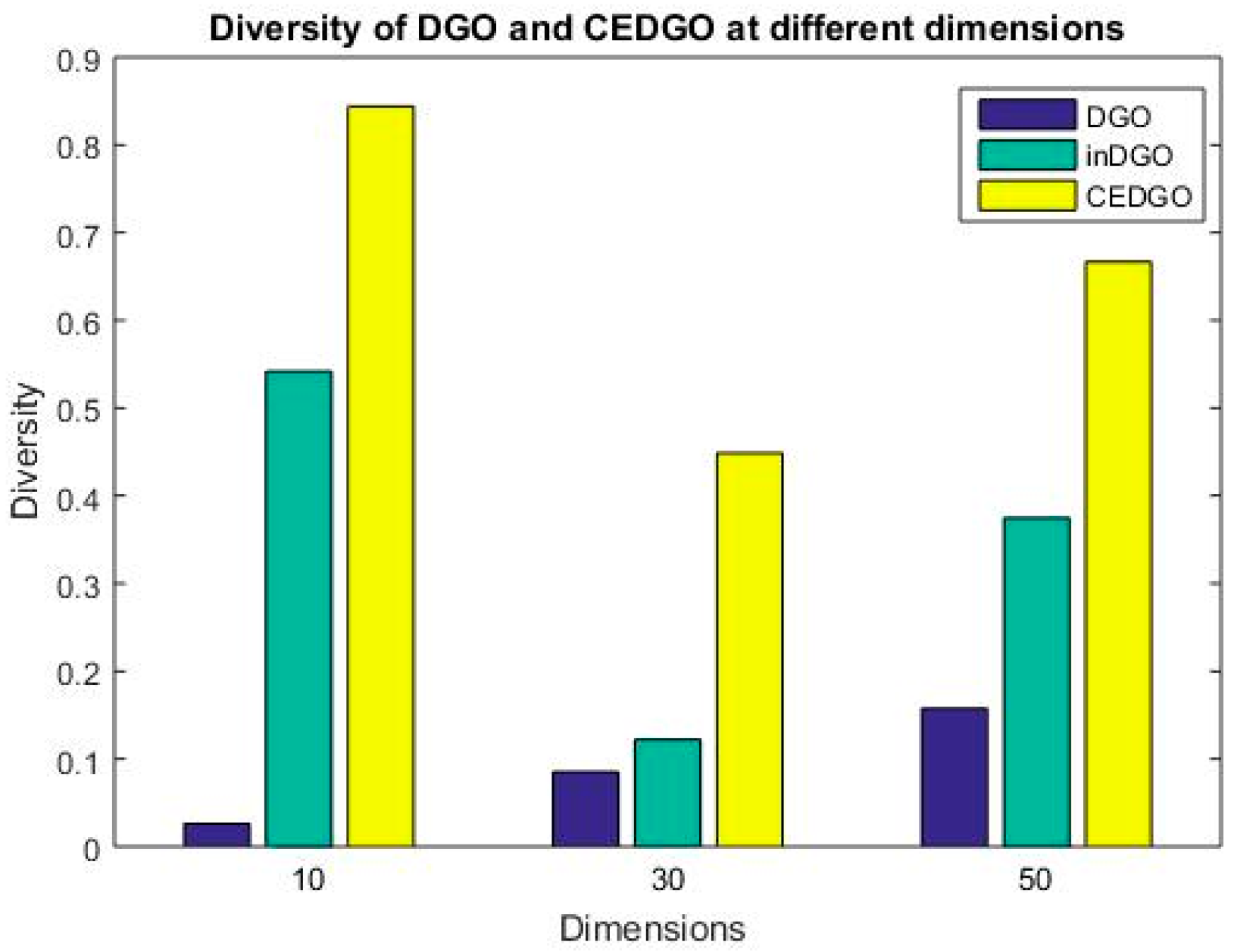
The deviation limits the range of new solutions, which determines the movement tendency. The selected samples in the CE operator are the best individuals from the populations, it ensures the robustness of the population. Information is obtained by small fraction of population which may lead to information loss. Moreover, replacing the mutations by CE operator greatly improved the diversity of population. The illustration of diversity of DGOs at different dimensions are shown in Figure 2:
From Figure 2, we can see that our proposed CEDGO outperforms the DGO and in DGO in terms of diversity at all dimensions. The CE operator not only enlarges the promising search area, but also guarantees that new solution take all the surrounding useful information into consideration.
In TtL mechanism, the solutions will have a differential lifetimes depending on how competitive they are in continuously finding improved candidate solution over the search space. In DGO, the group variation only allows one solution to escape the local optima. But in TtL, each solution has a chance to do so in each iteration. In addition, since the CE operator is in use, it accelerates the convergence. Observing from Figure 1, the CEDGO is faster than DGO on optimizing both unimodal and multimodal functions. From the time complexity analysis in Section 3.3 and the experiments in Section 4, the result shows that under the same computation environment, the results of CEDGO is superior to DGO.
DGO lends itself strongly to exploration and exploitation. However, balancing global exploration and local exploitation is still difficult, better global exploration capability is usually accompanied by worse local exploitation, and vice versa. The intragroup action of DGO consists of two mutation operators, all of them exploit the area of promising best optimum intensively. Since the members’ information only can be obtained by group heads, all members merge together towards corresponding heads. The consequence of this is that the diversity of population diminishes quickly after several iterations.
CE has been successfully applied into various applications, one of the famous application is the optimization problems. Cross entropy method has proven to be successful in the solution of difficult single objective real valued optimization problems [25]. The new solutions are generated by the mean and standard deviation rather than just obtain information from the surrounding area. Therefore, the new solutions would not be too crowd at one position. CE has properties of randomness, it is perfectly matched the stochastic feature of meta-heuristic optimization algorithms. The CE operator not only accelerates the speed of algorithm, it can also enhance the variety of movement pattern.
From experimental results in Section 4 on benchmarks, it demonstrates that CEDGO outperforms the classical DGO, moreover. The comparison between CEDGO with PSO variants and EAs indicates that CEDGO is a promising tool for solving optimization problems.
Through the parameter tuning test, it can be concluded that learning rate equals to 0.5 is the most suitable value for CEDGO. In our work, we use the same experiment environment to obtain the unbiased results. However, our benchmark evaluation may generate different results if we change the population size or termination condition. In spite of these caveats, the benchmark results show that CEDGO is a promising optimization tool.
5. Conclusions
CE is a novel approach that has been widely used in various applications. In this study, we used the CE method combined with the novel algorithm DGO to improve the performance of the original DGO algorithm. We proposed a new meta-heuristic namely CEDGO algorithm that has two main activities: first one is, CEDGO replaces the old intragroup actions by CE operator. It enhances the ability of local search and increases the diversity of populations. The second activity is that the time-to-live mechanism is employed into the algorithm. TtL helps the algorithm avoid getting stuck into local optimum, hence it saves computation resources.
The main contribution of this paper can be summarized as follows:
- Because the CE operator is employed into intragroup action, the capability of local search is enhanced.
- Because the original two mutation operators are removed, the diversity is increased.
- The TtL mechanism is set, the computation resource is saved compared to classical DGO.
- Due to the TtL, the capability of jumping out of local optimum is increased.
To investigate the performance of the CEDGO algorithm, 23 benchmark functions were used for comparison. The experimental results show that our proposed algorithm outperforms the other algorithms in different testing conditions. A parameter setting Lr = 0.8 is suggested for solving multimodal functions with many minima. Lr = 0.5 is suggested for solving unimodal problems, and Lr = 0.5 is suggested for solving multimodal functions with few minima problems.
A limitation of this study is that only 23 benchmark functions were used to verify the algorithm’s performance. We plan to carry out more comprehensive benchmark functions in the future to evaluate the proposed method in greater depth. Although benchmark functions are a simple and useful means to test optimization algorithms, they should also be used in real-world applications. Therefore, we plan to apply the CEDGO algorithm to real-world problems as a future study.
Acknowledgments
The authors are grateful for financial support from the research grant for “Nature-Inspired Computing and Metaheuristics Algorithms for Optimizing Data Mining Performance” from the University of Macau (grant No. MYRG2016-00069-FST).
Author Contributions
Rui Tang and Simon Fong were responsible for the research design, data analysis and paper writing. Nilanjan Dey collected the benchmarks, Raymond Wong were responsible for Table making and reformatting the paper. Sabah Mohammed polished the paper. The manuscript was read and approved to submit by all authors.
Conflicts of Interest
The authors declare no conflict of interest.
References
- Yang, X.-S. Nature-Inspired Optimization Algorithms; Elsevier: Amsterdam, The Netherlands, 2014. [Google Scholar]
- Goldberg, D.E.; Holland, J.H. Genetic algorithms and machine learning. Mach. Learn. 1988, 3, 95–99. [Google Scholar] [CrossRef]
- Kennedy, J. Particle swarm optimization. In Encyclopedia of Machine Learning; Springer: Berlin, Germany, 2011; pp. 760–766. [Google Scholar]
- Tang, R.; Fong, S.; Yang, X.-S.; Deb, S. Wolf search algorithm with ephemeral memory. In Proceedings of the 2012 IEEE Seventh International Conference on Digital Information Management (ICDIM), Macau, China, 22–24 August 2012; pp. 165–172. [Google Scholar]
- Tang, R.; Fong, S.; Deb, S.; Wong, R. Dynamic group search algorithm for solving an engineering problem. Oper. Res. 2017. [Google Scholar] [CrossRef]
- Tang, R.; Simon, F.; Suash, D.; Wong, R. Dynamic Group Search Algorithm. In Proceedings of the International Symposium on Computational and Business Intelligence, Olten, Switzerland, 5–7 September 2016. [Google Scholar] [CrossRef]
- Kwiecień, J.; Pasieka, M. Cockroach Swarm Optimization Algorithm for Travel Planning. Entropy 2017, 19, 213. [Google Scholar] [CrossRef]
- Hu, W.; Liang, H.; Peng, C.; Du, B.; Hu, Q. A hybrid chaos-particle swarm optimization algorithm for the vehicle routing problem with time window. Entropy 2013, 15, 1247–1270. [Google Scholar] [CrossRef]
- Wang, S.; Zhang, Y.; Ji, G.; Yang, J.; Wu, J.; Wei, L. Fruit classification by wavelet-entropy and feedforward neural network trained by fitness-scaled chaotic ABC and biogeography-based optimization. Entropy 2015, 17, 5711–5728. [Google Scholar] [CrossRef]
- Xiao, Y.; Kang, N.; Hong, Y.; Zhang, G. Misalignment Fault Diagnosis of DFWT Based on IEMD Energy Entropy and PSO-SVM. Entropy 2017, 19, 6. [Google Scholar] [CrossRef]
- Song, Q.; Fong, S.; Tang, R. Self-Adaptive Wolf Search Algorithm. In Proceedings of the 2016 IEEE 5th IIAI International Congress on Advanced Applied Informatics (IIAI-AAI), Kumamoto, Japan, 10–14 July 2016; pp. 576–582. [Google Scholar]
- Rubinstein, R. The cross-entropy method for combinatorial and continuous optimization. Methodol. Comput. Appl. Probab. 1999, 1, 127–190. [Google Scholar] [CrossRef]
- Kroese, D.P.; Porotsky, S.; Rubinstein, R.Y. The cross-entropy method for continuous multi-extremal optimization. Methodol. Comput. Appl. Probab. 2006, 8, 383–407. [Google Scholar] [CrossRef]
- Yang, X.-S. Firefly algorithm, Levy flights and global optimization. In Research and Development in Intelligent Systems XXVI; Bramer, M., Ellis, R., Petridis, M., Eds.; Springer: London, UK, 2010; pp. 209–218. [Google Scholar]
- Sun, J.; Feng, B.; Xu, W. Particle swarm optimization with particles having quantum behavior. In Proceedings of the 2004 IEEE Congress on Evolutionary Computation (CEC), Portland, OR, USA, 19–23 June 2004; pp. 325–331. [Google Scholar]
- Mirjalili, S.; Mirjalili, S.M.; Lewis, A. Grey wolf optimizer. Adv. Eng. Softw. 2014, 69, 46–61. [Google Scholar] [CrossRef]
- Brest, J.; Greiner, S.; Boskovic, B.; Mernik, M.; Zumer, V. Self-adapting control parameters in differential evolution: A comparative study on numerical benchmark problems. IEEE Trans. Evol. Comput. 2006, 10, 646–657. [Google Scholar] [CrossRef]
- Zhang, J.; Sanderson, A.C. JADE: Adaptive differential evolution with optional external archive. IEEE Trans. Evol. Comput. 2009, 13, 945–958. [Google Scholar] [CrossRef]
- Wang, Y.; Cai, Z.; Zhang, Q. Differential evolution with composite trial vector generation strategies and control parameters. IEEE Trans. Evol. Comput. 2011, 15, 55–66. [Google Scholar] [CrossRef]
- Mirjalili, S.; Lewis, A.; Sadiq, A.S. Autonomous particles groups for particle swarm optimization. Arab. J. Sci. Eng. 2014, 39, 4683–4697. [Google Scholar] [CrossRef]
- Cui, Z.; Zeng, J.; Yin, Y. An improved PSO with time-varying accelerator coefficients. In Proceedings of the 2008 IEEE Eighth International Conference on Intelligent Systems Design and Applications (ISDA), Kaohsiung, Taiwan, 26–28 November 2008; pp. 638–643. [Google Scholar]
- Bao, G.; Mao, K. Particle swarm optimization algorithm with asymmetric time varying acceleration coefficients. In Proceedings of the 2009 IEEE International Conference on Robotics and Biomimetics (ROBIO), Guilin, China, 19–23 December 2009; pp. 2134–2139. [Google Scholar]
- Tang, Z.; Zhang, D. A modified particle swarm optimization with an adaptive acceleration coefficients. In Proceedings of the 2009 IEEE Asia-Pacific Conference on Information Processing (APCIP), Shenzhen, China, 18–19 July 2009; pp. 330–332. [Google Scholar]
- Yang, X.-S. A new metaheuristic bat-inspired algorithm. In Nature Inspired Cooperative Strategies for Optimization (NICSO 2010); Cruz, C., González, J.R., Krasnogor, N., Pelta, D.A., Terrazas, G., Eds.; Springer: Berlin, Germany, 2010; pp. 65–74. [Google Scholar]
- Ünveren, A.; Acan, A. Multi-objective optimization with cross entropy method: Stochastic learning with clustered pareto fronts. In Proceedings of the 2007 IEEE Congress on Evolutionary Computation (CEC), Singapore, 25–29 September 2007; pp. 3065–3071. [Google Scholar]
Figure 1.
Convergence Diagrams obtained by DGO and CEDGO at 500 iterations. (a) Convergence diagrams obtained on unimodal function F1; (b) Convergence diagrams obtained on unimodal function F3; (c) Convergence diagrams obtained on multimodal function F10; (d) Convergence diagrams obtained on multimodal function F14.
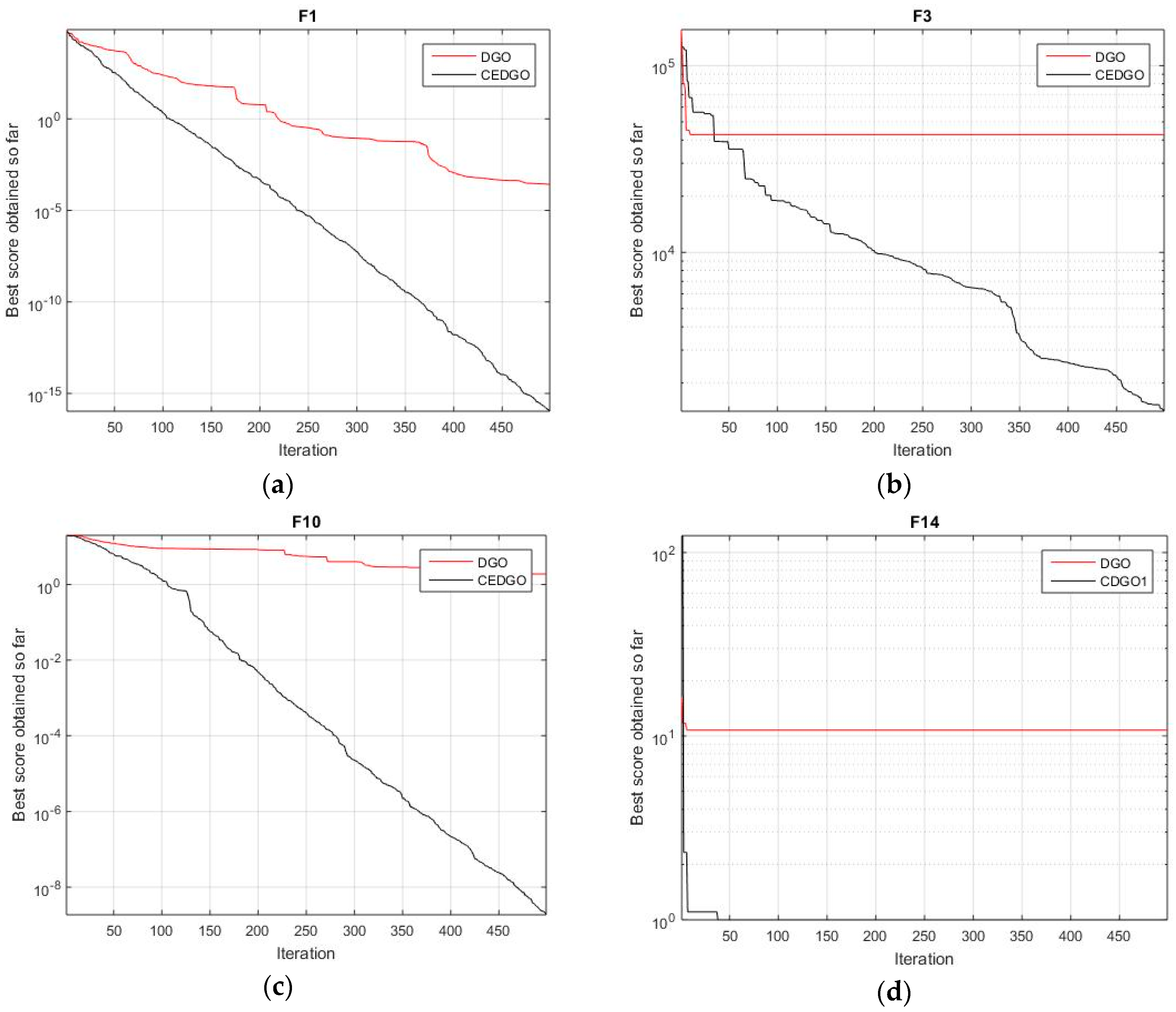
Figure 2.
Diversity of DGO and CEDGO at dimension 10, 30, and 50.

Table 1.
The diversity of dynamic group optimizations (DGOs) at different dimensions.
| D = 10 | D = 30 | D = 50 | |
|---|---|---|---|
| DGO | 0.0261 | 0.0852 | 0.1577 |
| inDGO | 0.542 | 0.1221 | 0.3747 |
Table 2.
The diversity of DGOs at different dimensions.
| D = 10 | D = 30 | D = 50 | |
|---|---|---|---|
| DGO | 0.0261 | 0.0852 | 0.1577 |
| inDGO | 0.542 | 0.1221 | 0.3747 |
| CEDGO | 0.84402 | 0.4485 | 0.6667 |
Table 3.
Computational environment used for performance experiments.
| Property | Value |
|---|---|
| CPU | Intel i7, 3.60 GHz |
| RAM | 8.00 GB |
| Software | MATLAB R2015a |
Table 4.
Experimental results obtained by the DGO and CEDGO at D = 30.
| Function | DGO | p Value | CEDGO | |
|---|---|---|---|---|
| AVGr ± SDr | AVGr ± SDr | |||
| F1 | 3.68 × 10−133 ± 7.59 × 10−133 | 7.94 × 10−03 | + | 0.00 × 10+00 ± 0.00 × 10+00 |
| F2 | 2.09 × 10⁻¹⁹ ± 4.67 × 10⁻¹⁹ | 7.94 × 10−03 | + | 4.23 × 10−254 ± 0.00 × 10+00 |
| F3 | 5.59 × 10−05 ± 1.25 × 10−04 | 2.22 × 10−03 | + | 3.02 × 10⁻¹⁸ ± 6.64 × 10⁻¹⁸ |
| F4 | 2.29 × 10−02 ± 5.96 × 10−03 | 7.94 × 10−03 | + | 2.92 × 10⁻³⁴ ± 2.71 × 10⁻³⁴ |
| F5 | 1.20 × 10+01 ± 8.96 × 10+00 | 4.21 × 10−01 | = | 6.92 × 10+00 ± 7.76 × 10+00 |
| F6 | 1.83 × 10⁻²² ± 3.44 × 10⁻²² | 7.94 × 10−03 | + | 1.73 × 10⁻³² ± 1.65 × 10⁻³² |
| F7 | 4.85 × 10−03 ± 3.99 × 10−03 | 3.17 × 10−02 | - | 1.61 × 10−02 ± 6.24 × 10−03 |
| F8 | −1.04 × 10+04 ± 3.27 × 10+02 | 2.22 × 10−01 | - | −8.70 × 10+03 ± 2.36 × 10+03 |
| F9 | 3.98 × 10−01 ± 5.45 × 10−01 | 7.94 × 10−03 | - | 9.52 × 10+01 ± 8.43 × 10+01 |
| F10 | 2.07 × 10⁻¹² ± 2.72 × 10⁻¹² | 7.94 × 10−03 | + | 6.57 × 10⁻¹⁵ ± 1.95 × 10⁻¹⁵ |
| F11 | 2.41 × 10−02 ± 1.66 × 10−02 | 3.17 × 10−02 | + | 1.89 × 10−08 ± 2.69 × 10−08 |
| F12 | 1.87 × 10⁻¹⁹ ± 4.19 × 10⁻¹⁹ | 6.51 × 10−01 | = | 1.51 × 10−02 ± 2.07 × 10−02 |
| F13 | 3.31 × 10⁻²¹ ± 5.06 × 10⁻²¹ | 1.35 × 10−01 | = | 2.20 × 10−03 ± 4.91 × 10−03 |
| F14 | 3.74 × 10+00 ± 4.05 × 10+00 | 2.86 × 10−01 | + | 9.98 × 10−01 ± 1.24 × 10⁻¹¹ |
| F15 | 4.34 × 10−03 ± 8.96 × 10−03 | 5.48 × 10−01 | + | 4.95 × 10−04 ± 4.07 × 10−04 |
| F16 | −1.03 × 10+00 ± 0.00 × 10+00 | 1.00 × 10+00 | = | −1.03 × 10+00 ± 0.00 × 10+00 |
| F17 | 3.98 × 10−01 ± 0.00 × 10+00 | 1.00 × 10+00 | = | 3.98 × 10−01 ± 1.04 × 10−07 |
| F18 | 3.00 × 10+00 ± 4.44 × 10⁻¹⁶ | 1.19 × 10−01 | = | 3.00 × 10+00 ± 5.44 × 10⁻¹⁶ |
| F19 | −3.86 × 10+00 ± 0.00 × 10+00 | 1.00 × 10+00 | = | −3.86 × 10+00 ± 2.22 × 10⁻¹⁶ |
| F20 | −3.27 × 10+00 ± 6.51 × 10−02 | 6.83 × 10−01 | = | −3.32 × 10+00 ± 6.51 × 10−02 |
| F21 | −6.13 × 10+00 ± 3.80 × 10+00 | 9.37 × 10−01 | = | −6.62 × 10+00 ± 2.21 × 10+00 |
| F22 | −3.23 × 10+00 ± 1.23 × 10+00 | 7.94 × 10−03 | + | −8.19 × 10+00 ± 2.26 × 10+00 |
| F23 | −3.04 × 10+00 ± 1.18 × 10+00 | 1.59 × 10−02 | + | −8.68 × 10+00 ± 2.24 × 10+00 |
| +/=/- | 11/9/3 | |||
Table 5.
Experimental results obtained by the AGPSO, IPSO, TACPSO, MPSO and CEDGO at D = 30.
| Function | AGPSO | IPSO | TACPSO | MPSO | CEDGO |
|---|---|---|---|---|---|
| AVGr ± SDr | AVGr ± SDr | AVGr ± SDr | AVGr ± SDr | AVGr ± SDr | |
| F1 | 4.39 × 10⁻³¹ ± 9.52 × 10⁻³¹ | 1.34 × 10−73 ± 3.01 × 10−73 | 2.78 × 10−56 ± 6.22 × 10−56 | 1.68 × 10−42 ± 3.75 × 10−42 | 0.00 × 10+00 ± 0.00 × 10+00 |
| F2 | 2.05 × 10⁻¹¹ ± 4.02 × 10⁻¹¹ | 4.00 × 10+00 ± 8.94 × 10+00 | 2.18 × 10⁻¹⁵ ± 3.70 × 10⁻¹⁵ | 3.20 × 10+01 ± 2.49 × 10+01 | 4.23 × 10−254 ± 0.00 × 10+00 |
| F3 | 1.00 × 10+03 ± 2.24 × 10+03 | 2.00 × 10+03 ± 2.74 × 10+03 | 2.56 × 10−09 ± 3.11 × 10−09 | 1.40 × 10+04 ± 5.60 × 10+03 | 3.02 × 10⁻¹⁸ ± 6.64 × 10⁻¹⁸ |
| F4 | 3.48 × 10+00 ± 2.02 × 10+00 | 1.73 × 10−05 ± 1.91 × 10−05 | 6.30 × 10−04 ± 6.83 × 10−04 | 1.81 × 10−02 ± 1.71 × 10−02 | 2.92 × 10⁻³⁴ ± 2.71 × 10⁻³⁴ |
| F5 | 6.15 × 10+02 ± 1.35 × 10+03 | 2.89 × 10+00 ± 2.64 × 10+00 | 1.80 × 10+04 ± 4.02 × 10+04 | 3.60 × 10+04 ± 4.93 × 10+04 | 6.92 × 10+00 ± 7.76 × 10+00 |
| F6 | 2.82 × 10⁻²⁵ ± 6.27 × 10⁻²⁵ | 1.71 × 10⁻³⁰ ± 3.54 × 10⁻³⁰ | 1.43 × 10⁻³⁰ ± 3.10 × 10⁻³⁰ | 8.50 × 10⁻³² ± 1.27 × 10⁻³¹ | 1.73 × 10⁻³² ± 1.65 × 10⁻³² |
| F7 | 4.55 × 10−03 ± 1.02 × 10−03 | 6.36 × 10−03 ± 2.75 × 10−03 | 5.06 × 10−03 ± 3.90 × 10−03 | 1.08 × 10+00 ± 1.47 × 10+00 | 1.61 × 10−02 ± 6.24 × 10−03 |
| F8 | −9.62 × 10+03 ± 5.08 × 10+02 | −9.69 × 10+03 ± 4.64 × 10+02 | −9.91 × 10+03 ± 4.36 × 10+02 | −9.16 × 10+03 ± 8.20 × 10+02 | −8.70 × 10+03 ± 2.36 × 10+03 |
| F9 | 1.53 × 10+01 ± 3.89 × 10+00 | 5.35 × 10+01 ± 2.99 × 10+01 | 3.64 × 10+01 ± 1.09 × 10+01 | 9.52 × 10+01 ± 4.62 × 10+01 | 9.52 × 10+01 ± 8.43 × 10+01 |
| F10 | 7.55 × 10⁻¹⁴ ± 1.13 × 10⁻¹³ | 5.31 × 10−01 ± 7.38 × 10−01 | 8.20 × 10−01 ± 8.51 × 10−01 | 9.75 × 10⁻¹⁴ ± 1.14 × 10⁻¹³ | 6.57 × 10⁻¹⁵ ± 1.95 × 10⁻¹⁵ |
| F11 | 4.96 × 10−02 ± 3.01 × 10−02 | 2.36 × 10−02 ± 3.02 × 10−02 | 2.95 × 10−02 ± 5.65 × 10−02 | 2.01 × 10−02 ± 3.31 × 10−02 | 1.89 × 10−08 ± 2.69 × 10−08 |
| F12 | 2.07 × 10−02 ± 4.64 × 10−02 | 6.22 × 10−02 ± 5.68 × 10−02 | 1.04 × 10−01 ± 2.32 × 10−01 | 2.49 × 10−01 ± 5.01 × 10−01 | 1.51 × 10−02 ± 2.07 × 10−02 |
| F13 | 4.39 × 10−03 ± 6.02 × 10−03 | 2.20 × 10−03 ± 4.91 × 10−03 | 2.39 × 10−02 ± 4.15 × 10−02 | 2.20 × 10−03 ± 4.91 × 10−03 | 2.20 × 10−03 ± 4.91 × 10−03 |
| F14 | 9.98 × 10−01 ± 0.00 × 10+00 | 9.98 × 10−01 ± 0.00 × 10+00 | 9.98 × 10−01 ± 0.00 × 10+00 | 9.98 × 10−01 ± 0.00 × 10+00 | 9.98 × 10−01 ± 1.24 × 10⁻¹¹ |
| F15 | 4.91 × 10−04 ± 4.10 × 10−04 | 3.07 × 10−04 ± 5.41 × 10⁻¹⁹ | 3.07 × 10−04 ± 9.46 × 10⁻¹⁹ | 4.93 × 10−03 ± 8.63 × 10−03 | 4.95 × 10−04 ± 4.07 × 10−04 |
| F16 | −1.03 × 10+00 ± 0.00 × 10+00 | −1.03 × 10+00 ± 0.00 × 10+00 | −1.03 × 10+00 ± 0.00 × 10+00 | −1.03 × 10+00 ± 0.00 × 10+00 | −1.03 × 10+00 ± 0.00 × 10+00 |
| F17 | 3.98 × 10−01 ± 0.00 × 10+00 | 3.98 × 10−01 ± 0.00 × 10+00 | 3.98 × 10−01 ± 0.00 × 10+00 | 3.98 × 10−01 ± 0.00 × 10+00 | 3.98 × 10−01 ± 1.04 × 10−07 |
| F18 | 3.00 × 10+00 ± 9.93 × 10⁻¹⁶ | 3.00 × 10+00 ± 0.00 × 10+00 | 3.00 × 10+00 ± 0.00 × 10+00 | 3.00 × 10+00 ± 0.00 × 10+00 | 3.00 × 10+00 ± 5.44 × 10⁻¹⁶ |
| F19 | −3.86 × 10+00 ± 0.00 × 10+00 | −3.86 × 10+00 ± 0.00 × 10+00 | −3.86 × 10+00 ± 0.00 × 10+00 | −3.86 × 10+00 ± 0.00 × 10+00 | −3.86 × 10+00 ± 2.22 × 10⁻¹⁶ |
| F20 | −3.32 × 10+00 ± 0.00 × 10+00 | −3.30 × 10+00 ± 5.32 × 10−02 | −3.32 × 10+00 ± 0.00 × 10+00 | −3.25 × 10+00 ± 6.64 × 10−02 | −3.32 × 10+00 ± 6.51 × 10−02 |
| F21 | −8.13 × 10+00 ± 2.77 × 10+00 | −8.13 × 10+00 ± 2.77 × 10+00 | −9.14 × 10+00 ± 2.26 × 10+00 | −9.14 × 10+00 ± 2.26 × 10+00 | −6.62 × 10+00 ± 2.21 × 10+00 |
| F22 | −1.04 × 10+01 ± 0.00 × 10+00 | −1.04 × 10+01 ± 1.26 × 10⁻¹⁵ | −9.35 × 10+00 ± 2.36 × 10+00 | −8.29 × 10+00 ± 2.90 × 10+00 | −8.19 × 10+00 ± 2.26 × 10+00 |
| F23 | −1.05 × 10+01 ± 8.88 × 10⁻¹⁶ | −1.05 × 10+01 ± 8.88 × 10⁻¹⁶ | −9.46 × 10+00 ± 2.40 × 10+00 | −1.05 × 10+01 ± 8.88 × 10⁻¹⁶ | −8.68 × 10+00 ± 2.24 × 10+00 |
Table 6.
Parameters setting.
| Algorithm | Parameter Setting |
|---|---|
| BA | P = 30, loudness = 0.5, pulse rate = 0.5 |
| WSA | P = 30, pa = 0.25 |
| PSO | P = 30, c1 = 1.49, c2 = 1.49 |
| GA | P = 30, Cr = 0.8, Mr = 0.2 |
Table 7.
Experimental results obtained by the BA, PSO, GA, WSA and CEDGO at D = 30.
| Function | BA | PSO | GA | WSA | CEDGO |
|---|---|---|---|---|---|
| AVGr ± SDr | AVGr ± SDr | AVGr ± SDr | AVGr ± SDr | AVGr ± SDr | |
| F1 | 1.12 × 10−05 ± 8.86 × 10−07 | 3.67 × 10−158 ± 8.21 × 10−158 | 7.73 × 10⁻¹⁹ ± 2.36 × 10⁻¹⁹ | 2.44 × 10−03 ± 6.51 × 10−04 | 0.00 × 10+00 ± 0.00 × 10+00 |
| F2 | 2.07 × 10+02 ± 2.62 × 10+02 | 1.62 × 10−73 ± 3.62 × 10−73 | 2.60 × 10−08 ± 1.98 × 10−08 | 9.78 × 10+07 ± 1.42 × 10+08 | 4.23 × 10−254 ± 0.00 × 10+00 |
| F3 | 2.92 × 10−05 ± 8.16 × 10−06 | 1.11 × 10−06 ± 1.97 × 10−06 | 4.04 × 10−05 ± 2.55 × 10−05 | 1.58 × 10−02 ± 6.81 × 10−03 | 3.02 × 10⁻¹⁸ ± 6.64 × 10⁻¹⁸ |
| F4 | 1.75 × 10+00 ± 3.97 × 10−01 | 5.26 × 10+00 ± 3.26 × 10+00 | 7.98 × 10−02 ± 1.90 × 10−02 | 1.00 × 10+01 ± 0.00 × 10+00 | 2.92 × 10⁻³⁴ ± 2.71 × 10⁻³⁴ |
| F5 | 7.44 × 10+00 ± 1.16 × 10+00 | 3.33 × 10+02 ± 7.39 × 10+02 | 2.36 × 10+01 ± 6.35 × 10−01 | 1.75 × 10+01 ± 5.42 × 10+00 | 6.92 × 10+00 ± 7.76 × 10+00 |
| F6 | 1.13 × 10−05 ± 8.20 × 10−07 | 6.27 × 10⁻³¹ ± 6.38 × 10⁻³¹ | 5.00 × 10⁻¹⁹ ± 1.54 × 10⁻¹⁹ | 2.31 × 10−03 ± 3.89 × 10−04 | 1.73 × 10⁻³² ± 1.65 × 10⁻³² |
| F7 | 5.63 × 10+00 ± 8.14 × 10−01 | 5.42 × 10+00 ± 8.40 × 10+00 | 2.24 × 10−01 ± 2.29 × 10−02 | 6.73 × 10−03 ± 1.59 × 10−03 | 1.61 × 10−02 ± 6.24 × 10−03 |
| F8 | −8.52 × 10+09 ± 4.57 × 10+07 | −1.23 × 10+03 ± 5.80 × 10+03 | −7.27 × 10+02 ± 6.14 × 10+01 | −1.34 × 10+02 ± 1.68 × 10+01 | −8.70 × 10+03 ± 2.36 × 10+03 |
| F9 | 2.26 × 10+02 ± 9.35 × 10+01 | 1.71 × 10+02 ± 7.48 × 10+01 | 7.36 × 10+00 ± 3.42 × 10+00 | 4.22 × 10+02 ± 8.93 × 10+01 | 9.52 × 10+01 ± 8.43 × 10+01 |
| F10 | 8.28 × 10+00 ± 1.40 × 10+00 | 2.03 × 10+01 ± 1.75 × 10−01 | 8.81 × 10⁻¹¹ ± 3.67 × 10⁻¹¹ | 1.73 × 10+01 ± 0.00 × 10+00 | 6.57 × 10⁻¹⁵ ± 1.95 × 10⁻¹⁵ |
| F11 | 1.08 × 10−02 ± 6.40 × 10−03 | 5.91 × 10−03 ± 6.18 × 10−03 | 2.22 × 10−07 ± 4.97 × 10⁻¹⁷ | 2.69 × 10−04 ± 5.52 × 10−05 | 1.89 × 10−08 ± 2.69 × 10−08 |
| F12 | 4.15 × 10−02 ± 9.27 × 10−02 | 9.11 × 10−01 ± 1.47 × 10+00 | 2.07 × 10−02 ± 4.64 × 10−02 | 1.11 × 10+02 ± 2.70 × 10−02 | 1.51 × 10−02 ± 2.07 × 10−02 |
| F13 | 9.46 × 10+00 ± 5.65 × 10+00 | 1.76 × 10+00 ± 1.80 × 10+00 | 1.54 × 10−02 ± 1.67 × 10−02 | 4.18 × 10+00 ± 1.96 × 10+00 | 2.20 × 10−03 ± 4.91 × 10−03 |
| F14 | 1.17 × 10+01 ± 2.15 × 10+00 | 1.20 × 10+00 ± 4.45 × 10−01 | 0.00 × 10+00 ± 2.10 × 10+00 | 1.74 × 10+01 ± 4.55 × 10+00 | 9.98 × 10−01 ± 1.24 × 10⁻¹¹ |
| F15 | 2.95 × 10−02 ± 5.89 × 10−02 | 1.33 × 10−03 ± 4.20 × 10−04 | 1.15 × 10−03 ± 3.86 × 10−04 | 3.07 × 10−04 ± 1.48 × 10−05 | 4.95 × 10−04 ± 4.07 × 10−04 |
| F16 | −8.68 × 10−01 ± 3.65 × 10−01 | −1.03 × 10+00 ±1.92 × 10⁻¹⁶ | −1.03 × 10+00 ± 1.11 × 10⁻¹⁶ | −1.03 × 10+00 ± 2.53 × 10⁻¹⁰ | −1.03 × 10+00 ± 0.00 × 10+00 |
| F17 | 3.98 × 10−01 ± 2.29 × 10⁻¹¹ | 3.98 × 10−01 ± 0.00 × 10+00 | 3.98 × 10−01 ± 0.00 × 10+00 | −1.03 × 10+00 ± 1.82 × 10⁻¹⁰ | 3.98 × 10−01 ± 1.04 × 10−07 |
| F18 | 8.40 × 10+00 ± 1.21 × 10+01 | 2.46 × 10+01 ± 3.52 × 10+01 | 1.92 × 10+01 ± 3.62 × 10+01 | 3.00 × 10+00 ± 1.00 × 10−08 | 3.00 × 10+00 ± 5.44 × 10⁻¹⁶ |
| F19 | −3.29 × 10+00 ± 1.28 × 10+00 | −7.73 × 10−01 ± 1.73 × 10+00 | −3.86 × 10+00 ± 3.14 × 10⁻¹⁶ | −3.86 × 10+00 ± 2.09 × 10+00 | −3.86 × 10+00 ± 2.22 × 10⁻¹⁶ |
| F20 | −3.27 × 10+00 ± 6.51 × 10−02 | 0.00 × 10+00 ± 0.00 × 10+00 | −3.25 × 10+00 ± 6.51 × 10−02 | −3.32 × 10+00 ± 0.00 × 10+00 | −3.32 × 10+00 ± 6.51 × 10−02 |
| F21 | −5.12 × 10+00 ± 3.06 × 10+00 | −6.57 × 10+00 ± 3.38 × 10+00 | −4.58 × 10+00 ± 1.06 × 10+00 | −5.67 × 10+00 ± 2.62 × 10−03 | −6.62 × 10+00 ± 2.21 × 10+00 |
| F22 | −7.82 × 10+00 ± 3.64 × 10+00 | −4.76 × 10+00 ± 3.32 × 10+00 | −6.28 × 10+00 ± 3.88 × 10+00 | −7.35 × 10+00 ± 3.94 × 10−03 | −8.19 × 10+00 ± 2.26 × 10+00 |
| F23 | −4.09 × 10+00 ± 3.63 × 10+00 | −4.27 × 10+00 ± 3.59 × 10+00 | −8.37 × 10+00 ± 2.96 × 10+00 | −7.29 × 10+00 ± 2.00 × 10−04 | −8.68 × 10+00 ± 2.24 × 10+00 |
Table 8.
Experimental results obtained by the BA, PSO, GA, WSA, DGO and CEDGO at D = 300.
| Function | GA | PSO | BA | WSA | DGO | CEDGO |
|---|---|---|---|---|---|---|
| AVGr ± SDr | AVGr ± SDr | AVGr ± SDr | AVGr ± SDr | AVGr ± SDr | AVGr ± SDr | |
| F1 | 1.87 × 10−03 ± 3.05 × 10−04 | 5.04 × 10+05 ± 3.47 × 10+05 | 1.66 × 10−03 ± 5.61 × 10−05 | 1.59 × 10+00 ± 4.46 × 10−02 | 9.71 × 10−04 ± 1.56 × 10−05 | 3.93 × 10⁻²⁸ ± 4.17 × 10⁻²⁸ |
| F2 | 2.83 × 10+01 ± 2.75 × 10+00 | - | 5.63 × 10+00 ± 1.18 × 10+00 | 4.43 × 10+21 ± 1.49 × 10+22 | 1.69 × 10−01 ± 3.07 × 10−01 | 1.44 × 10⁻¹⁷ ± 3.21 × 10⁻¹⁷ |
| F3 | 3.09 × 10+02 ± 2.11 × 10+02 | 4.53 × 10+07 ± 1.10 × 10+07 | 6.42 × 10+00 ± 2.86 × 10+00 | 4.95 × 10+03 ± 3.83 × 10+02 | 1.89 × 10+05 ± 1.13 × 10+05 | 9.36 × 10+05 ± 1.81 × 10+05 |
| F4 | 2.09 × 10+00 ± 1.66 × 10−01 | 7.55 × 10+02 ± 5.15 × 10+01 | 8.63 × 10−01 ± 1.25 × 10−01 | 2.00 × 10+00 ± 0.00 × 10+00 | 6.88 × 10+00 ± 3.35 × 10+00 | 9.83 × 10+01 ± 4.34 × 10−01 |
| F5 | 5.33 × 10+02 ± 8.41 × 10+01 | 1.47 × 10+13 ± 3.25 × 10+13 | 2.95 × 10+02 ± 1.45 × 10+00 | 8.58 × 10+02 ± 2.44 × 10+01 | 8.36 × 10+01 ± 1.78 × 10+01 | 3.63 × 10+02 ± 5.59 × 10+01 |
| F6 | 1.97 × 10−03 ± 4.18 × 10−04 | 4.43 × 10+05 ± 3.13 × 10+05 | 1.67 × 10−03 ± 5.81 × 10−05 | 1.62 × 10+00 ± 4.16 × 10−02 | 5.80 × 10−04 ± 4.80 × 10−03 | 2.31 × 10⁻²⁸ ± 6.93 × 10⁻²⁹ |
| F7 | 4.01 × 10+00 ± 5.19 × 10−01 | 3.16 × 10+13 ± 1.11 × 10+14 | 5.39 × 10+00 ± 6.79 × 10−01 | 8.29 × 10+00 ± 6.21 × 10−01 | 1.40 × 10+00 ± 3.70 × 10−01 | 8.49 × 10−01 ± 3.56 × 10−01 |
| F8 | −5.62 × 10+03 ± 1.69 × 10+03 | - | - | −1.21 × 10+03 ± 1.61 × 10+01 | −9.04 × 10+04 ± 2.60 × 10+04 | −3.74 × 10+04 ± 1.53 × 10+04 |
| F9 | 2.89 × 10+02 ± 4.93 × 10+01 | 7.58 × 10+05 ± 4.84 × 10+05 | 3.34 × 10+02 ± 1.49 × 10+02 | 1.20 × 10+03 ± 0.00 × 10+00 | 9.60 × 10+01 ± 1.75 × 10+01 | 2.23 × 10+03 ± 3.12 × 10+02 |
| F10 | 2.86 × 10+00 ± 1.47 × 10−01 | 2.11 × 10+01 ± 2.97 × 10−01 | 2.17 × 10+00 ± 2.50 × 10−01 | 6.59 × 10+00 ± 9.11 × 10⁻¹⁶ | 1.94 × 10+00 ± 2.35 × 10+00 | 1.78 × 10+00 ± 8.06 × 10−01 |
| F11 | 1.64 × 10−03 ± 2.14 × 10−03 | 1.30 × 10+02 ± 1.18 × 10+02 | 1.80 × 10−05 ± 1.29 × 10−06 | 2.14 × 10−02 ± 9.15 × 10−04 | 1.70 × 10−05 ± 1.86 × 10−06 | 1.48 × 10−03 ± 3.31 × 10−03 |
| F12 | 1.09 × 10−03 ± 3.21 × 10−03 | 4.69 × 10+13 ± 1.76 × 10+14 | 2.07 × 10−03 ± 5.42 × 10−03 | 2.99 × 10+00 ± 1.98 × 10−01 | 1.11 × 10−04 ± 2.45 × 10−05 | 4.20 × 10+06 ± 4.67 × 10+06 |
| F13 | 1.05 × 10+01 ± 2.47 × 10+00 | 1.02 × 10+13 ± 1.57 × 10+13 | 1.55 × 10+01 ± 5.58 × 10+00 | 3.00 × 10+01 ± 0.00 × 10+00 | 1.21 × 10+00 ± 2.03 × 10+00 | 4.88 × 10+05 ± 7.71 × 10+05 |
Table 9.
Experimental results obtained by Different Lr at D = 30.
| Function | 0.25 | 0.5 | 0.65 | 0.8 |
|---|---|---|---|---|
| AVGr ± SDr | AVGr ± SDr | AVGr ± SDr | AVGr ± SDr | |
| F1 | 4.04 × 10−05 ± 9.04 × 10−05 | 4.61 × 10−07 ± 9.17 × 10−07 | 3.63 × 10⁻²⁸ ± 8.04 × 10⁻²⁸ | 0.00 × 10+00 ± 0.00 × 10+00 |
| F2 | 8.96 × 10−09 ± 1.38 × 10−08 | 2.91 × 10−05 ± 6.50 × 10−05 | 1.83 × 10⁻²⁷ ± 4.04 × 10⁻²⁷ | 7.54 × 10−221 ± 0.00 × 10+00 |
| F3 | 4.73 × 10−02 ± 3.69 × 10−02 | 1.30 × 10+00 ± 2.88 × 10+00 | 2.02 × 10+02 ± 4.35 × 10+02 | 7.07 × 10+01 ± 1.23 × 10+02 |
| F4 | 3.32 × 10−03 ± 4.85 × 10−03 | 6.92 × 10−02 ± 1.55 × 10−01 | 4.16 × 10+00 ± 4.49 × 10+00 | 5.59 × 10⁻³⁰ ± 1.21 × 10⁻²⁹ |
| F5 | 2.74 × 10+01 ± 1.30 × 10+00 | 2.65 × 10+01 ± 1.68 × 10+00 | 1.36 × 10+02 ± 1.01 × 10+02 | 1.26 × 10+01 ± 2.74 × 10+01 |
| F6 | 2.29 × 10+00 ± 1.14 × 10+00 | 3.70 × 10−01 ± 3.89 × 10−01 | 2.47 × 10−03 ± 3.70 × 10−03 | 2.47 × 10⁻³⁴ ± 1.95 × 10⁻³⁴ |
| F7 | 3.92 × 10−04 ± 3.60 × 10−04 | 2.60 × 10−03 ± 1.14 × 10−03 | 1.00 × 10−02 ± 4.45 × 10−03 | 1.61 × 10−02 ± 9.23 × 10−03 |
| F8 | −6.29 × 10+03 ± 7.21 × 10+02 | −7.37 × 10+03 ± 3.95 × 10+02 | −9.37 × 10+03 ± 8.64 × 10+02 | −7.25 × 10+03 ± 2.15 × 10+03 |
| F9 | 1.15 × 10+02 ± 3.47 × 10+01 | 9.67 × 10+01 ± 2.66 × 10+01 | 6.41 × 10+01 ± 2.44 × 10+01 | 1.19 × 10+02 ± 4.93 × 10+01 |
| F10 | 2.19 × 10⁻¹¹ ± 1.99 × 10⁻¹¹ | 2.74 × 10−03 ± 6.12 × 10−03 | 4.44 × 10⁻¹⁵ ± 0.00 × 10+00 | 5.86 × 10⁻¹⁵ ± 1.95 × 10⁻¹⁵ |
| F11 | 2.58 × 10⁻¹⁵ ± 5.76 × 10⁻¹⁵ | 8.10 × 10−03 ± 1.78 × 10−02 | 6.23 × 10−02 ± 1.39 × 10−01 | 3.30 × 10−05 ± 7.08 × 10−05 |
| F12 | 1.03 × 10−01 ± 5.93 × 10−02 | 1.93 × 10−02 ± 2.68 × 10−02 | 3.40 × 10−01 ± 6.64 × 10−01 | 1.13 × 10⁻³² ± 3.53 × 10⁻³⁴ |
| F13 | 2.04 × 10+00 ± 3.12 × 10−01 | 9.08 × 10−01 ± 6.49 × 10−01 | 1.22 × 10−01 ± 2.61 × 10−01 | 4.39 × 10−03 ± 6.02 × 10−03 |
| F14 | 9.98 × 10−01 ± 7.70 × 10⁻¹⁰ | 9.98 × 10−01 ± 9.28 × 10⁻¹⁰ | 9.98 × 10−01 ± 1.11 × 10⁻¹⁶ | 9.98 × 10−01 ± 2.22 × 10⁻¹⁶ |
| F15 | 3.33 × 10−04 ± 5.24 × 10−05 | 7.79 × 10−04 ± 4.29 × 10−04 | 4.31 × 10−04 ± 1.59 × 10−04 | 6.84 × 10−04 ± 5.13 × 10−04 |
| F16 | −1.03 × 10+00 ± 0.00 × 10+00 | −1.03 × 10+00 ± 1.11 × 10⁻¹⁶ | −1.03 × 10+00 ± 0.00 × 10+00 | −1.03 × 10+00 ± 6.15 × 10−09 |
| F17 | 3.98 × 10−01 ± 3.18 × 10⁻¹² | 3.98 × 10−01 ± 6.12 × 10−06 | 3.98 × 10−01 ± 3.56 × 10−06 | 3.98 × 10−01± 7.42 × 10−05 |
| F18 | 3.00 × 10+00 ± 6.51 × 10−08 | 3.00 × 10+00 ± 1.75 × 10⁻¹⁵ | 3.00 × 10+00 ± 2.01 × 10⁻¹⁵ | 3.00 × 10+00 ± 1.02 × 10⁻¹⁵ |
| F19 | −3.86 × 10+00 ± 7.02 × 10−05 | −3.86 × 10+00 ± 0.00 × 10+00 | −3.86 × 10+00 ± 0.00 × 10+00 | −3.86 × 10+00 ± 0.00 × 10+00 |
| F20 | −3.27 × 10+00 ± 6.47 × 10−02 | −3.32 × 10+00 ± 1.17 × 10−05 | −3.25 × 10+00 ± 6.51 × 10−02 | −3.27 × 10+00 ± 6.51 × 10−02 |
| F21 | −7.91 × 10+00 ± 2.62 × 10+00 | −8.19 × 10+00 ± 2.28 × 10+00 | −6.40 × 10+00 ± 2.69 × 10+00 | −7.20 × 10+00 ± 2.96 × 10+00 |
| F22 | −9.08 × 10+00 ± 2.24 × 10+00 | −8.55 × 10+00 ± 1.16 × 10+00 | −7.47 × 10+00 ± 2.93 × 10+00 | −8.80 × 10+00 ± 1.94 × 10+00 |
| F23 | −9.18 × 10+00 ± 2.27 × 10+00 | −9.93 × 10+00 ± 8.52 × 10−01 | −6.93 × 10+00 ± 1.83 × 10+00 | −9.06 × 10+00 ± 1.65 × 10+00 |
Table 10.
Experimental results obtained by ACODE, CODE, jDE, SaDE, and CEDGO at D = 300.
| ACODE | CODE | jDE | SaDE | CEDGO | |
|---|---|---|---|---|---|
| F1 | 0.00 × 10+00 ± 0.00 × 10+00 | 0.00 × 10+00 ± 0.00 × 10+00 | 0.00 × 10+00 ± 0.00 × 10+00 | 0.00 × 10+00 ± 0.00 × 10+00 | 0.00 × 10+00 ± 0.00 × 10+00 |
| F2 | 0.00 × 10+00 ± 0.00 × 10+00 | 0.00 × 10+00 ± 0.00 × 10+00 | 0.00 × 10+00 ± 0.00 × 10+00 | 4.87 × 10−104 ± 2.11 × 10−103 | 4.23 × 10−254 ± 0.00 × 10+00 |
| F3 | 4.60 × 10⁻¹⁷ ± 6.85 × 10⁻¹⁷ | 6.24 × 10⁻¹⁶ ± 1.79 × 10⁻¹⁵ | 1.38 × 10⁻¹² ± 3.74 × 10⁻¹² | 3.74 × 10−06 ± 6.45 × 10−06 | 3.02 × 10⁻¹⁸ ± 6.64 × 10⁻¹⁸ |
| F4 | 8.34 × 10⁻¹⁸ ± 5.55 × 10⁻¹⁸ | 7.81 × 10⁻¹⁶ ± 6.52 × 10⁻¹⁶ | 1.81 × 10+01 ± 6.48 × 10+00 | 5.51 × 10−05 ± 2.35 × 10−04 | 2.92 × 10⁻³⁴ ± 2.71 × 10⁻³⁴ |
| F5 | 3.99 × 10−01 ± 1.23 × 10+00 | 3.43 × 10⁻¹¹ ± 9.25 × 10⁻¹¹ | 9.97 × 10−01 ± 1.77 × 10+00 | 2.49 × 10+01 ± 2.42 × 10+01 | 6.92 × 10+00 ± 7.76 × 10+00 |
| F6 | 0.00 × 10+00 ± 0.00 × 10+00 | 0.00 × 10+00 ± 0.00 × 10+00 | 5.24 × 10⁻³³ ± 8.25 × 10⁻³³ | 1.08 × 10⁻³³ ± 1.08 × 10⁻³³ | 1.73 × 10⁻³² ± 1.65 × 10⁻³² |
| F7 | 2.30 × 10−03 ± 8.57 × 10−04 | 2.70 × 10−03 ± 7.69 × 10−04 | 2.85 × 10−03 ± 2.95 × 10−03 | 4.70 × 10−03 ± 1.90 × 10−03 | 1.61 × 10−02 ± 6.24 × 10−03 |
| F8 | −1.26 × 10+04 ± 1.87 × 10⁻¹² | −1.26 × 10+04 ± 1.87 × 10⁻¹² | −1.25 × 10+04 ± 9.80 × 10+01 | −1.26 × 10+04 ± 2.65 × 10+01 | −8.70 × 10+03 ± 2.36 × 10+03 |
| F9 | 0.00 × 10+00 ± 0.00 × 10+00 | 4.97 × 10−-02± 2.23 × 10−01 | 1.49 × 10−01 ± 3.65 × 10−01 | 7.96 × 10−01 ± 8.90 × 10−01 | 9.52 × 10+01 ± 8.43 × 10+01 |
| F10 | 4.44 × 10⁻¹⁵ ± 0.00 × 10+00 | 4.44 × 10⁻¹⁵ ± 0.00 × 10+00 | 1.24 × 10⁻¹⁴ ± 1.59 × 10⁻¹⁴ | 1.09 × 10+00 ± 7.21 × 10−01 | 6.57 × 10⁻¹⁵ ± 1.95 × 10⁻¹⁵ |
| F11 | 0.00 × 10+00 ± 0.00 × 10+00 | 0.00 × 10+00 ± 0.00 × 10+00 | 4.06 × 10−03 ± 8.89 × 10−03 | 1.04 × 10−02 ± 1.69 × 10−02 | 1.89 × 10−08 ± 2.69 × 10−08 |
| F12 | 1.57 × 10⁻³² ± 2.81 × 10−48 | 1.57 × 10⁻³² ± 2.81 × 10−48 | 6.80 × 10−02 ± 2.80 × 10−01 | 6.22 × 10−02 ± 1.63 × 10−01 | 1.51 × 10−02 ± 2.07 × 10−02 |
| F13 | 1.35 × 10⁻³² ± 2.81 × 10−48 | 1.35 × 10⁻³² ± 2.81 × 10−48 | 5.49 × 10−04 ± 2.46 × 10−03 | 7.99 × 10−02 ± 7.99 × 10−02 | 2.20 × 10-03 ± 4.91 × 10−03 |
| F14 | 9.98 × 10−01 ± 0.00 × 10+00 | 9.98 × 10−01± 5.09 × 10⁻¹⁷ | 1.05 × 10+00 ± 2.22 × 10−01 | 9.98 × 10−01 ± 0.00 × 10+00 | 9.98 × 10−01 ± 1.24 × 10⁻¹¹ |
| F15 | 3.07 × 10−04 ±1.03 × 10⁻¹⁹ | 3.07 × 10−04 ± 1.27 × 10⁻¹⁹ | 3.07 × 10−04 ± 1.09 × 10⁻¹⁹ | 3.07 × 10−04 ± 9.79 × 10⁻²⁰ | 4.95 × 10−04 ± 4.07 × 10−04 |
| F16 | −1.03 × 10+00 ± 2.10 × 10⁻¹⁶ | −1.03 × 10+00 ± 2.04 × 10⁻¹⁶ | −1.03 × 10+00 ± 2.28 × 10⁻¹⁶ | −1.03 × 10+00 ± 2.28 × 10⁻¹⁶ | −1.03 × 10+00 ± 0.00 × 10+00 |
| F17 | 3.98 × 10−01 ± 0.00 × 10+00 | 3.98 × 10−01 ± 0.00 × 10+00 | −1.03 × 10+00 ± 2.28 × 10⁻¹⁶ | 3.98 × 10−01 ± 0.00 × 10+00 | 3.98 × 10−01 ± 1.04 × 10−07 |
| F18 | 3.00 × 10+00 ± 9.77 × 10⁻¹⁶ | 3.00 × 10+00 ± 9.11 × 10⁻¹⁶ | 3.00 × 10+00 ± 7.42 × 10⁻¹⁶ | 3.00 × 10+00 ± 2.04 × 10⁻¹⁶ | 3.00 × 10+00 ± 5.44 × 10⁻¹⁶ |
| F19 | −3.86 × 10+00 ± 2.28 × 10⁻¹⁵ | −3.86 × 10+00 ± 2.28 × 10⁻¹⁵ | −3.86 × 10+00 ± 2.28 × 10⁻¹⁵ | −3.86 × 10+00 ± 2.28 × 10⁻¹⁵ | −3.86 × 10+00 ± 2.22 × 10⁻¹⁶ |
| F20 | −3.32 × 10+00 ± 5.49 × 10⁻¹⁶ | −3.31 × 10+00 ± 3.66 × 10−02 | −3.29 × 10+00 ± 5.59 × 10−02 | −3.32 × 10+00 ± 6.98 × 10⁻¹⁶ | −3.32 × 10+00 ± 6.51 × 10−02 |
| F21 | −1.02 × 10+01 ± 3.51 × 10⁻¹⁵ | −1.02 × 10+01 ± 3.58 × 10⁻¹⁵ | −9.53 × 10+00 ± 1.97 × 10+00 | −9.90 × 10+00 ± 1.13 × 10+00 | −6.62 × 10+00 ± 2.21 × 10+00 |
| F22 | −1.04 × 10+01 ± 3.05 × 10⁻¹⁵ | −1.04 × 10+01± 3.05 × 10⁻¹⁵ | −1.04 × 10+01 ± 2.41 × 10⁻¹⁵ | −1.01 × 10+01 ± 1.18 × 10+00 | −8.19 × 10+00 ± 2.26 × 10+00 |
| F23 | −1.05 × 10+01 ± 1.78 × 10⁻¹⁵ | −1.05 × 10+01 ± 1.82 × 10⁻¹⁵ | −1.01 × 10+01 ± 1.81 × 10+00 | −1.05 × 10+01 ± 1.95 × 10⁻¹⁵ | −8.68 × 10+00 ± 2.24 × 10+00 |
© 2017 by the authors. Licensee MDPI, Basel, Switzerland. This article is an open access article distributed under the terms and conditions of the Creative Commons Attribution (CC BY) license (http://creativecommons.org/licenses/by/4.0/).
Share and Cite
MDPI and ACS Style
Tang, R.; Fong, S.; Dey, N.; Wong, R.K.; Mohammed, S. Cross Entropy Method Based Hybridization of Dynamic Group Optimization Algorithm. Entropy 2017, 19, 533. https://doi.org/10.3390/e19100533
AMA Style
Tang R, Fong S, Dey N, Wong RK, Mohammed S. Cross Entropy Method Based Hybridization of Dynamic Group Optimization Algorithm. Entropy. 2017; 19(10):533. https://doi.org/10.3390/e19100533
Chicago/Turabian StyleTang, Rui, Simon Fong, Nilanjan Dey, Raymond K. Wong, and Sabah Mohammed. 2017. "Cross Entropy Method Based Hybridization of Dynamic Group Optimization Algorithm" Entropy 19, no. 10: 533. https://doi.org/10.3390/e19100533
Note that from the first issue of 2016, this journal uses article numbers instead of page numbers. See further details here.