Article

Upper Bounds for the Rate Distortion Function of Finite-Length Data Blocks of Gaussian WSS Sources

by
Jesús Gutiérrez-Gutiérrez
*,
Marta Zárraga-Rodríguez
and
Xabier Insausti
Tecnun, University of Navarra, Manuel Lardizábal 13, 20018 San Sebastián, Spain
*
Author to whom correspondence should be addressed.
Entropy 2017, 19(10), 554; https://doi.org/10.3390/e19100554
Submission received: 19 September 2017 / Revised: 14 October 2017 / Accepted: 15 October 2017 / Published: 19 October 2017
(This article belongs to the Special Issue Rate-Distortion Theory and Information Theory)

Abstract

:
In this paper, we present upper bounds for the rate distortion function (RDF) of finite-length data blocks of Gaussian wide sense stationary (WSS) sources and we propose coding strategies to achieve such bounds. In order to obtain those bounds, we previously derive new results on the discrete Fourier transform (DFT) of WSS processes.

1. Introduction

In [1], Pearl gave an upper bound for the rate distortion function (RDF) of finite-length data blocks of Gaussian wide sense stationary (WSS) sources and proved that such bound tends to the RDF of the source when the size of the data block grows. However, he did not give a coding strategy to achieve his bound for a given block length.
In this paper, we present two new upper bounds for the RDF of finite-length data blocks of Gaussian WSS sources and we propose coding strategies to achieve these two bounds for a given block length. Since our bounds are tighter than the one given by Pearl, they also tend to the RDF of the source when the size of the data block grows. In order to obtain our bounds, we previously derive new results on the discrete Fourier transform (DFT) of WSS processes.
It should be mentioned that our coding strategies allow us to deal with Gaussian WSS sources as if they were memoryless. This fact can be used, for instance, to consider Gaussian WSS sources in [2].
The paper is organized as follows. In Section 2 we set up notation and review the mathematical definitions and results used in the rest of the paper. In Section 3 we obtain several results on the DFT of WSS processes which will be applied in Section 4. Finally, in Section 4 we present two new upper bounds for the RDF of finite-length data blocks of Gaussian WSS sources and we propose coding strategies to achieve such bounds. In this section, we also present a numerical example to illustrate the difference between Pearl’s bound and our bounds.

2. Preliminaries

2.1. Notation

In this paper, N , Z , R , and C denote the set of natural numbers (i.e., the set of positive integers), the set of integer numbers, the set of (finite) real numbers, and the set of (finite) complex numbers, respectively. R n × 1 is the set of all real n-dimensional (column) vectors. I n denotes the n × n identity matrix, stands for conjugate transpose, ⊤ denotes transpose, and λ k ( A ) , k { 1 , , n } , are the eigenvalues of an n × n Hermitian matrix A arranged in decreasing order. E stands for expectation, i is the imaginary unit, and Re and Im denote real and imaginary parts, respectively. If z C , then
z ^ : = Re ( z ) Im ( z ) R 2 × 1
and, if z k C for all k { 1 , , n } , then we denote by z n : 1 the n-dimensional (column) vector given by
z n : 1 : = z n z n 1 z n 2 z 1 .
If x k is a random variable for all k N , we denote by { x k : k N } the corresponding random process.
We finish this subsection by reviewing the concept of square Toeplitz matrix.
Definition 1.
An n × n Toeplitz matrix is an n × n matrix of the form
t 0 t 1 t 2 t 1 n t 1 t 0 t 1 t 2 n t 2 t 1 t 0 t 3 n t n 1 t n 2 t n 3 t 0 ,
where t k C with k { 1 n , , n 1 } .
Consider a function f : R C that is continuous and 2 π -periodic. For every n N , we denote by T n ( f ) the n × n Toeplitz matrix given by
T n ( f ) : = ( t j k ) j , k = 1 n ,
where { t k } k Z is the sequence of Fourier coefficients of f:
t k = 1 2 π 0 2 π f ( ω ) e k ω i d ω k Z .
It should be mentioned that T n ( f ) is Hermitian for all n N if and only if f is a real function (see [3] (Theorem 4.4.1)). Furthermore, in this case, from [3] (Theorem 4.4.2), we have
min ( f ) λ n ( T n ( f ) ) λ 1 ( T n ( f ) ) max ( f ) n N .

2.2. DFT of Real Vectors

In this subsection, we recall a well-known property of the DFT of real vectors.
Lemma 1.
Let n N . Consider x k , y k C for all k { 1 , , n } . Suppose that y n : 1 is the DFT of x n : 1 , i.e.,
y n : 1 = V n * x n : 1 ,
where V n is the n × n Fourier unitary matrix
[ V n ] j , k : = 1 n e 2 π ( j 1 ) ( k 1 ) n i , j , k { 1 , , n } .
Then, the two following assertions are equivalent:
(1) 
x n : 1 R n × 1 .
(2) 
y j = y n j ¯ for all j { 1 , , n 1 } and y n R .

2.3. RDF of Real Gaussian WSS Processes

Kolmogorov gave in [4] the following formula for the rate distortion function (RDF) of a real zero-mean Gaussian n-dimensional vector x :
R x ( D ) = 1 n k = 1 n max 0 , 1 2 ln λ k E x x θ ,
where θ is a real number satisfying
D = 1 n k = 1 n min θ , λ k E x x .
R x ( D ) can be thought of as the minimum rate (measured in nats) at which one must encode (compress) x in order to be able to recover it with a mean square error (MSE) per dimension not larger than D, that is:
E x x ˜ 2 2 n D ,
where x ˜ denotes the estimation of x and · 2 is the spectral norm.
We now review the definition of WSS process with continuous power spectral density (PSD).
Definition 2.
Let f : R R be continuous and 2 π -periodic. A random process { x k : k N } is said to be WSS with PSD f if it has constant mean (i.e., E ( x k 1 ) = E ( x k 2 ) for all k 1 , k 2 N ) and { E x n : 1 x n : 1 * } = { T n ( f ) } .
If { x k : k N } is a real zero-mean Gaussian WSS process with continuous PSD f satisfying min ( f ) > 0 and D ( 0 , min ( f ) ] , then from Equations (1) and (2), we obtain
R x n : 1 ( D ) = 1 2 n k = 1 n ln λ k T n ( f ) D = 1 2 n ln det T n ( f ) D n n N .
We recall that the RDF of the source (process) is given by R ( D ) = lim n R x n : 1 ( D ) .

3. DFT of WSS Processes

In this section, we present several new results on the DFT of WSS processes in one theorem.
Theorem 1.
Consider a WSS process { x k : k N } with continuous PSD f. Let n N and y n : 1 = V n * x n : 1 .
(1) 
If j { 1 , , n } , then
min ( f ) E x j 2 max ( f )
and
min ( f ) E y j 2 max ( f )
(2) 
If the process { x k : k N } is real and j { 1 , , n 1 } with j n 2 then
min ( f ) 2 E Re ( y j ) 2 max ( f ) 2
and
min ( f ) 2 E Im ( y j ) 2 max ( f ) 2 .
Proof. 
(1) Since
E x j 2 = E x n : 1 x n : 1 * n j + 1 , n j + 1 = T n ( f ) n j + 1 , n j + 1 = t 0 = T 1 ( f ) , j { 1 , , n }
from Equation (1), we obtain Equation (4).
Let
C ^ n ( f ) : = V n diag 1 j n ( V n * T n ( f ) V n j , j ) V n * ,
where diag 1 j n ( a j ) = ( a j δ j , k ) j , k = 1 n with δ being the Kronecker delta and a j C for all j { 1 , , n } . As
E y n : 1 y n : 1 * = E V n * x n : 1 x n : 1 * V n * * = V n * E x n : 1 x n : 1 * V n * * = V n * T n ( f ) V n ,
we have
C ^ n ( f ) = V n diag 1 j n [ E y n : 1 y n : 1 * ] j , j V n * .
Hence,
λ j ( C ^ n ( f ) ) : j { 1 , , n } = [ E y n : 1 y n : 1 * ] j , j : j { 1 , , n } = E y j 2 , j { 1 , , n } .
Equation (5) now follows by taking N = 1 in [5] (Lemma 6).
(2) Fix j { 1 , , n 1 } with j n 2 . Since
y j = [ y n : 1 ] n j + 1 , 1 = [ V n * x n : 1 ] n j + 1 , 1 = k = 1 n [ V n * ] n j + 1 , k [ x n : 1 ] k , 1 = k = 1 n [ V n ] k , n j + 1 ¯ [ x n : 1 ] k , 1 = k = 1 n 1 n e 2 π ( k 1 ) ( n j ) n i x n : 1 k , 1 = k = 1 n 1 n e 2 π ( k 1 ) i e 2 π ( k 1 ) j n i x n : 1 k , 1 = k = 1 n 1 n e 2 π ( k 1 ) j n i x n : 1 k , 1 = 1 n k = 1 n cos 2 π ( 1 k ) j n + i sin 2 π ( 1 k ) j n x n k + 1 ,
we obtain
E y j ^ y j ^ = E Re ( y j ) Im ( y j ) Re ( y j ) Im ( y j ) = E Re ( y j ) 2 Re ( y j ) Im ( y j ) Im ( y j ) Re ( y j ) Im ( y j ) 2 = 1 n k 1 , k 2 = 1 n cos 2 π ( 1 k 1 ) j n cos 2 π ( 1 k 2 ) j n E x n k 1 + 1 x n k 2 + 1 cos 2 π ( 1 k 1 ) j n sin 2 π ( 1 k 2 ) j n E x n k 1 + 1 x n k 2 + 1 sin 2 π ( 1 k 1 ) j n cos 2 π ( 1 k 2 ) j n E x n k 1 + 1 x n k 2 + 1 sin 2 π ( 1 k 1 ) j n sin 2 π ( 1 k 2 ) j n E x n k 1 + 1 x n k 2 + 1 = 1 n k 1 , k 2 = 1 n cos 2 π ( 1 k 1 ) j n cos 2 π ( 1 k 2 ) j n t k 1 k 2 cos 2 π ( 1 k 1 ) j n sin 2 π ( 1 k 2 ) j n t k 1 k 2 sin 2 π ( 1 k 1 ) j n cos 2 π ( 1 k 2 ) j n t k 1 k 2 sin 2 π ( 1 k 1 ) j n sin 2 π ( 1 k 2 ) j n t k 1 k 2 .
We begin by proving Equation (6). Applying Equation (10) yields
E Re ( y j ) 2 = 1 n k 1 , k 2 = 1 n cos 2 π ( 1 k 1 ) j n cos 2 π ( 1 k 2 ) j n t k 1 k 2 = 1 n k 1 , k 2 = 1 n cos 2 π ( 1 k 1 ) j n cos 2 π ( 1 k 2 ) j n 1 2 π 0 2 π f ( ω ) e ( k 1 k 2 ) ω i d ω = 1 2 π 0 2 π f ( ω ) 1 n k 1 = 1 n cos 2 π ( 1 k 1 ) j n e k 1 ω i 1 n k 2 = 1 n cos 2 π ( 1 k 2 ) j n e k 2 ω i d ω = 1 2 π 0 2 π f ( ω ) 1 n k 1 = 1 n cos 2 π ( 1 k 1 ) j n e k 1 ω i ¯ 1 n k 2 = 1 n cos 2 π ( 1 k 2 ) j n e k 2 ω i d ω = 1 2 π 0 2 π f ( ω ) 1 n k = 1 n cos 2 π ( 1 k ) j n e k ω i 2 d ω ,
and consequently,
min ( f ) 1 2 π 0 2 π 1 n k = 1 n cos 2 π ( 1 k ) j n e k ω i 2 d ω E Re ( y j ) 2 max ( f ) 1 2 π 0 2 π 1 n k = 1 n cos 2 π ( 1 k ) j n e k ω i 2 d ω .
Observe that to finish the proof of Equation (6), we only need to show that
1 2 π 0 2 π 1 n k = 1 n cos 2 π ( 1 k ) j n e k ω i 2 d ω = 1 2 .
Since
1 2 π 0 2 π e m ω i d ω = 1 , if   m = 0 , 0 , if   m Z \ { 0 } ,
we obtain
1 2 π 0 2 π 1 n k = 1 n cos 2 π ( 1 k ) j n e k ω i 2 d ω = 1 n k 1 , k 2 = 1 n cos 2 π ( 1 k 1 ) j n cos 2 π ( 1 k 2 ) j n 1 2 π 0 2 π e ( k 1 k 2 ) ω i d ω = 1 n k = 1 n cos 2 π ( 1 k ) j n 2 = 1 n k = 1 n 1 sin 2 π ( 1 k ) j n 2 = 1 1 n k = 1 n sin 2 π ( 1 k ) j n 2 .
As e 4 π j n i 1 from the formula for the partial sums of the geometric series (see, e.g., [6] (p. 388)), we have
k = 1 n e 4 π ( k 1 ) j n i = h = 0 n 1 e 4 π h j n i = h = 0 n 1 e 4 π j n i h = 1 e 4 π j n i n 1 e 4 π j n i = 1 e 4 π j i 1 e 4 π j n i = 0 .
Applying (14) and the basic trigonometric formula cos ( 2 x ) = 1 2 sin 2 x (see, e.g., [6] (p. 97)) yields
1 n k = 1 n sin 2 π ( 1 k ) j n 2 = 1 n k = 1 n 1 cos 4 π ( 1 k ) j n 2 = 1 n n 2 1 2 k = 1 n cos 4 π ( k 1 ) j n = 1 2 1 2 n k = 1 n Re e 4 π ( k 1 ) j n i = 1 2 1 2 n Re k = 1 n e 4 π ( k 1 ) j n i = 1 2 ,
and, thus, from Equation (13), we obtain Equation (11), and, therefore, Equation (6) holds.
Finally, we prove Equation (7). From Equation (10), we obtain
E Im ( y j ) 2 = 1 n k 1 , k 2 = 1 n sin 2 π ( 1 k 1 ) j n sin 2 π ( 1 k 2 ) j n t k 1 k 2 = 1 n k 1 , k 2 = 1 n sin 2 π ( 1 k 1 ) j n sin 2 π ( 1 k 2 ) j n 1 2 π 0 2 π f ( ω ) e ( k 1 k 2 ) ω i d ω = 1 2 π 0 2 π f ( ω ) 1 n k 1 = 1 n sin 2 π ( 1 k 1 ) j n e k 1 ω i 1 n k 2 = 1 n sin 2 π ( 1 k 2 ) j n e k 2 ω i d ω = 1 2 π 0 2 π f ( ω ) 1 n k 1 = 1 n sin 2 π ( 1 k 1 ) j n e k 1 ω i ¯ 1 n k 2 = 1 n sin 2 π ( 1 k 2 ) j n e k 2 ω i d ω = 1 2 π 0 2 π f ( ω ) 1 n k = 1 n sin 2 π ( 1 k ) j n e k ω i 2 d ω ,
and, consequently,
min ( f ) 1 2 π 0 2 π 1 n k = 1 n sin 2 π ( 1 k ) j n e k ω i 2 d ω E Im ( y j ) 2 max ( f ) 1 2 π 0 2 π 1 n k = 1 n sin 2 π ( 1 k ) j n e k ω i 2 d ω .
Applying Equations (12) and (15) yields
1 2 π 0 2 π 1 n k = 1 n sin 2 π ( 1 k ) j n e k ω i 2 d ω = 1 n k 1 , k 2 = 1 n sin 2 π ( 1 k 1 ) j n sin 2 π ( 1 k 2 ) j n 1 2 π 0 2 π e ( k 1 k 2 ) ω i d ω = 1 n k = 1 n sin 2 π ( 1 k ) j n 2 = 1 2 ,
and, therefore, Equation (7) holds. ☐

4. Upper Bounds for the RDF of Finite-Length Data Blocks of Gaussian WSS Sources
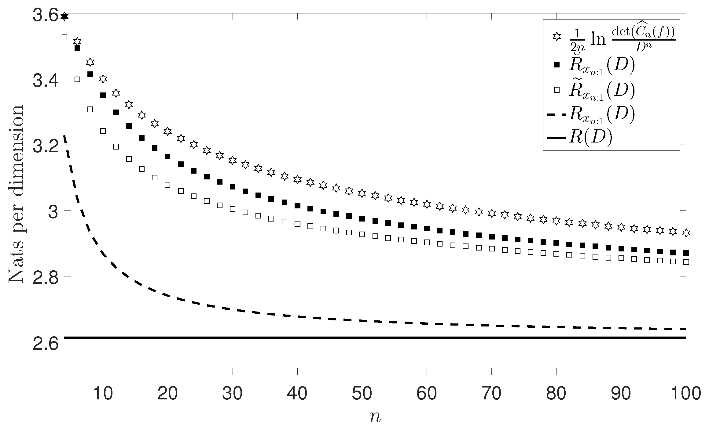
Let { x k : k N } be a real zero-mean Gaussian WSS process with continuous PSD f and min ( f ) > 0 . For a given block length n N and a distortion D ( 0 , min ( f ) ] , Pearl presented in [1] an upper bound of R x n : 1 ( D ) , namely:
1 2 n ln det ( C ^ n ( f ) ) D n ,
where C ^ n ( f ) is the matrix defined in Equation (8). In the following theorem, we give two new upper bounds of R x n : 1 ( D ) , denoted by R ˜ x n : 1 ( D ) and R ˘ x n : 1 ( D ) , that are tighter than the one given by Pearl.
Theorem 2.
Consider a real zero-mean Gaussian WSS process { x k : k N } with continuous PSD f and min ( f ) > 0 . Let D ( 0 , min ( f ) ] . If n N and y n : 1 is the DFT of x n : 1 , then
R x n : 1 ( D ) R ˜ x n : 1 ( D ) R ˘ x n : 1 ( D ) 1 2 n ln det ( C ^ n ( f ) ) D n ,
where R ˜ x n : 1 ( D ) is given by
R ˜ x n : 1 ( D ) = R y n 2 D + 2 k = n 2 + 1 n 1 R y k ^ D 2 + R y n ( D ) n , if   n   is   even , 2 k = n + 1 2 n 1 R y k ^ D 2 + R y n ( D ) n , if   n   is   odd .
and
R ˘ x n : 1 ( D ) = R y n 2 D + k = n 2 + 1 n 1 R Re y k D 2 + R Im y k D 2 + R y n ( D ) n , if   n   is   even , k = n + 1 2 n 1 R Re y k D 2 + R Im y k D 2 + R y n ( D ) n , if   n   is   odd .
Furthermore,
R ( D ) = lim n R x n : 1 ( D ) = lim n R ˜ x n : 1 ( D ) = lim n R ˘ x n : 1 ( D ) = lim n 1 2 n ln det ( C ^ n ( f ) ) D n = 1 4 π 0 2 π ln f ( ω ) D d ω .
Proof. 
We divide the proof into four steps:
Step 1: We show that R x n : 1 ( D ) R ˜ x n : 1 ( D ) . We encode y n 2 , , y n separately with
E y j y j ˜ 2 D
for all j n 2 , , n , where n 2 denotes the smallest integer higher than or equal to n 2 . Observe that if j { n 2 , , n 1 } with j n 2 Equation (19) is equivalent to
E y j ^ y j ˜ ^ 2 2 2 D 2 .
From Lemma 1, y j = y n j ¯ for all j { 1 , , n 2 1 } , and y j R with j { n 2 , n } N . Let x n : 1 ˜ : = V n y n : 1 ˜ , where
y n : 1 ˜ = y n ˜ y 1 ˜ ,
with y j ˜ : = y n j ˜ ¯ for all j { 1 , , n 2 1 } . Applying Lemma 1 yields x n : 1 ˜ R n × 1 .
As V n * is unitary and the spectral norm is unitarily invariant, we have
E x n : 1 x n : 1 ˜ 2 2 n = E V n * x n : 1 V n * x n : 1 ˜ 2 2 n = E y n : 1 V n * V n y n : 1 ˜ 2 2 n = E y n : 1 y n : 1 ˜ 2 2 n = 1 n E j = 1 n y j y j ˜ 2 = 1 n j = 1 n E y j y j ˜ 2 = 1 n j = 1 n 2 1 E y j y j ˜ 2 + k = n 2 n E y k y k ˜ 2 = 1 n j = 1 n 2 1 E y n j ¯ y n j ˜ ¯ 2 + k = n 2 n E y k y k ˜ 2 = 1 n k = n n 2 + 1 n 1 E y k ¯ y k ˜ ¯ 2 + k = n 2 n E y k y k ˜ 2 = 1 n k = n n 2 + 1 n 1 E y k y k ˜ ¯ 2 + k = n 2 n E y k y k ˜ 2 = 1 n k = n n 2 + 1 n 1 E y k y k ˜ 2 + k = n 2 n E y k y k ˜ 2 1 n n 2 1 D + n n 2 + 1 D = D .
Consequently,
R x n : 1 ( D ) R y n 2 D + 2 k = n 2 + 1 n 1 R y k ^ D 2 + R y n ( D ) n , if n is even , 2 k = n + 1 2 n 1 R y k ^ D 2 + R y n ( D ) n , if n is odd .
Step 2: We show that R ˜ x n : 1 ( D ) R ˘ x n : 1 ( D ) . To do that, we only need to prove that
2 R y j ^ D 2 R Re y j D 2 + R Im y j D 2
for all j { n 2 , , n 1 } with j n 2 . Fix j { n 2 , , n 1 } with j n 2 . We encode Re y j and Im y j separately with
E Re ( y j ) Re ( y j ) ˜ 2 D 2
and
E Im ( y j ) Im ( y j ) ˜ 2 D 2 .
Let y j ˜ : = Re ( y j ) ˜ + i Im ( y j ) ˜ . We have
E y j ^ y j ˜ ^ 2 2 2 = E Re ( y j ) Re ( y j ) ˜ 2 + Im ( y j ) Im ( y j ) ˜ 2 2 = 1 2 E Re ( y j ) Re ( y j ) ˜ 2 + E Im ( y j ) Im ( y j ) ˜ 2 1 2 D 2 + D 2 = D 2 .
Consequently,
R y j ^ D 2 R Re y j D 2 + R Im y j D 2 2 .
Step 3: We show that R ˘ x n : 1 ( D ) 1 2 n ln det ( C ^ n ( f ) ) D n . From Equations (2) and (5), we obtain
R y k ( D ) = 1 2 ln E y k 2 D , k n 2 , n N ,
and applying Equations (2), (6) and (7), the arithmetic mean-geometric mean (AM-GM) inequality, and Lemma 1 yields
R Re ( y k ) D 2 + R Im ( y k ) D 2 = 1 2 ln E Re ( y k ) 2 D 2 + 1 2 ln E Im ( y k ) 2 D 2 = 1 2 ln E Re ( y k ) 2 E Im ( y k ) 2 D 2 2 = 1 2 ln E Re ( y k ) 2 E Im ( y k ) 2 2 D 2 2 1 2 ln E Re ( y k ) 2 + E Im ( y k ) 2 2 2 D 2 2 = 1 2 ln E Re ( y k ) 2 + Im ( y k ) 2 2 2 D 2 2 = 1 2 ln E y k 2 2 D 2 = 1 2 ln E y k 2 E y k ¯ 2 D 2 = 1 2 ln E y k 2 E y n k 2 D 2 = 1 2 ln E y k 2 D + ln E y n k 2 D
for all k { n 2 , , n 1 } with k n 2 . Hence, from Equation (9), if n is even, we have
R ˘ x n : 1 ( D ) 1 2 n ln E y n 2 2 D + k = n 2 + 1 n 1 ln E y k 2 D + ln E y n k 2 D + ln E y n 2 D = 1 2 n ln E y n 2 2 D + k = n 2 + 1 n 1 ln E y k 2 D + j = 1 n 2 1 ln E y j 2 D + ln E y n 2 D = 1 2 n k = 1 n ln E y k 2 D = 1 2 n ln k = 1 n E y k 2 D n = 1 2 n ln det ( C ^ n ( f ) ) D n
and, if n is odd,
R ˘ x n : 1 ( D ) 1 2 n k = n + 1 2 n 1 ln E y k 2 D + ln E y n k 2 D + ln E y n 2 D = 1 2 n k = n + 1 2 n 1 ln E y k 2 D + j = 1 n 1 2 ln E y j 2 D + ln E y n 2 D = 1 2 n k = 1 n ln E y k 2 D = 1 2 n ln k = 1 n E y k 2 D n = 1 2 n ln det ( C ^ n ( f ) ) D n
is yielded.
Step 4: We show Equation (18). Applying Equation (3) yields
0 1 2 n ln det ( C ^ n ( f ) ) D n R x n : 1 ( D ) = 1 2 n ln det ( C ^ n ( f ) ) D n 1 2 n ln det T n ( f ) D n = 1 2 n ln det ( C ^ n ( f ) ) det T n ( f ) = 1 2 n ln det ( C ^ n ( f ) ) det ( T n ( f ) ) 1 = 1 2 n ln det ( C ^ n ( f ) ) det T n ( f ) T n ( f ) 1 = 1 2 n ln det ( C ^ n ( f ) ) det T n ( f ) 1 T n ( f ) 1 = 1 2 n ln det ( C ^ n ( f ) ) det T n ( f ) 1 det T n ( f ) 1 = 1 2 n ln det T n ( f ) 1 det ( C ^ n ( f ) ) det T n ( f ) 1 = 1 2 n ln det T n ( f ) 1 C ^ n ( f ) T n ( f ) 1 = 1 2 n ln k = 1 n λ k T n ( f ) 1 C ^ n ( f ) T n ( f ) 1 ,
where T n ( f ) : = U n diag 1 k n λ k ( T n ( f ) ) U n 1 with T n ( f ) = U n diag 1 k n ( λ k ( T n ( f ) ) ) U n 1 being a unitary diagonalization of T n ( f ) . Since T n ( f ) is Hermitian and C ^ n ( f ) is positive definite (see [5] (Lemma 5)), T n ( f ) 1 C ^ n ( f ) T n ( f ) 1 is positive definite, and applying the AM-GM inequality yields
0 1 2 n ln det ( C ^ n ( f ) ) D n R x n : 1 ( D ) 1 2 n ln 1 n k = 1 n λ k T n ( f ) 1 C ^ n ( f ) T n ( f ) 1 n = 1 2 ln 1 n tr T n ( f ) 1 C ^ n ( f ) T n ( f ) 1 = 1 2 ln 1 n tr C ^ n ( f ) T n ( f ) 1 T n ( f ) 1 = 1 2 ln 1 n tr C ^ n ( f ) ( T n ( f ) ) 1 1 2 ln n n C ^ n ( f ) ( T n ( f ) ) 1 F = 1 2 ln 1 n ( C ^ n ( f ) T n ( f ) ) ( T n ( f ) ) 1 + I n F 1 2 ln 1 n ( C ^ n ( f ) T n ( f ) ) ( T n ( f ) ) 1 F + n 1 2 ln 1 n C ^ n ( f ) T n ( f ) F ( T n ( f ) ) 1 2 + n = 1 2 ln T n ( f ) C ^ n ( f ) F n 1 λ n ( T n ( f ) ) + 1 1 2 ln 1 + 1 min ( f ) T n ( f ) C ^ n ( f ) F n ,
where tr stands for trace and · F is the Frobenius norm. From [5] (Lemma 4), we obtain
lim n 1 2 ln 1 + 1 min ( f ) T n ( f ) C ^ n ( f ) F n = 0
and, therefore,
lim n 1 2 n ln det ( C ^ n ( f ) ) D n R x n : 1 ( D ) = 0 .
Consequently, applying [7] (Theorem 5), we conclude that
lim n 1 2 n ln det ( C ^ n ( f ) ) D n = lim n R x n : 1 ( D ) = lim n 1 2 n ln det ( T n ( f ) ) D n = 1 2 lim n 1 n ln k = 1 n λ k ( T n ( f ) ) D = 1 2 lim n 1 n k = 1 n ln λ k T n ( f ) D = 1 4 π 0 2 π ln f ( ω ) D d ω .
As an example, Figure 1 shows Equation (16) for the case in which f ( ω ) = 0.1 + ( ω π ) 6 with ω [ 0 , 2 π ] , D = min ( f ) 2 = 0.05 , and n 100 .
Finally, observe that Theorem 2 also provides coding strategies to achieve the two new bounds of R x n : 1 ( D ) presented: R ˜ x n : 1 ( D ) and R ˘ x n : 1 ( D ) . Specifically, Theorem 2 shows that R ˜ x n : 1 ( D ) can be achieved by encoding y k separately, with k { n 2 , , n } , instead of encoding x n : 1 jointly, and that R ˘ x n : 1 ( D ) can be achieved by encoding separately the real part and the imaginary part of y k instead of encoding y k when k { n 2 , n } . Therefore, although R ˜ x n : 1 ( D ) is a tighter bound, the coding strategy associated with R ˘ x n : 1 ( D ) is simpler. It should be mentioned that, in order to achieve R ˜ x n : 1 ( D ) and R ˘ x n : 1 ( D ) , an optimal coding method of Gaussian random variables is required.

Acknowledgments

This work was supported in part by the Spanish Ministry of Economy and Competitiveness through the CARMEN project (TEC2016-75067-C4-3-R).

Author Contributions

Authors are listed in order of their degree of involvement in the work, with the most active contributors listed first. All authors have read and approved the final manuscript.

Conflicts of Interest

The authors declare no conflict of interest.

References

  1. Pearl, J. On coding and filtering stationary signals by discrete Fourier transforms. IEEE Trans. Inf. Theory 1973, 19, 229–232. [Google Scholar] [CrossRef]
  2. Du, J.; Médard, M.; Xiao, M.; Skoglund, M. Scalable capacity bounding models for wireless networks. IEEE Trans. Inf. Theory 2016, 62, 208–229. [Google Scholar]
  3. Gutiérrez-Gutiérrez, J.; Crespo, P.M. Block Toeplitz matrices: Asymptotic results and applications. Found. Trends Commun. Inf. Theory 2011, 8, 179–257. [Google Scholar]
  4. Kolmogorov, A.N. On the Shannon theory of information transmission in the case of continuous signals. IRE Trans. Inf. Theory 1956, 2, 102–108. [Google Scholar] [CrossRef]
  5. Gutiérrez-Gutiérrez, J.; Zárraga-Rodríguez, M.; Insausti, X.; Hogstad, B.O. On the complexity reduction of coding WSS vector processes by using a sequence of block circulant matrices. Entropy 2017, 19, 95. [Google Scholar]
  6. Apostol, T.M. Calculus; Wiley: New York, NY, USA, 1967; Volume I. [Google Scholar]
  7. Gutiérrez-Gutiérrez, J.; Crespo, P.M. Asymptotically equivalent sequences of matrices and Hermitian block Toeplitz matrices with continuous symbols: Applications to MIMO systems. IEEE Trans. Inf. Theory 2008, 54, 5671–5680. [Google Scholar]
Figure 1. Numerical example of the upper bounds presented in Theorem 2.
Entropy 19 00554 g001

