EXONEST: The Bayesian Exoplanetary Explorer
by
 , and
, and
Kevin H. Knuth
1,* ,
,
Ben Placek
2,
Daniel Angerhausen
3,4,
Jennifer L. Carter
1,
Bryan D’Angelo
1,
Anthony D. Gai
1 and
Bertrand Carado
1 1
Department of Physics, University at Albany, Albany, NY 12222, USA
2
Department of Sciences, Wentworth Institute of Technology, Boston, MA 02115, USA
3
Center for Space and Habitability, University of Bern, Bern 3012, Switzerland
4
Blue Marble Space Institute of Science, Seattle, WA 98154, USA
*
Author to whom correspondence should be addressed.
Entropy 2017, 19(10), 559; https://doi.org/10.3390/e19100559
Submission received: 4 August 2017
/
Revised: 28 September 2017
/
Accepted: 11 October 2017
/
Published: 20 October 2017
(This article belongs to the Special Issue MaxEnt 2017 - The 37th International Workshop on Bayesian Inference and Maximum Entropy Methods in Science and Engineering)
Abstract
:The fields of astronomy and astrophysics are currently engaged in an unprecedented era of discovery as recent missions have revealed thousands of exoplanets orbiting other stars. While the Kepler Space Telescope mission has enabled most of these exoplanets to be detected by identifying transiting events, exoplanets often exhibit additional photometric effects that can be used to improve the characterization of exoplanets. The EXONEST Exoplanetary Explorer is a Bayesian exoplanet inference engine based on nested sampling and originally designed to analyze archived Kepler Space Telescope and CoRoT (Convection Rotation et Transits planétaires) exoplanet mission data. We discuss the EXONEST software package and describe how it accommodates plug-and-play models of exoplanet-associated photometric effects for the purpose of exoplanet detection, characterization and scientific hypothesis testing. The current suite of models allows for both circular and eccentric orbits in conjunction with photometric effects, such as the primary transit and secondary eclipse, reflected light, thermal emissions, ellipsoidal variations, Doppler beaming and superrotation. We discuss our new efforts to expand the capabilities of the software to include more subtle photometric effects involving reflected and refracted light. We discuss the EXONEST inference engine design and introduce our plans to port the current MATLAB-based EXONEST software package over to the next generation Exoplanetary Explorer, which will be a Python-based open source project with the capability to employ third-party plug-and-play models of exoplanet-related photometric effects.
1. Introduction
We are currently enjoying an unprecedented era of exploration and discovery. July of 2015 saw the New Horizons probe’s fly-by of Pluto and Charon, which marked the end of mankind’s initial exploration of the solar system. We are now beginning to explore the neighboring star systems by discovering and characterizing their planets (exoplanets). As stated in the 2014 NASA Strategic Plan, “We are navigating a voyage of unprecedented scope and ambition: seeking to discover and study planets orbiting around other stars and to explore whether they could harbor life” [1]. To date, we have identified 4496 exoplanet candidates of which 3502 are confirmed planets in over 1648 star systems [2].
One of the most successful missions to date is the Kepler Space Telescope (Kepler), which was designed to monitor the light intensity (photometry) from approximately 150,000 stars in the constellations of Cygnus and Lyra [3]. While the characterization of exoplanets in terms of the chemistry and the detection of life will require a serious commitment to spectroscopic studies, photometry will continue to play an important role in exoplanet detection and characterization. Future surveys like the Transiting Exoplanet Survey Satellite (TESS) [4,5] will pave the way for higher precision photometry missions like the James Webb Space Telescope (JWST) [6,7], the CHaracterising ExOPlanets Satellite (CHEOPS) [7,8,9,10], the PLAnetary Transits and Oscillations (PLATO) mission [11,12,13] and the Wide Field Infrared Survey Telescope (WFIRST) [14]. Increasingly accurate representations of photometric effects will become more important with these higher precision missions.
In this paper, we summarize the EXONEST software package for detecting and characterizing exoplanets [15,16], as well as introduce our new efforts toward more careful modeling of reflected light, refracted light and atmospheric effects and their incorporation into the next generation of the Exoplanetary Explorer software package. We are currently focused on porting and expanding the MATLAB-based EXONEST software package into the next generation Exoplanetary Explorer software package, which will accommodate multiple planet systems, three-body and multi-body orbital mechanics, as well as more subtle photometric effects. The Exoplanetary Explorer will be a Python-based open source project with the capability to employ third-party plug-and-play models of exoplanet-related photometric effects.
2. EXONEST
The EXONEST software package (Figure 1) was originally developed as a part of Ben Placek’s Ph.D. thesis [15,16]. Written in MATLAB, EXONEST consists of a core set of stellar and planetary models, a nested sampling-based Bayesian inference engine that can utilize the original nested sampling algorithm [17,18,19], the MultiNest variant [20,21,22] and the Metropolis–Hastings Markov chain Monte Carlo (MCMC) sampling algorithm [23,24]. EXONEST can also accept a set of plug-and-play models, which consist of orbital models, instrument likelihood functions, transit models, a set of photometric models and any additional user-defined models. This is currently implemented by modifying the code by calling one or more subroutines. In the future, these options will be selected, or unselected, via a run file and/or a graphical user interface.
EXONEST incorporates an efficient orbit integrator, as well as detailed models for four photometric effects: reflected light, thermal emissions, Doppler boosting or beaming and ellipsoidal variations of the host star [15,16]. Both likelihood functions and priors on the parameter values can be specified.
In the following sections, we will summarize the orbital and photometric models employed by EXONEST and our current work to extend and improve them. We will then conclude by discussing the Bayesian inference engine and the need for improvement.
3. Orbital Models
EXONEST incorporates an efficient orbit integrator that can accommodate both circular and elliptical orbits [25], known as Keplerian orbits, producing both the star-planet distance and the orbital phase as a function of time. The current implementation of EXONEST is designed to accommodate one exoplanet per system so that only one period of the orbit need be integrated. The data are phase-wrapped to decrease computation time.
The basic anatomy of a Keplerian orbit is illustrated in Figure 2. The star is situated at the focus of the elliptical orbit. The periastron (point of closest approach) may be rotated by an angle , which is called the argument of the periastron, and the position of the planet along the orbit is designated by the angle from periastron, , which is called the true anomaly. The length of the semimajor axis, a, is used to characterize the star-planet distance, , which varies as a function of the true anomaly according to:
where e is the eccentricity of the orbit.
The upcoming re-write of the EXONEST code will accommodate multiple exoplanets in different orbits. This is accomplished by integrating a single period of each exoplanet orbit and labeling the time series of the data in terms of the orbital phase of each orbit.
A full three-body orbital model has been implemented for EXONEST. The model can handle cases where the planets do or do not orbit in a common plane. Despite its utility, the model is computationally expensive as the initial conditions of each planet must be fully parameterized, thus significantly increasing the number of parameters to be estimated. In addition, orbits in three-body situations are, in general, not periodic. Unlike two-body periodic elliptical (Keplerian) orbits, which need only be integrated over a single period to make predictions for the entire dataset, three-body orbits must be integrated over the entire length of the dataset, dramatically increasing the computations necessary to generate the predicted photometric flux.
4. Photometric Effects
In this section, we consider the main photometric effects that are detectable with instruments exhibiting precision ranging from 10 parts per million to 30 parts per million. These photometric effects include both planetary components and stellar components. We will begin with the planetary components by discussing transits, which produce relatively large photometric signals. This is followed by a discussion of reflected light, thermal emissions, refracted light, and atmospheric effects. We then conclude with the stellar components, which consist of Doppler boosting and ellipsoidal variations.
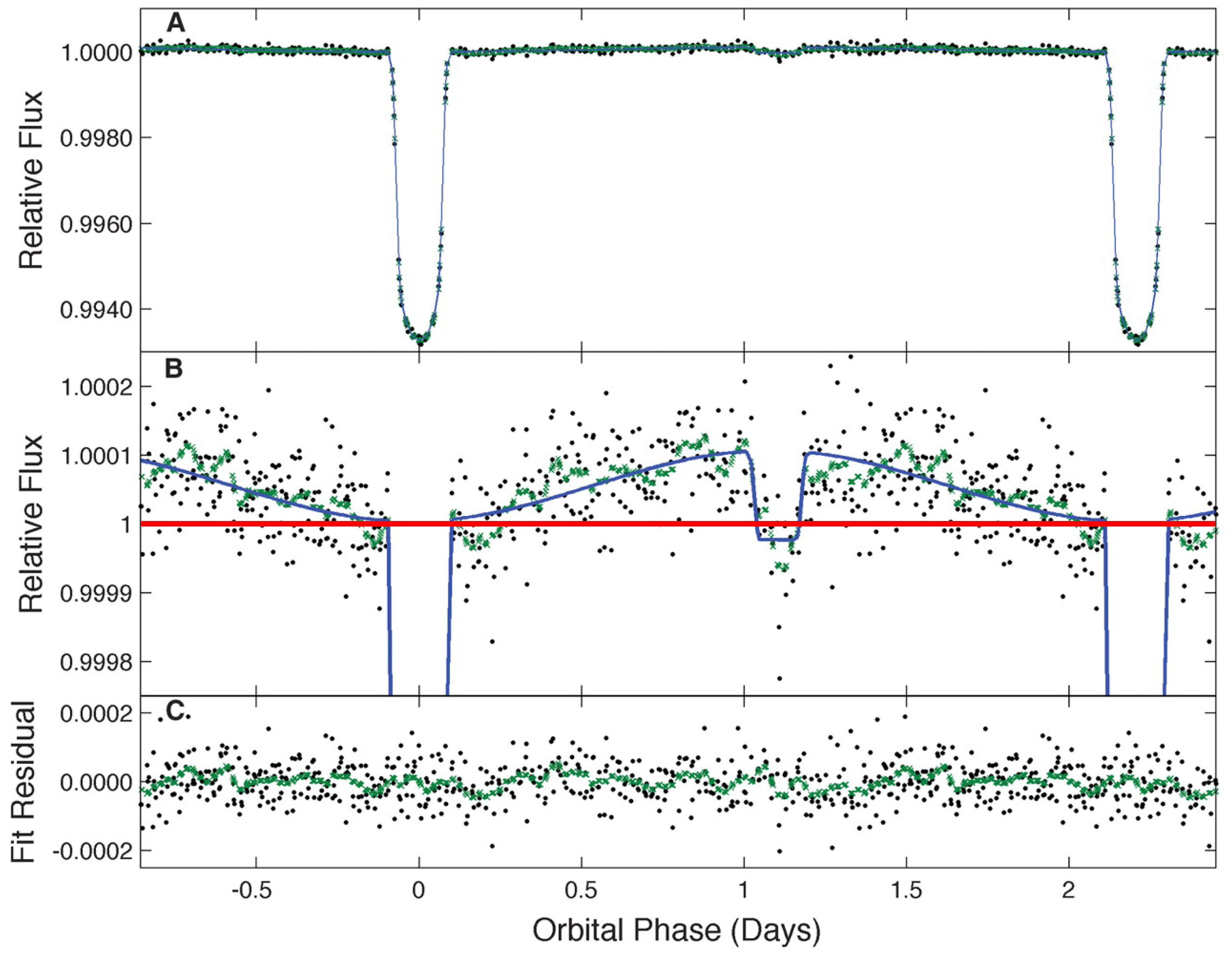
Figure 3 illustrates the recorded data and light curve fit from the exoplanet HAT-P-7b [26]. The primary and secondary eclipses are clearly seen at orbital phase zero days and 1.1 days, respectively. In Figure 3B, planetary flux variations, such as reflected light, are evident in the sinusoidally-varying flux and in the presence of the secondary eclipse as the planet passes behind the host star. The fact that the flux during the secondary eclipse dips below the baseline (red line) indicates that the planet is also emitting a great deal of thermal radiation, which is hidden as the planet passes behind the host star.
4.1. Transits and Eclipses
The most prominent photometric effect is known as the transit or primary transit, which occurs when the planet passes in front of the host star blocking a fraction of the starlight [27]. The primary transit of the exoplanet HAT-P-7b can be seen in Figure 3 at an orbital phase of zero days and again at 2.2 days, which is its orbital period. The bottoms of the primary transits are typically rounded because the light emitted by the star is not uniform across the stellar disk, but is darker near the limbs as one is looking through the cooler upper regions of the photosphere [28]. This effect, known as limb darkening, is illustrated by the coloration of the stars on the left side of Figure 4A,B. The transit depth is proportional to the ratio of cross-sectional areas of the planet and star:
where is the radius of the planet and is the radius of the star.
Transits are relatively rare since the planet must pass between the stellar disk and the observer. Borucki and Summers found the probability that a distant observer could witness an exoplanetary transit to be [29]. This expression was found by considering the solid angle subtended by the exoplanet’s shadow in a circular orbit. Here, we consider eccentric orbits with eccentricity e, and more-or-less follow the derivation by Barnes [30], taking care to rigorously treat the probability distribution associated with the true anomaly, the argument of the periastron and the inclination.
To find the probability of a transit, we first consider circular orbits and work out the prior probability of observing a planet at a given angular position defined by the true anomaly and the inclination, . It is expected that there is no preferred orientation for the inclination of a planet’s orbital plane. Moreover, for a circular orbit, the planet orbits at a constant speed so that the prior probability of the true anomaly is also constant. As a result, the joint prior probability is constant, , where it should be noted that in our expressions for the probability, , we adopt the convention of Jaynes [31] and Sivia and Skilling [19] in which all probabilities are written as being conditional on all of the prior information I about the problem:
so that:
In the case of eccentric orbits, one must also consider the argument of the periastron since:
and the speed of the planet changes as it orbits so that the probability density of finding the planet at a true anomaly of varies with in an elliptical orbit: where .
Consider a change in the viewing angle by , so that and . It is then clear that:
Moreover, since:
and since is periodic, the two integrals over a single period:
and:
are equal so that:
for arbitrary angle . This implies that is constant so that (3) is generally true with:
for both circular and elliptical orbits.
The planet will be observed as transiting only for inclinations between where:
and r is the star-planet distance. Therefore, the probability of a transit:
which is:
Now, using the fact that the star-planet distance r varies as a function of the true anomaly as described in (1), the equation above becomes:
so that in the case of an eccentric orbit, the probability of observing the transit of a planet for which the eccentricity is:
whereas for a circular orbit, or an orbit for which the eccentricity is zero, , the transit probability is:
One can now compute the probability that a distant observer would view a planet in a circular orbit as transiting its host star. Table 1 lists these probabilities for several planets in our solar system for which the Sun has a radius of AU. According to (12), these probabilities fall off as , indicating that the transit method of exoplanet detection is heavily biased toward the detection of closely-orbiting exoplanets.
The probability of an alien civilization being able to observe Earth transiting the Sun (within the Earth transit zone (ETZ)) is only 0.46%. Since the average stellar density in the galactic neighborhood surrounding the Sun is approximately 0.004 stars per cubic light year [32], there are about 17,000 stars within 100 LY of the Sun. Of these 17,000 stars, only about 78 of them are positioned so that Earth could be observed transiting the Sun. A recent study utilized the Hipparcus database to identify 37 K and 45 G dwarf stars in the ETZ within 1000 parsecs (≈3261 LY) [33].
The secondary eclipse is similar to the transit. It occurs when the planet passes behind the host star so that the planetary flux, which is composed of both reflected light and thermal emissions, is blocked. The magnitude of the secondary eclipse is dependent on the magnitude of the planetary flux, which, for a relatively cool planet, is bounded by the maximum amount of reflected light (14):
where we are considering a circular orbit of radius a, is the geometric albedo, is the radius of the planet, is the radius of the host star and is the stellar flux. Since typically , secondary eclipses are not always detectable in the recorded data. EXONEST models secondary eclipses using the methodology developed by Mandel and Agol [28] applied to a uniform source. An example of a secondary eclipse can be seen in Figure 3 at the orbital phase of 1.1 days.
4.2. Reflected Light
Planets reflect light both from cloud tops and from solid or liquid surfaces, and the degree to which they reflect light is quantified by their albedo [15,16,34,35,36]. EXONEST employs the simplest model for reflected light in which the planet is assumed to be diffusely isotropically reflecting, so that the brightness does not depend on the angle of observation. In addition, it is assumed that the planet is situated sufficiently distant from the host star that the starlight impinges on the planet in parallel rays so that half of the planet is in daylight and the other half of the planet is in night.
Given these assumptions, the stellar flux reflected by the planet can be written as [37,38]:
where is the radius of the planet, is the geometric albedo and is the time-varying orbital phase angle. This result appears to work well for many exoplanets.
New Efforts to Properly Model Reflected Light
However, it is known that a significant number of planets (mainly hot Jupiters) closely orbit giant stars so that the assumption that the starlight impinges on the planet in the form of parallel rays is false. Instead, the planet can be divided into three zones. The first zone is that of full daylight where the entire apparent disk of the star can be seen from the surface. The second zone is a penumbral zone where only a portion of the star is visible as it appears to be setting or rising. The third zone is the night zone where the star is not visible. There are a number of cases in which the penumbral zone extends well into what would normally be the night zone. For example, as much as 70% of Kepler-91b’s surface is lit by starlight. This situation is illustrated in Figure 4B. This has significant implications for the primary transit since a fraction of the backside of the planet may be partially illuminated in the penumbral zone, thus compensating somewhat for the reduced starlight due to the transit. As a result, unless the illumination geometry is properly modeled, primary transit depths will be less extensive resulting in an under-estimation of the planetary radius or an over-estimation of the nightside thermal flux followed by an over-estimation of nightside temperatures.
We are currently working to develop reflected light models for EXONEST that can accommodate the case in which planets are illuminated by parallel rays and the case in which planets are illuminated while closely-orbiting giant stars [38,39,40]. The fractional surface areas in the fully-illuminated zone, partially-illuminated penumbral zone and night zone are given by [38]:
Since these surface areas depend on the star-planet separation distance r, eccentric orbits will require the use of the more general reflectance model.
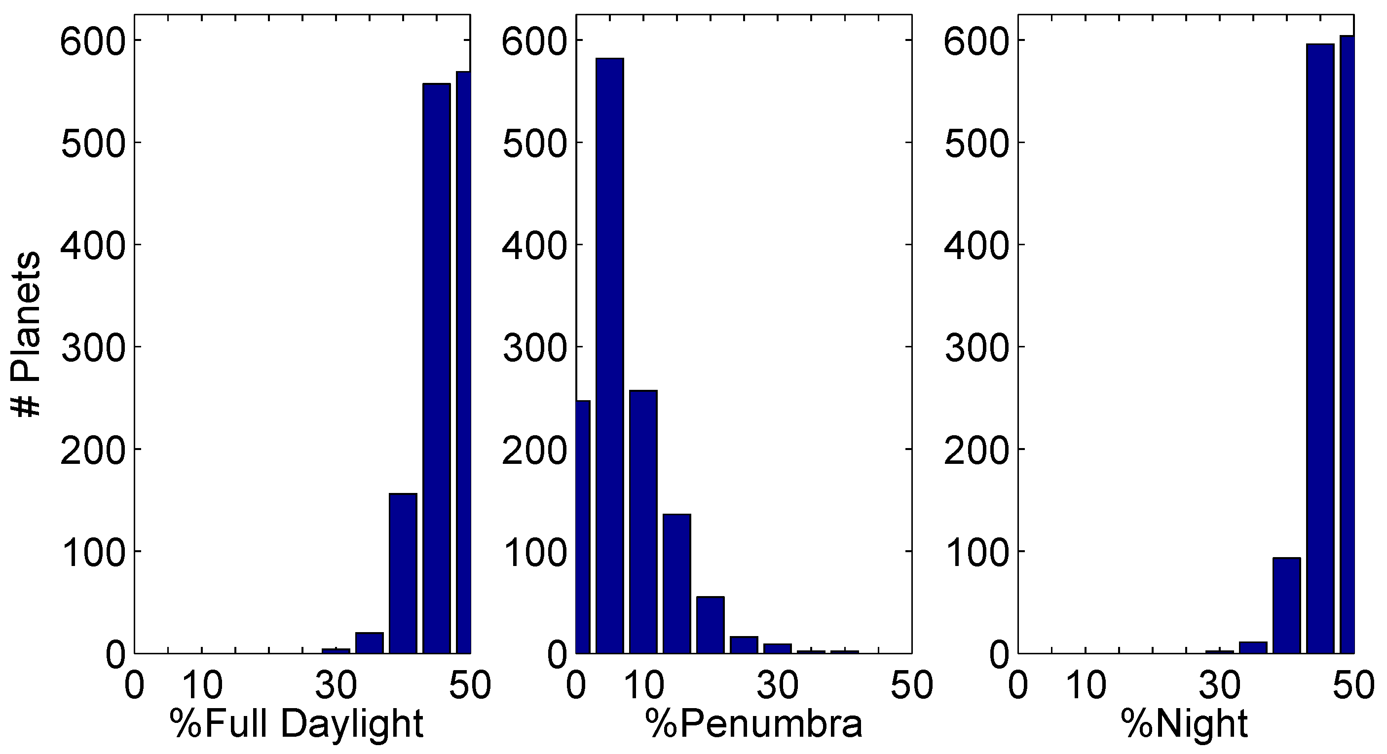
A quick survey of the exoplanet archive [2] reveals 1306 exoplanets for which the radius of the star, , the radius of the planet, , and the semi-major axis, a, are reported. Figure 5 illustrates histograms for these 1306 exoplanets revealing the percent of the surface area that is in full daylight, in a penumbral zone and in completely dark night. It is most common for planets to have a 5% penumbral zone, and more than one quarter of the planets have penumbral zones that are larger than 5%. There are nine planets for which the penumbral zone covers about 30% of the planet’s surface and two planets for which the penumbral zone covers 40% of the planet’s surface! Of these 1306 exoplanets, 39 of them have more than 60% of their surface illuminated (dayside zone plus penumbral zone) by their host star. Another survey of the 1073 confirmed Kepler exoplanets that have orbital periods shorter than 10 days indicates that 88 of those planets (about 8% of them) have more than 60% of their surface illuminated (dayside zone plus penumbral zone) by their host star. The significance of this effect in the context of the reflected light and the analysis of Kepler data will be explored in a future paper.
We believe that improperly modeling stellar illumination was a problem in our earlier study involving a proposed Trojan partner to the planet Kepler-91b. In that analysis, the Bayesian evidence weighed heavily in favor of a Trojan partner, but the modeled planetary temperatures were unphysically high, which led us to discount the possibility of a Trojan partner [41]. The star Kepler-91 is an asymptotic giant branch star with a radius of approximately (where is the solar radius), and the semi-major axis of the hot Jupiter Kepler-91b is AU [42]. The planet Kepler-91b has a radius of , where represents Jupiter’s radius [42]. By Equations (15)–(17), this implies that of Kepler-91b is in full daylight, is in partial penumbral light and is in full darkness, so that approximately of the planet is illuminated at any point in time (as is illustrated in Figure 4B). By not properly accounting for this illumination, the modeled thermal emissions would be forced to compensate with increased day-side and night-side temperatures possibly explaining the unphysically high temperatures obtained in the analysis [41], which led to the Trojan hypothesis being discounted. This is supported by the fact that other studies of this system have led to unphysically high temperatures. For example, a study of KOI-2133b (Kepler-91b) by Esteves et al. [43] found that the nightside temperature was K, which was greater than the expected equilibrium temperature of 1570 K, leading them to hypothesize that Kepler-91b, which was later re-confirmed as a planet [44], was self-luminous.
4.3. Thermal Emissions
The modeling of thermal emissions is similar to that of reflected light. Current models assume that there is a day-side and a night-side and that these two sides are characterized by two effective temperatures and , respectively.
The planet is assumed to radiate as a thermal blackbody so that the detected thermal flux is given by [45]:
where T is the effective temperature of the radiating region, represents the spectral radiance of a blackbody at temperature T:
h is Planck’s constant, is Boltzmann’s constant, and is the Kepler response as a function of wavelength [46].
The relative day-side and night-side fluxes are given by:
with a total relative flux of:
The similarity of the thermal emission phase curve to the reflected light phase curve means that for a circular orbit, the models are degenerate so that it is not possible, using single-bandpass photometry, to distinguish thermal emission from reflected light. Only for significantly eccentric orbits, with , in which the planet-star distance changes, thus affecting reflected light, can thermal flux be modeled independently of reflected light [15], assuming that the temperatures on the planet are relatively constant. Observations in multiple bandpasses, such as combining data from both Kepler and TESS, will enable thermal emissions to be distinguished from reflected light [5]. Just as in the case of reflected light, a closely-orbiting planet will have three zones: a dayside zone, a penumbral zone and a nightside zone. While one could model each zone with a separate average temperature, previous studies have found that the contribution of the penumbral zone to thermal emissions is negligible [47,48].
4.4. New Efforts to Model Refracted and Forward Scattered Light
The situation is significantly more complicated for a planet or moon that possesses an atmosphere. As the planet approaches the primary transit, it becomes more and more backlit. In addition to reflected light from atmospheric clouds or the surface, one detects light that is both forward scattered by the atmosphere and refracted through the atmosphere [49,50,51,52,53]. This effect is illustrated in Figure 6 where in Panel (A), we see an image taken by the Cassini probe of Saturn’s moons Rhea (upper left), Titan (center right) and Mimas (lower center). Both Rhea and Mimas are airless worlds, and one sees only reflected light from their surfaces. Titan, on the other hand, is a large moon with a substantial nitrogen and methane atmosphere. Here, one sees not only reflected light from the cloud tops, but also refracted light through the atmosphere, which makes the illuminated arc much brighter and more extensive than on the other two moons [54].
The increase in photometric flux due to refraction is on the order of [49]:
where H is the scale height of the planetary atmosphere, which is given by:
where is Boltzmann’s constant, T is the average atmospheric temperature, is the mean molecular weight of the atmospheric constituents and g is the gravitational acceleration at the surface of the planet [49]. Typically, , so that by (23), the refractive effects are much smaller than the primary transit depth:
For example, in the case of the Earth ( K, m s, g mol), the characteristic atmospheric height is estimated to be m, which is reasonable considering that the troposphere has an average height of m. As a result, the photometric flux of light refracting through Earth’s atmosphere at the point of occultation is about times, or three orders of magnitude, smaller than than the primary transit depth.
In the event that the photometric effects of refracted light can be detected, this would provide information about the nature of the exoplanetary atmosphere.
4.5. New Efforts to Model Atmospheric Effects
Atmospheric effects can play a significant role in photometry. For example, atmospheric clouds can shift a planet’s highly reflective bright spot away from the substellar point. Similarly, atmospheric superrotation can shift a planet’s thermally bright hotspot away from the substellar point. Such effects, which can be modeled as an angular shift in the reflectance or thermal phase curves, can reveal a great deal about the exoplanetary atmosphere [7,42,55,56]. More exotic effects are possible. For example, it is thought that supersonic flow and shocks can develop on the dayside of irradiated hot Jupiters upstream of the substellar point and that these shocks will affect the position of the peak of the thermal phase curve [57]. Heavily-irradiated hot Jupiters are expected to have an electrically-conductive atmosphere due to ionization. As a result, exoplanetary magnetic fields are expected to affect atmospheric flow [58] and in some cases, magnetically-dragged winds are expected to reduce the longitudinal offset of the thermal hotspot [58,59,60].
Other deviations in the reflectance and thermal phase curves may reveal more about planetary atmospheres, such as inhomogeneous cloud cover across the planet’s surface [61,62], atmospheric variability [63], evolving weather patterns [64,65,66], diurnal atmospheric effects [67] or seasonal atmospheric effects [68].
4.6. Doppler Boosting/Beaming
The gravitational influence of a planet causes both the star and the planet(s) to orbit a common center of mass. As a result, stars with planets tend to wobble. This is the basis of the radial velocity technique in which the radial velocity of the star is carefully measured using spectroscopy and knowledge about the Doppler shift to detect the presence of planets. While the radial velocity technique relies on spectroscopy, there is a photometric component that arises due to relativistic considerations related to stellar aberration in which an object that radiates light uniformly at rest will, in motion, tend to radiate more light in the direction of motion and less light opposite that direction [69]. This effect is called Doppler boosting or Doppler beaming.
The effect can be derived using special relativity resulting in the following formula for the boosted flux [15,16,69]:
where , and where c is the speed of light and is the stellar flux in the reference frame of the star. Since the motion of the star will involve velocities no more than 100–1000 m/s (), it is perhaps surprising that this relativistic effect could be detectable. However, the fact that the star is approximately -times brighter than the reflected light from a planet means that this effect can be on the order of that of reflected light. Given these speeds, a non-relativistic approximation is reasonable:
where represents the radial component of the stellar velocity as viewed from Earth scaled by the speed of light so that:
where is the radial velocity of the planet from the perspective of Earth:
in which is the true anomaly as a function of time, is the argument of the periastron, e is the eccentricity (see Figure 1) and K is the radial velocity semi-amplitude [16] given by:
in which G is Newton’s gravitational constant, T is the period of the planet, is the mass of the planet, i is the inclination of the orbital plane with respect to Earth and is the mass of the star. Note that when the inclination of the orbital plane is zero, , the orbit is face on (in the projected plane of the sky), and both the radial velocity semi-amplitude and the radial velocity are zero, resulting in no Doppler effect. Furthermore, as the planet orbits the star, the true anomaly , which is an angle, advances. There will be two times per orbital period at which the trigonometric factor goes to zero, resulting in zero radial velocity and therefore zero Doppler effect. This is most easily seen by considering a circular orbit for which the eccentricity is zero, , and the argument of the periastron is zero, . In the case of this circular orbit, the radial velocity is zero when the true anomaly is and , which occurs when the planet is moving in the projected plane of the sky. Since the Doppler boosting effect involves both the mass of the planet and the inclination angle of the orbital plane, this phenomenon facilitates the estimation of these two quantities.
4.7. Tidal Forces and Ellipsoidal Variations
Tidal interactions between a massive object and a star create distortions on the star (see Figure 7), which are potentially observable by the Kepler Space Telescope. Known as ellipsoidal variations, this photometric effect appears with two maxima per orbit, each occurring when the largest cross-sectional area of stellar surface is observed. Bayesian model testing provides a rigorous framework to compare the various representations of ellipsoidal variations. A preferred representation of ellipsoidal variations will become increasingly important for exoplanet classification with higher precision photometry.
4.7.1. Trigonometric Models
The BEaming, Ellipsoidal and Reflection (BEER) model, which was developed by Faigler and Mazeh [70], models the ellipsoidal variations as being proportional to the cosine of twice the phase angle:
in which on the left-hand side, the flux due to the ellipsoidal variations is normalized by the stellar flux , is the planet’s mass, is the star’s mass, is the star’s radius, a is the star-planet distance, i is the inclination of the orbital plane and is the orbital phase [0, ]. The BEER model allows for positive and negative values for the amount of ellipsoidal variation observed. The effects of linear gravity-darkening and limb-darkening, , are modeled by [71]:
in which the linear limb-darkening and gravity-darkening coefficients are represented by u and g, respectively. Estimates of the coefficients u and g are provided by modeling metallicity and effective stellar temperature [72,73].
The Kane and Gelino model hypothesizes ellipsoidal variations to be proportional to the projected separation distance between the star and planet [74], which, when substituted for the orbital phase, become:
However, this model suffers from a discontinuity in the first derivative, which is not seen in simulations of ellipsoidal variations using gravitational isopotentials.
A modified form, labeled Kane and Gelino (Mod), was introduced by Placek et al. [15], which removes the discontinuity by setting the effect proportional to the square of the projected separation distance:
Unlike the BEER model, which produces negative values, the two Kane and Gelino models have a minimum value of zero.
4.7.2. Direct Modeling: EVIL-MC
The Ellipsoidal Variations Induced by a Low-Mass Companion (EVIL-MC) model was developed by Jackson et al. [75] to directly model tidal effects on the stellar atmosphere. EVIL-MC was modified for use in EXONEST [76,77] in which a geodesic structure of 640 triangles is used to represent the stellar surface as illustrated in Figure 7. The deviations from sphericity are computed for each point on the surface model. The observed flux, , is computed by summing the blackbody flux within the Kepler bandpass (18) over the observed surface area. The ellipsoidal variation effect is then computed with:
where is the flux from a spherical star and is the flux from the ellipsoidal star. While direct modeling should provide a more accurate representation, EVIL-MC is significantly (≈1000–10,000 times) more computationally expensive than the trigonometric models. The Kane and Gelino (Mod) model provides a computationally fast approximation to EVIL-MC.
4.7.3. Model Testing
We have recently performed model testing on Kepler light curve data using EXONEST [76,77]. EVIL-MC provided the best representation of ellipsoidal variations in the Kepler-13 system followed by the Kane and Gelino (Mod) and BEER models, which had similar evidence values. The values are reported in Table 2. The Kane and Gelino (Mod) model is closest to the EVIL-MC results and has slightly higher evidence over the others suggesting that, given its straight-forward analytic form, the Kane and Gelino (Mod) is the most effective model for this effect.
5. Bayesian Inference Engine
For a given exoplanetary model, the Bayesian inference engine allows us to compute the Bayesian evidence and the model parameter values along with their associated uncertainties. The current implementation allows for a choice of sampling methods: Metropolis–Hastings Markov chain Monte Carlo (MCMC) [23,24] (which does not provide the Bayesian evidence), the original nested sampling algorithm [17,18,19] or the more recent variant called MultiNest [20,21,22]. While the MultiNest algorithm has proven to shorten run times from several days to 10s of hours, it is usually not possible to operate with more than 75 samples, which severely reduces the precision to which the Bayesian evidence and the parameter values can be estimated.
Unfortunately, even by integrating a single period in cases with one exoplanet, the time required to evaluate the log likelihood is too great to allow for a rapid analysis. It may be of benefit to re-parameterize the eccentricity and argument of periapsis as suggested by Ford [78]. In addition, since we have found almost no evidence of phase changes in our analyses to date, it has been suggested (P. Goggans, personal communication) that EXONEST be designed to utilize simulated annealing.
Model testing is a significant part of the EXONEST analysis pathway. By turning on-and-off various photometric models and comparing the Bayesian evidence in each case, one can build a case that a candidate exoplanet is a real planet and not a false positive [15,79].
Priors and Likelihoods
EXONEST allows priors on the parameter values to be specified. However, since we are still learning a great deal about exoplanets, the assignment of an informative prior based on known exoplanets is potentially detrimental as it may bias against the discovery of new phenomena. For this reason, uniform or non-informative priors are most often used.
Likelihoods can also be specified for EXONEST. While Gaussian likelihoods are typically employed, there have been situations involving asymptotic giant branch stars in which likelihoods that accommodate correlated noise (red noise) are necessary [41], prompting us to implement Sivia’s nearest-neighbor approach [19]:
where N is the number of data points, is the noise variance, is the correlation strength, which is a parameter to be estimated, and Q depends on the sum of the square of the residuals by:
The quantity is the sum of the first and the last squared residuals, and is the sum of the nearest neighbor squared residuals:
As usual, the residuals are given by the difference between the modeled relative flux and the observed relative flux. In practice, one divides the observed flux by the average of the observed flux to obtain the observed relative flux. The residuals are typically given by:
where is the observed or measured photometric flux at time and is the sum of the modeled relative photometric fluxes at time . Unfortunately, this practice is not ideal since it is not generally true that since the photometric effects (transits, etc.) do not all integrate to zero. In principle, one could subtract the flux during the secondary eclipse, since ellipsoidal variations will be minimal and there will be no planetary effects. However, it would be better to model the stellar flux and to marginalize over it.
It is a straightforward problem to incorporate additional data, such as radial velocity measurements, by adding terms to the log likelihood. This has been done in our study of the Kepler-91 system [41].
6. Application: Kepler-76b
Kepler-76b is a transiting hot-Jupiter with a radius of approximately that orbits a star with an orbital period of days [80]. This planet is known to exhibit reflection/thermal emission, Doppler boosting, as well as ellipsoidal variations [42,80,81]. This section outlines EXONEST’s model selection capabilities with fits of four different forward models that each account for different combinations of photometric effects. The simplest model includes only the reflection component (R), which in the case of a circular orbit subsumes thermal emission. The second model includes reflection and ellipsoidal variations (RE). The third model accounts for reflection, ellipsoidal variations and Doppler beaming (REB). Finally, the last model accounts for each of the three effects in the REB model in addition to an angular shift in the phase curve (reflection component), which is indicative of atmospheric superrotation (REB-SR). The data, which were obtained from the Mikulski Archive for Space Telescopes (MAST) managed by the Space Telescope Science Institute (STScI), consists of all available quarters of long-cadence Kepler Space Telescope data for Kepler-76b. The data were preprocessed to remove the primary transit so that only the overall phase curve and the secondary eclipse were fit by the EXONEST models. Note that even without considering the primary transit, excellent parameter estimates were obtained.
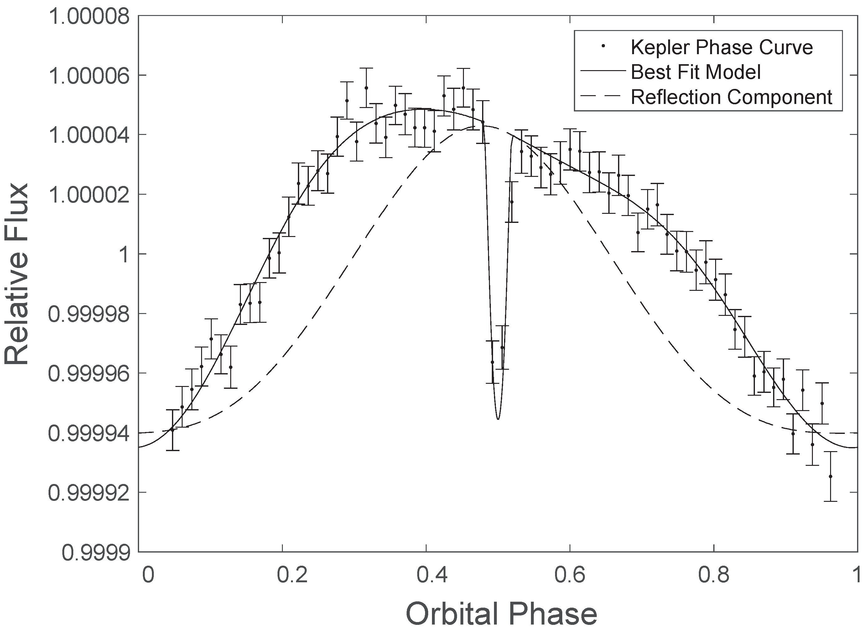
The results of the model testing are listed in Table 3. In this example, the most complex model (REB-SR), illustrated in Figure 8, was favored by both the Bayesian evidence () and the maximum log-likelihood () to explain the data. We can thus claim the detection of a shift in the phase curve by 8.53 0.12 degrees westward of the sub-stellar point, which is most likely caused by atmospheric superrotation. This result is consistent with previous studies of Kepler-76b, which yielded estimated westward shifts of 10.3 2.0 [80] and 8.28 1.22 [42]. The parameter estimates for the REB-SR model are listed in Table 4. Note that these estimates are comparable to those reported [80] when Kepler-76b was discovered.
7. Conclusions
EXONEST: The Exoplanetary Explorer is a software package for detecting and characterizing exoplanets from Kepler and CoRoT data. The package models a large number of photometric effects, each of which provides valuable information about the exoplanet and the exoplanetary system. New efforts include developing more precise models of reflected light, refracted light and atmospheric effects, as well as re-coding to transform EXONEST into a Python-based open source project with the capability to employ third-party plug-and-play models of exoplanet-related photometric effects. In addition, new planetary models are being developed that are relevant to rapidly rotating planets with shapes ranging from that of an oblate ellipsoid to pyriform shapes [82] and synestias [83]. These features are summarized in Table 5.
While it is true that by adding more parameters, one can over-fit the data by increasing the likelihood, for this reason, EXONEST employs Bayesian model testing, which enables one to evaluate the significance of each photometric effect. The model testing capabilities of EXONEST were demonstrated on Kepler Space Telescope of Kepler-76. Kepler-76b was demonstrated to exhibit several photometric effects: reflected light, Doppler boosting, ellipsoidal variations and atmospheric superrotation. Parameter estimates were reported that are in agreement with previous studies [42,80,81] using both radial velocity and photometric data. In addition, the model testing capabilities of EXONEST enable one to test photometric models against one another.
Future missions promise instruments of increasing sensitivity and detail with multiple spectral bands. Despite this, photometry will continue to be a valuable resource until detailed direct imaging is possible. In the meantime, we aim to include more relevant photometric effects into EXONEST and to develop the software package to work in conjunction with future multispectral studies.
Acknowledgments
This paper was presented as an invited talk at the 37th International Workshop on Bayesian Inference and Maximum Entropy Methods in Science and Engineering (MaxEnt 2017) in Jarinu SP, Brasil. Knuth would like to thank the organizers, Adriano Polpo and Julio Stern, for both the kind invitation and their generous hospitality. We also wish to thank Jon Jenkins, Doug Caldwell, John Skilling, Paul Goggans, Wesley Henderson, Ariel Caticha, Keith Earle, Oleg Lunin and Matthew Szydagis for interesting discussions and helpful advice, questions and comments. We would also like to thank the two anonymous reviewers whose comments served to improve the quality of this manuscript.
Author Contributions
K.H.K. and B.P. conceived of EXONEST. K.H.K. advised the research and work performed by B.P., J.L.C., B.D., A.D.G., and B.C., and wrote the greater part of the manuscript. B.P. developed, coded, tested, and utilized EXONEST as a major component of his Ph.D. research. B.P. performed the analysis of Kepler-76b and wrote the corresponding section of the manuscript. D.A. contributed to the development of EXONEST and the inclusion of several photometric effects. As the focus of her Ph.D. research, J.L.C. has led the effort to more accurately model reflected light, and she contributed to the writing of the section on reflected light. As the focus of his M.S. thesis, B.D. implemented the three-body orbital code. As the focus of his M.S. thesis, A.D.G. coded and tested the efficacy of stellar ellipsoidal variation models, and wrote the corresponding section on ellipsoidal variations. B.C. assisted J.L.C. in the modeling of reflected light, and as the focus of his Ph.D. research, he has worked to characterize planetary shapes and their transit signatures.
Conflicts of Interest
The authors declare no conflict of interest.
References
- NASA. NASA Strategic Plan 2014; The National Aeronautics and Space Administration: Washington, DC, USA, 2014.
- Caltech. NASA Exoplanet Archive. Available online: https://exoplanetarchive.ipac.caltech.edu/ (accessed on 1 August 2017).
- Borucki, W.J.; Koch, D.; Basri, G.; Batalha, N.; Brown, T.; Caldwell, D.; Caldwell, J.; Christensen-Dalsgaard, J.; Cochran, W.D.; DeVore, E.; et al. Kepler Planet-Detection Mission: Introduction and First Results. Science 2010, 327, 977–980. [Google Scholar] [CrossRef] [PubMed]
- Ricker, G.R.; Latham, D.W.; Vanderspek, R.K.; Ennico, K.A.; Bakos, G.; Brown, T.M.; Burgasser, A.J.; Charbonneau, D.; Clampin, M.; Deming, L.D.; et al. Transiting Exoplanet Survey Satellite (TESS). Bull. Am. Astron. Soc. 2010, 42, 459. [Google Scholar]
- Placek, B.; Knuth, K.H.; Angerhausen, D. Combining photometry from Kepler and TESS to improve short-period exoplanet characterization. Publ. Astron. Soc. Pac. 2016, 128, 074503. [Google Scholar] [CrossRef]
- Beichman, C.; Benneke, B.; Knutson, H.; Smith, R.; Lagage, P.O.; Dressing, C.; Latham, D.; Lunine, J.; Birkmann, S.; Ferruit, P.; et al. Observations of transiting exoplanets with the James Webb Space Telescope (JWST). Publ. Astron. Soc. Pac. 2014, 126, 1134. [Google Scholar] [CrossRef]
- Placek, B.; Angerhausen, D.; Knuth, K.H. Optimizing Observing Strategies for Exoplanet Secondary Eclipses and Phase Curves. Astrophys. J. 2017, in press. [Google Scholar]
- ESA. Science and Technology: CHEOPS. Available online: http://sci.esa.int/cheops/ (accessed on 30 September 2016).
- CHEOPS Science Team—University of Bern. CHEOPS Mission Homepage. Available online: http://cheops.unibe.ch/ (accessed on 28 March 2017).
- Broeg, C.; Fortier, A.; Ehrenreich, D.; Alibert, Y.; Baumjohann, W.; Benz, W.; Deleuil, M.; Gillon, M.; Ivanov, A.; Liseau, R.; et al. CHEOPS A Transit Photometry Mission for ESA’s Small Mission Programme. EPJ Web Conf. 2013, 47. [Google Scholar] [CrossRef]
- ESA. Science and Technology: PLATO. Available online: http://sci.esa.int/plato/ (accessed on 30 September 2016).
- ESA Study Team; PLATO Science Study Team. PLATO Science Study Team. PLATO Science Requirements Document. In ESA Public Documents; ESA Study Team; PLATO Science Study Team, 2010. [Google Scholar]
- Hippke, M.; Angerhausen, D. Photometry’s Bright Future: Detecting Solar System Analogs with Future Space Telescopes. Astrophys. J. 2015, 810, 29. [Google Scholar] [CrossRef]
- NASA. Wide Field Infrared Survey Telescope. Available online: https://wfirst.gsfc.nasa.gov/index.html (accessed on 29 October 2016).
- Placek, B.; Knuth, K.H.; Angerhausen, D. EXONEST: Bayesian model selection applied to the detection and characterization of exoplanets via photometric variations. Astrophys. J. 2014, 795, 112. [Google Scholar] [CrossRef]
- Placek, B. Bayesian Detection and Characterization of Extra-Solar Planets via Photometric Variations. Ph.D. Thesis, University at Albany (SUNY), Albany, NY, USA, 2014. [Google Scholar]
- Skilling, J. Nested sampling. In Bayesian Inference and Maximum Entropy Methods in Science and Engineering, Garching, Germany 2004; Fischer, R., Dose, V., Preuss, R., von Toussaint, U., Eds.; American Institute of Physics (AIP): New York, NY, USA, 2004; pp. 395–405. [Google Scholar]
- Skilling, J. Nested sampling for general Bayesian computation. Bayesian Anal. 2006, 1, 833–859. [Google Scholar] [CrossRef]
- Sivia, D.S.; Skilling, J. Data Analysis. A Bayesian Tutorial, 2nd ed.; Oxford University Press: Oxford, UK, 2006. [Google Scholar]
- Feroz, F.; Hobson, M.P.; Bridges, M. MultiNest: An efficient and robust Bayesian inference tool for cosmology and particle physics. Mon. Not. R. Astron. Soc. 2009, 398, 1601–1614. [Google Scholar] [CrossRef]
- Feroz, F.; Balan, S.T.; Hobson, M.P. Detecting extrasolar planets from stellar radial velocities using Bayesian evidence. Mon. Not. R. Astron. Soc. 2011, 415, 3462–3472. [Google Scholar] [CrossRef]
- Feroz, F.; Hobson, M.P.; Cameron, E.; Pettitt, A.N. Importance nested sampling and the MultiNest algorithm. arXiv, 2013; arXiv:1306.2144. [Google Scholar]
- Metropolis, N.; Rosenbluth, A.W.; Rosenbluth, M.N.; Teller, A.H.; Teller, E. Equations of state calculations by fast computing machines. J. Chem. Phys. 1953, 21, 1087–1092. [Google Scholar] [CrossRef]
- Hastings, W.K. Monte Carlo Sampling Methods Using Markov Chains and Their Applications. Biometrika 1970, 57, 97–109. [Google Scholar] [CrossRef]
- Brown, R.A. Photometric orbits of extrasolar planets. Astrophys. J. 2009, 702, 1237. [Google Scholar] [CrossRef]
- Borucki, W.J.; Koch, D.; Jenkins, J.; Sasselov, D.; Gilliland, R.; Batalha, N.; Latham, D.W.; Caldwell, D.; Basri, G.; Brown, T.; et al. Kepler’s Optical Phase Curve of the Exoplanet HAT-P-7b. Science 2009, 325, 709. [Google Scholar] [CrossRef] [PubMed]
- Seager, S.; Mallěn-Ornelas, G. A unique solution of planet and star parameters from an extrasolar planet transit light curve. Astrophys. J. 2003, 585, 1038. [Google Scholar] [CrossRef]
- Mandel, K.; Agol, E. Analytic light curves for planetary transit searches. Astrophys. J. Lett. 2002, 580, L171. [Google Scholar] [CrossRef]
- Borucki, W.J.; Summers, A.L. The photometric method of detecting other planetary systems. Icarus 1984, 58, 121–134. [Google Scholar] [CrossRef]
- Barnes, J.W. Effects of Orbital Eccentricity on Extrasolar Planet Transit Detectability and Light Curves. Publ. Astron. Soc. Pac. 2007, 119, 986. [Google Scholar] [CrossRef]
- Jaynes, E.T. Probability Theory: The Logic of Science; Cambridge University Press: Cambridge, UK, 2003. [Google Scholar]
- Gregersen, E. The Milky Way and Beyond: Stars, Nebulae, and Other Galaxies; The Rosen Publishing Group: New York, NY, USA, 2010. [Google Scholar]
- Heller, R.; Pudritz, R.E. The search for extraterrestrial intelligence in Earth’s solar transit zone. Astrobiology 2016, 16, 259–270. [Google Scholar] [CrossRef] [PubMed]
- Jenkins, J.M.; Doyle, L.R. Detecting reflected light from close-in extrasolar giant planets with the Kepler photometer. Astrophys. J. 2003, 595, 429–445. [Google Scholar] [CrossRef]
- Seager, S. Exoplanet Atmospheres: Physical Processes; Princeton University Press: Princeton, NJ, USA, 2010. [Google Scholar]
- Perryman, M. The Exoplanet Handbook; Cambridge University Press: Cambridge, UK, 2011. [Google Scholar]
- Sobolev, V.V. Light Scattering in Planetary Atmospheres; Pergamon Press: Oxford, UK, 1975. [Google Scholar]
- Carter, J. Estimation of Planetary Photometric Emissions for Extremely Close-in Exoplanets. Ph.D. Thesis, University at Albany, Albany, NY, USA, 2017. in progress. [Google Scholar]
- Ḱopal, Z. Photometric Effects of Reflection in Close Binary Systems. Mon. Not. R. Astron. Soc. 1954, 114, 101–117. [Google Scholar] [CrossRef]
- Ḱopal, Z. Close Binary Systems; John Wiley and Sons Inc.: New York, NY, USA, 1959. [Google Scholar]
- Placek, B.; Knuth, K.; Angerhausen, D.; Jenkins, J. Characterization of Kepler-91b and the investigation of a potential Trojan companion using EXONEST. Astrophys. J. 2015, 814, 147. [Google Scholar] [CrossRef]
- Esteves, L.; De Mooij, E.; Jayawardhana, R. Changing phases of alien worlds: Probing atmospheres of Kepler planets with high-precision photometry. Astrophys. J. 2015, 804, 150. [Google Scholar] [CrossRef]
- Esteves, L.J.; De Mooij, E.J.W.; Jayawardhana, R. Optical phase curves of Kepler exoplanets. Astrophys. J. 2013, 772, 51. [Google Scholar] [CrossRef]
- Sliski, D.H.; Kipping, D.M. A high false positive rate for Kepler planetary candidates of giant stars using asterodensity profiling. Astrophys. J. 2014, 788, 148. [Google Scholar] [CrossRef]
- Charbonneau, D.; Allen, L.E.; Megeath, S.T.; Torres, G.; Alonso, R.; Brown, T.M.; Gilliland, R.L.; Latham, D.W.; Mandushev, G.; O’Donovan, F.T.; et al. Detection of thermal emission from an extrasolar planet. Astrophys. J. 2005, 626, 523. [Google Scholar] [CrossRef]
- Van Cleve, J.E.; Caldwell, D.A. Kepler Instrument Handbook; NASA/Ames Research Center: Moffett Field, CA, USA, 2009.
- Léger, A.; Grasset, O.; Fegley, B.; Codron, F.; Albarede, A.F.; Barge, P.; Barnes, R.; Cance, P.; Carpy, S.; Catalano, F.; et al. The extreme physical properties of the CoRoT-7b super-Earth. Icarus 2011, 213, 1–11. [Google Scholar] [CrossRef] [Green Version]
- Maurin, A.S.; Selsis, F.; Hersant, F.; Belu, A. Thermal phase curves of nontransiting terrestrial exoplanets-II. Characterizing airless planets. Astron. Astrophys. 2012, 538, A95. [Google Scholar] [CrossRef]
- Sidis, O. Transits of transparent planets Atmospheric lensing effects. Astrophys. J. 2010, 720, 904. [Google Scholar] [CrossRef]
- Misra, A. The Effects of Refraction and Forward Scattering on Exoplanet Transit Transmission Spectroscopy. Ph.D. Thesis, University of Washington, Seattle, WA, USA, 2015. [Google Scholar]
- Misra, A.; Meadows, V.; Crisp, D. The effects of refraction on transit transmission spectroscopy: Application to Earth-like exoplanets. Astrophys. J. 2014, 792, 61. [Google Scholar] [CrossRef]
- Bétrémieux, Y.; Kaltenegger, L. Refraction in planetary atmospheres: Improved analytical expressions and comparison with a new ray-tracing algorithm. Mon. Not. R. Astron. Soc. 2015, 451, 1268–1283. [Google Scholar] [CrossRef]
- Muñoz, A.G.; Cabrera, J. Exoplanet phase curves at large phase angles. Diagnostics for extended hazy atmospheres. Mon. Not. R. Astron. Soc. 2017, in press. [Google Scholar]
- Muñoz, A.G.; Lavvas, P.; West, R.A. Titan brighter at twilight than in daylight. Nat. Astron. 2017, 1. [Google Scholar] [CrossRef]
- Showman, A.P.; Polvani, L.M. Equatorial superrotation on tidally locked exoplanets. Astrophys. J. 2011, 738, 71. [Google Scholar] [CrossRef]
- Faigler, S.; Mazeh, T. BEER Analysis of Kepler and CoRoT Lightcurves. II. Evidence for Superrotation in the Phase Curves of Three Kepler Hot Jupiters. Astrophys. J. 2015, 800, 73. [Google Scholar] [CrossRef]
- Heng, K. On the existence of shocks in irradiated exoplanetary atmospheres. Astrophys. J. Lett. 2012, 761, L1. [Google Scholar] [CrossRef]
- Batygin, K.; Stanley, S.; Stevenson, D.J. Magnetically Controlled Circulation on Hot Extrasolar Planets. Astrophys. J. 2013, 776, 53. [Google Scholar] [CrossRef]
- Menou, K. Magnetic scaling laws for the atmospheres of hot giant exoplanets. Astrophys. J. 2012, 745, 138. [Google Scholar] [CrossRef]
- Rauscher, E.; Menou, K. Three-dimensional Atmospheric Circulation Models of HD 189733b and HD 209458b with Consistent Magnetic Drag and Ohmic Dissipation. Astrophys. J. 2013, 764, 103. [Google Scholar] [CrossRef]
- Demory, B.O.; De Wit, J.; Lewis, N.; Fortney, J.; Zsom, A.; Seager, S.; Knutson, H.; Heng, K.; Madhusudhan, N.; Gillon, M.; et al. Inference of inhomogeneous clouds in an exoplanet atmosphere. Astrophys. J. Lett. 2013, 776, L25. [Google Scholar] [CrossRef]
- Heng, K.; Demory, B.O. Understanding Trends Associated with Clouds in Irradiated Exoplanets. Astrophys. J. 2013, 777, 100. [Google Scholar] [CrossRef]
- Armstrong, D.J.; de Mooij, E.; Barstow, J.; Osborn, H.P.; Blake, J.; Saniee, N.F. Variability in the atmosphere of the hot giant planet HAT-P-7 b. Nat. Astron. 2016, 1. [Google Scholar] [CrossRef]
- Pallé, E.; Ford, E.B.; Seager, S.; Montañés-Rodríguez, P.; Vazquez, M. Identifying the rotation rate and the presence of dynamic weather on extrasolar Earth-like planets from photometric observations. Astrophys. J. 2008, 676, 1319. [Google Scholar] [CrossRef]
- Artigau, É.; Bouchard, S.; Doyon, R.; Lafrenière, D. Photometric variability of the T2. 5 brown dwarf SIMP J013656. 5+ 093347: Evidence for evolving weather patterns. Astrophys. J. 2009, 701, 1534. [Google Scholar] [CrossRef]
- Gillon, M.; Triaud, A.H.M.J.; Jehin, E.; Delrez, L.; Opitom, C.; Magain, P.; Lendl, M.; Queloz, D. Fast-evolving weather for the coolest of our two new substellar neighbours. Astron. Astrophys. 2013, 555, L5. [Google Scholar] [CrossRef]
- Ford, E.B.; Seager, S.; Turner, E.L. Characterization of extrasolar terrestrial planets from diurnal photometric variability. Nature 2001, 412, 885–887. [Google Scholar] [CrossRef] [PubMed]
- Van Eylen, V.; Nielsen, M.L.; Hinrup, B.; Tingley, B.; Kjeldsen, H. Investigation of systematic effects in Kepler data: Seasonal variations in the light curve of HAT-P-7b. Astrophys. J. Lett. 2013, 774, L19. [Google Scholar] [CrossRef]
- Rybicki, G.B.; Lightman, A.P. Radiative Processes in Astrophysics; John Wiley and Sons: Hoboken, NJ, USA, 2008. [Google Scholar]
- Faigler, S.; Mazeh, T. Photometric Detection of non-transiting Short-Period Low-Mass companions through the beaming, ellipsoidal, and reflection effects in Kepler and CoRoT light curves. Mon. Not. R. Astron. Soc. 2011, 415, 3921–3928. [Google Scholar] [CrossRef]
- Morris, S.L. The Ellipsoidal Variable Stars. Astrophys. J. 1985, 295, 143–152. [Google Scholar] [CrossRef]
- Heyrovský, D. Computing Limb-Darkening Coefficients from Stellar Atmosphere Models. Astrophys. J. 2007, 656, 483–492. [Google Scholar] [CrossRef]
- Sing, D. Stellar Limb-Darkening Coefficients for CoRoT and Kepler. Astron. Astrophys. 2010, 510, A21. [Google Scholar] [CrossRef]
- Kane, S.R.; Gelino, D.M. Distinguishing Between Stellar and Planetary Companions with Phase Monitoring. Mon. Not. R. Astron. Soc. 2012, 424, 779–788. [Google Scholar] [CrossRef]
- Jackson, B.K.; Lewis, N.; Barnes, J.; Deming, L.; Showman, A.; Fortney, J. The EVIL-MC Model for Ellipsoidal Variations of Planet-Hosting Stars and Applications to the HAT-P-7 System. Astrophys. J. 2012, 751, 112. [Google Scholar] [CrossRef]
- Gai, A. Bayesian Model Testing of Models for Ellipsoidal Variation on Stars Due to Hot Jupiters. Master’s Thesis, University at Albany, Albany, NY, USA, 2016. [Google Scholar]
- Gai, A.; Knuth, K.H. Bayesian Model Testing of Ellipsoidal Variations on Stars Due to Hot Jupiters; Anthony Gai (Univeraity at Albany): Albany, NY, USA, 2017; in press. [Google Scholar]
- Ford, E.B. Improving the Efficiency of Markov Chain Monte Carlo for Analyzing the Orbits of Extrasolar Planets. Astrophys. J. 2006, 642, 505. [Google Scholar] [CrossRef]
- Knuth, K.H.; Habeck, M.; Malakar, N.K.; Mubeen, A.M.; Placek, B. Bayesian evidence and model selection. Digit. Signal Process. 2015, 47, 50–67. [Google Scholar] [CrossRef]
- Faigler, S.; Tal-Or, L.; Mazeh, T.; Latham, D.W.; Buchhave, L.A. BEER Analysis of Kepler and CoRoT Light Curves. I. Discovery of Kepler-76b: A Hot Jupiter with Evidence for Superrotation. Astrophys. J. 2013, 771, 26. [Google Scholar] [CrossRef]
- Angerhausen, D.; DeLarme, E.; Morse, J.A. A Comprehensive Study of Kepler Phase Curves and Secondary Eclipses: Temperatures and Albedos of Confirmed Kepler Giant Planets. Publ. Astron. Soc. Pac. 2015, 127, 1113–1130. [Google Scholar] [CrossRef]
- Abraham, R.H.; Shaw, C.D. Dynamics-The Geometry of Behavior: Vol.: 2: Chaotic Behavior; Aerial Press, Incorporated: Santa Cruz, CA, USA, 1983. [Google Scholar]
- Lock, S.J.; Stewart, S.T. The structure of terrestrial bodies: Impact heating, corotation limits, and synestias. J. Geophys. Res. Planets 2017, 122, 950–982. [Google Scholar] [CrossRef]
Figure 1.
An illustration of the structure of the EXONEST software package.
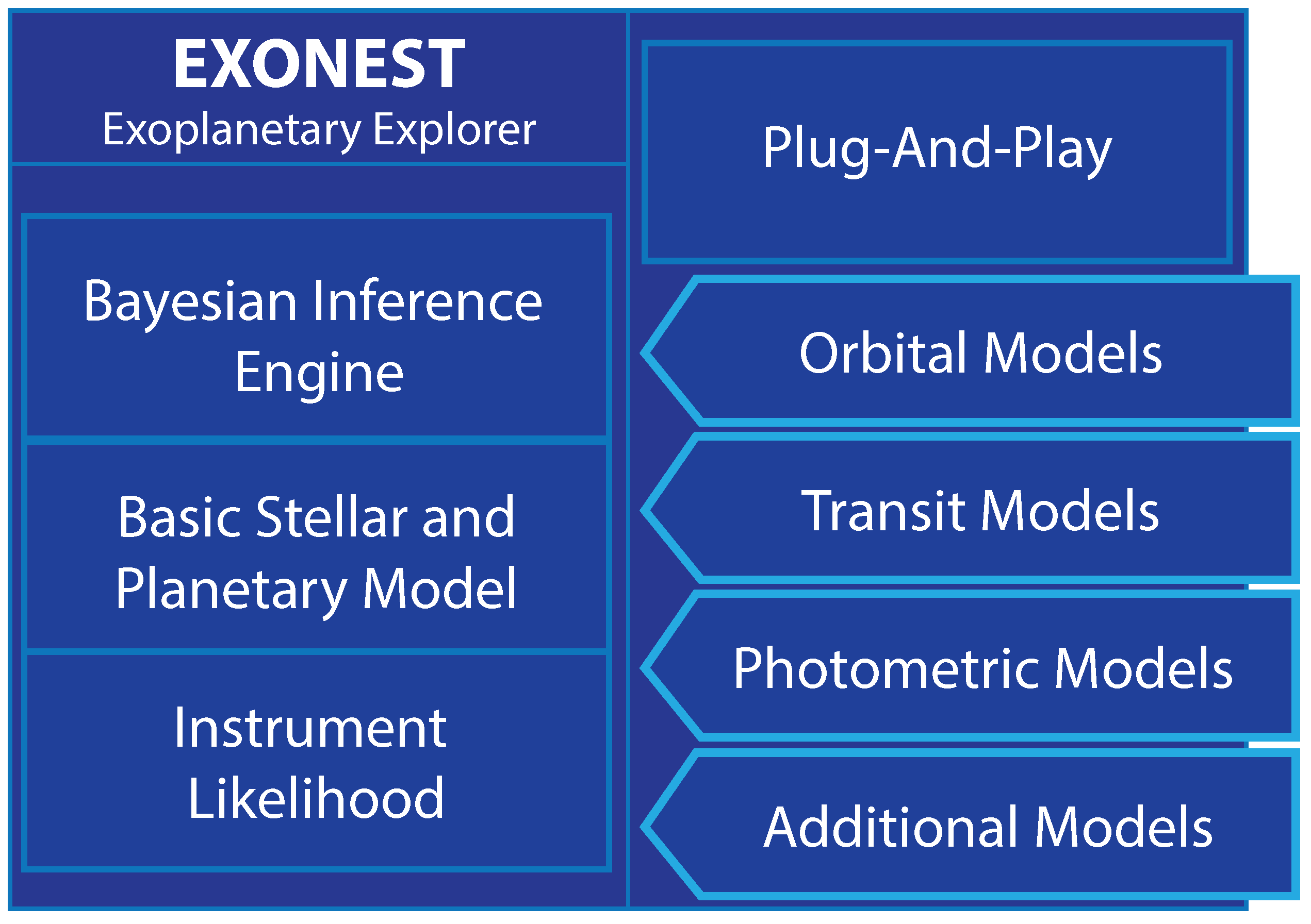
Figure 2.
(A) An illustration of the anatomy of a typical Keplerian orbit. The planet moves on an elliptical orbit with the star located at one focus. The semi-major axis, a, of the ellipse is used to characterize the star-planet distance. The argument of the periastron, , is the angle describing how the periastron (point of closest approach) is rotated with respect to the observer. The true anomaly, , describes the position of the planet along the orbit in the frame of the host star with the origin at the periastron. (B) The angle indicates the orbital phase, which is defined as the angle between the planet-star vector and the planet-Earth vector.
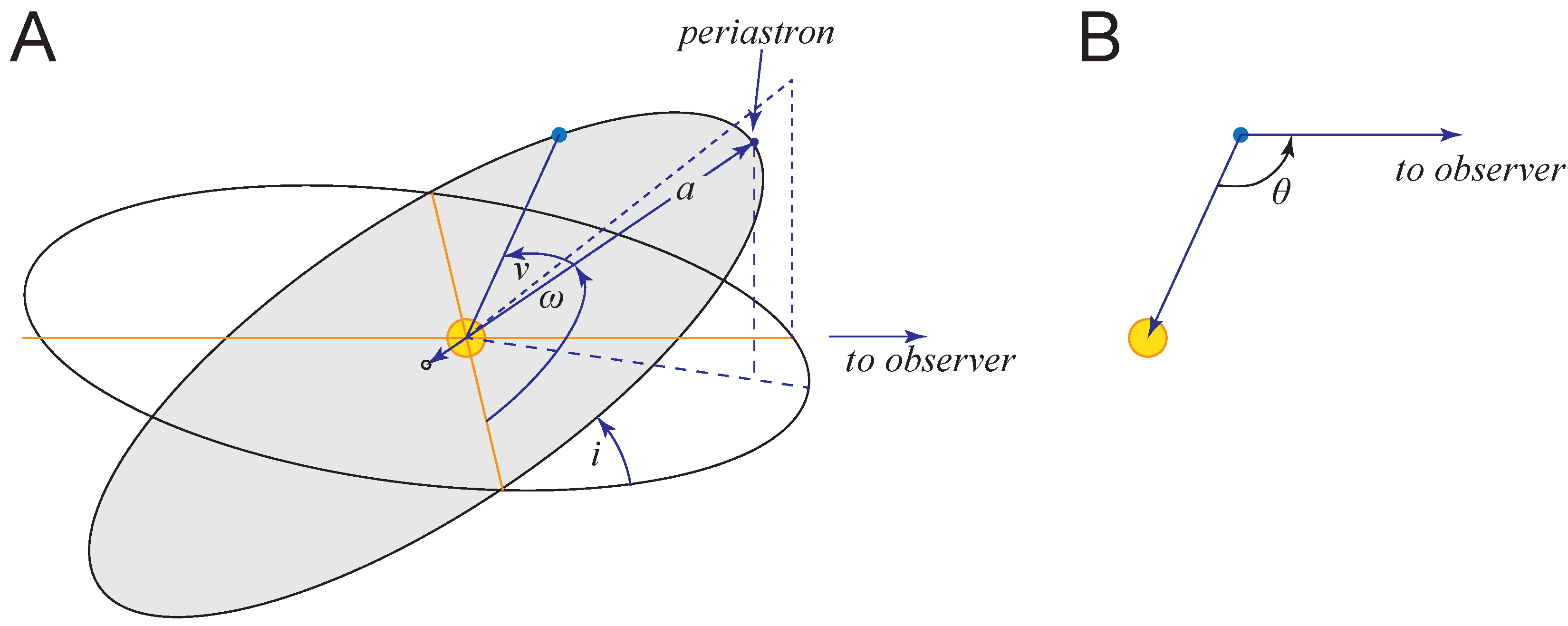
Figure 3.
(A) Light curve of HAT-P-7b recorded by Kepler as processed and published by Borucki et al. [26] (reprinted here with permission). (B) The same light curve at greater magnification. The red line marks the baseline flux. The plot in (C) illustrates the residual, which is the difference between the data and the model. The lack of obvious structure in the residual indicates that most of the effects have been well modeled.

Figure 4.
The range of geometries of a planet illuminated by a star. (A) A planet orbits an average star at a great distance. The star’s rays are more or less parallel, so that one-half of the planet is in illuminated daylight and the other half is in night. (B) A planet in a close-in orbit around a giant star is more than 50% illuminated with a full daylight zone, a penumbral zone and a night zone.
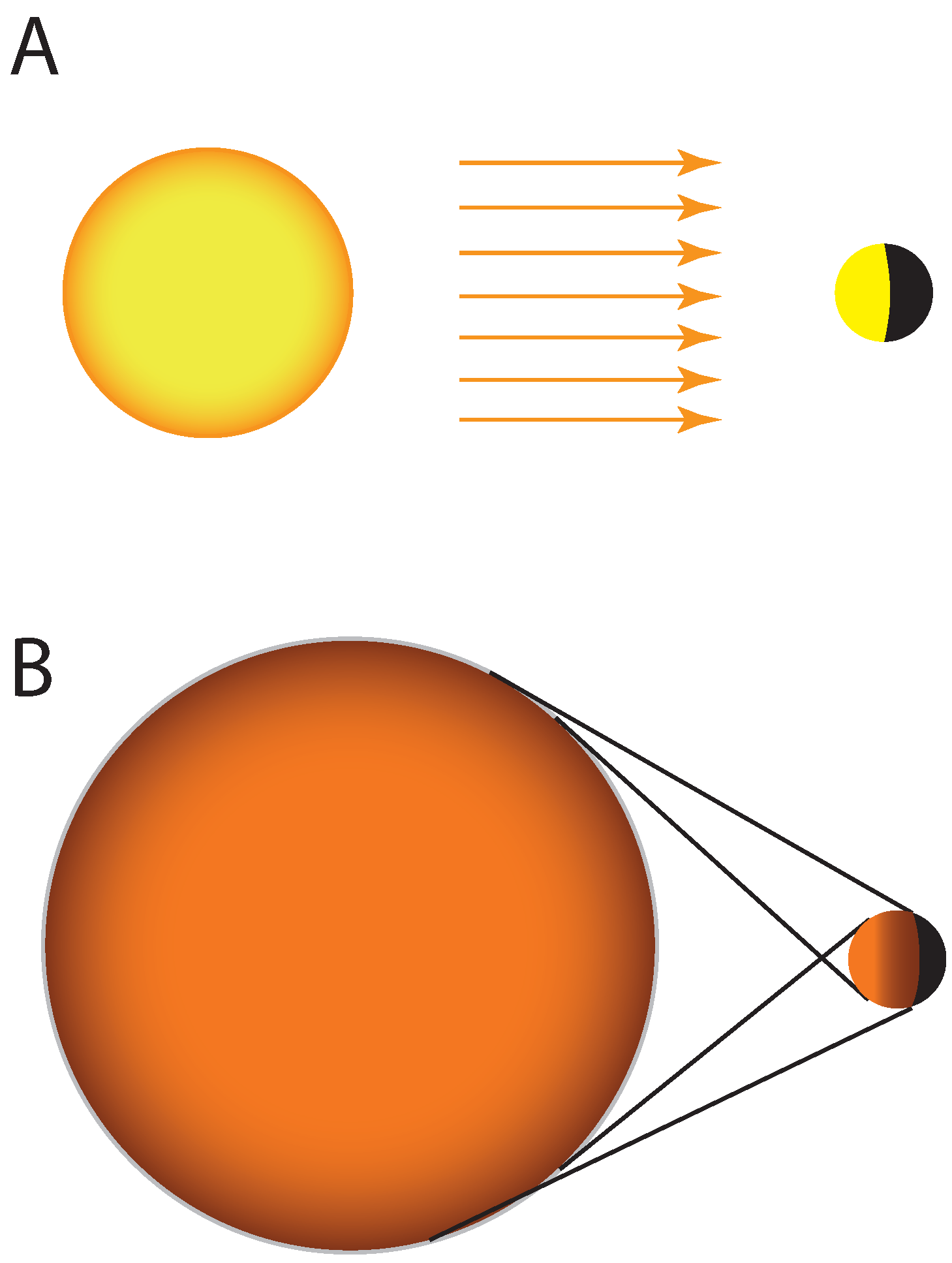
Figure 5.
For 1306 exoplanets in the Exoplanet Archive, this figure shows histograms of the percent of the surface area that is in full daylight, in a penumbral zone and in completely dark night. Note that slightly less than half of the planets have a 50% full daylight zone or a 50% night zone. It is most common for planets to have a 5% penumbral zone, and more than one quarter of the planets have penumbral zones that are larger than 5%. There are four planets with significant penumbral zones in which the full daylight zone covers only about 30% of the surface of the planet.

Figure 6.
(A) This photograph taken by the Cassini space probe of Saturn’s moons Rhea (upper left), Titan (center) and Mimas (lower left) illustrates the role that Titan’s atmosphere plays in changing the illumination of the moon when almost backlit. The illuminated arc is much brighter and more extensive on Titan due to refraction and forward scattering through its significant atmosphere. (B) In the image on the right, Titan is seen in the foreground with Saturn’s rings in the background. Both are backlit in this image, and Titan is surrounded by a brilliant halo of refracted light. Public Domain Images. Credit: NASA/JPL-Caltech/Space Science Institute.
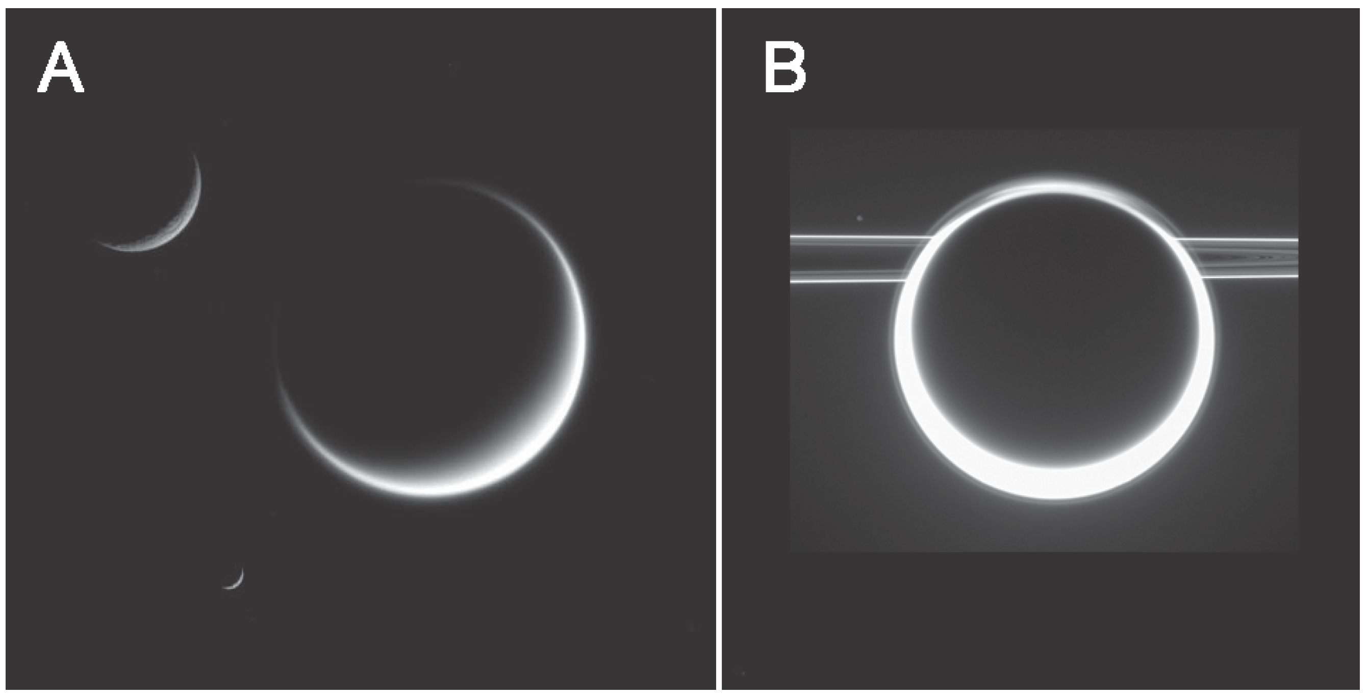
Figure 7.
This is an exaggerated image of a star that has been tidally distorted by a closely-orbiting planet . The increased cross-sectional area results in variations in flux that oscillate at twice the orbital period as the planet revolves around the star.
Figure 7.
This is an exaggerated image of a star that has been tidally distorted by a closely-orbiting planet . The increased cross-sectional area results in variations in flux that oscillate at twice the orbital period as the planet revolves around the star.
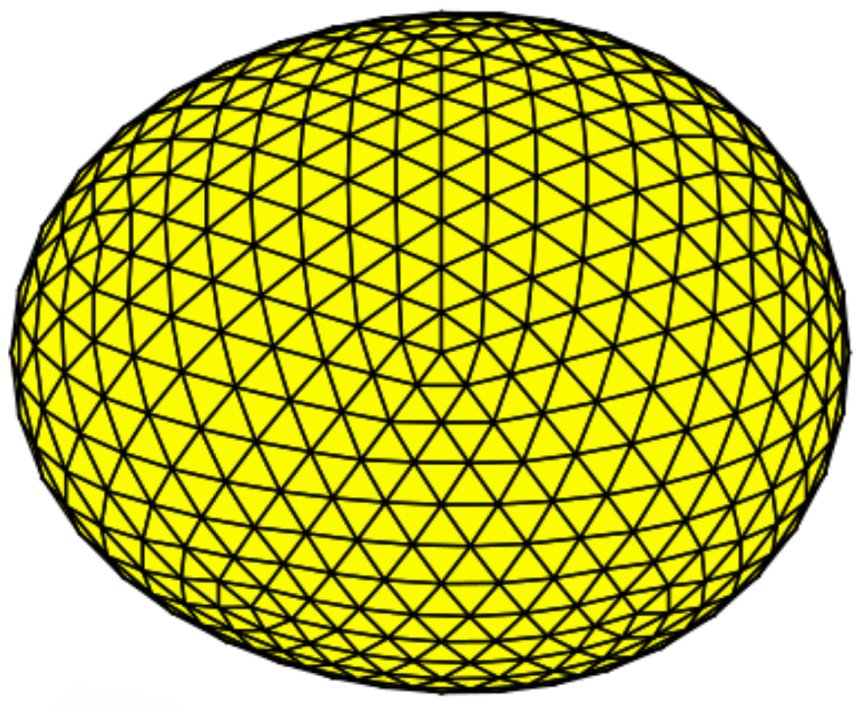
Figure 8.
An illustration of the best fit model (REB + SR) for Kepler-76b. The overall shape of the light curve is due to the reflected light, Doppler boosting and ellipsoidal variations. The secondary eclipse can be observed at an orbital phase of 0.5, which is shifted from the peak of the reflected light component (dashed curve) by 8.53 0.12, which most likely is due to atmospheric superrotation.


Table 1.
This table lists the probability that a distant observer could possibly observe each of these planets transiting the Sun given the semi-major axis of their orbit in astronomical units (AU). These probabilities fall off as as expressed in (12).
Table 1.
This table lists the probability that a distant observer could possibly observe each of these planets transiting the Sun given the semi-major axis of their orbit in astronomical units (AU). These probabilities fall off as as expressed in (12).
| Planet | Semi-Major Axis (AU) | Transit Probability |
|---|---|---|
| Mercury | 0.39 | 1.18% |
| Venus | 0.72 | 0.64% |
| Earth | 1.00 | 0.46% |
| Mars | 1.53 | 0.30% |
| Jupiter | 5.20 | 0.09% |
| Saturn | 9.54 | 0.05% |
| Solar Radius | 0.0046 AU |
Table 2.
This table lists the evidence values obtained by performing model testing with the EXONEST algorithm. The Bayes’ factor is computed by taking the difference between the logarithm of the Bayesian evidence of the model under consideration and the Ellipsoidal Variations Induced by a Low-Mass Companion (EVIL-MC) model. EVIL-MC is slightly preferred over the trigonometric models of Kane and Gelino (Mod) and BEaming, Ellipsoidal and Reflection (BEER).
| Model | Log (Evidence) | EVIL-MC’s Bayes’ Factor |
|---|---|---|
| EVIL-MC | 14,256.91 ± 0.91 | 1 |
| Kane and Gelino (Mod) | 14,256.71 ± 0.73 | 2.20 |
| BEER | 14,256.26 ± 0.74 | 2.65 |
| Kane and Gelino (2012) | 14,253.66 ± 0.72 | 5.25 |
Table 3.
EXONEST model testing results for Kepler-76b. This table lists the log-Bayesian evidence () and maximum log-likelihood values () for model fits of Kepler-76 data. The favored model (listed in bold) incorporates each of the photometric effects plus atmospheric superrotation (reflection, ellipsoidal variations and Doppler beaming (REB)-SR). This model is favored by both the Bayesian evidence and the maximum log-likelihood.
| Model | log Z (×10) | log |
|---|---|---|
| R | −9.5987 | −9.5987 |
| RE | −9.5822 | −9.5822 |
| REB | −9.5685 | −9.5684 |
| REB + SR | −9.5676 | −9.5676 |
Table 4.
EXONEST (REB + SR model) parameter estimate results for Kepler-76b. This table lists the estimated radius, , mass, , orbital inclination, i, and geometric albedo, , of Kepler-76b. These values are comparable to those reported by Faigler et al. using the BEaming, Ellipsoidal and Reflection (BEER) algorithm [80], and Angerhausen et al. [81].
| Kepler-76b Parameter Estimates (REB + SR Model) | ||
|---|---|---|
| Model Parameters | REB + SR Parameter Estimates | Literature Values |
| 1.35 ± 0.05 | 1.25 ± 0.08 | |
| 1.97 ± 0.12 | 2.0 ± 0.26 | |
| i | 77.9 ± 0.03 | 78.0 ± 0.2 |
| 0.31 ± 0.22 | 0.23 ± 0.02, 0.22 ± 0.02 | |
Table 5.
This table lists the modeled effects considered in this paper and indicates which effects are currently implemented (`X’) in EXONEST, and which are currently under development (“D”) or being refined (“R”) or studied (“S”) for potential inclusion in the next generation of our software. Effects marked with an “M” are being or will be evaluated using Bayesian model testing.
| Modeled Effect | EXONEST | Under Study |
|---|---|---|
| Circular Orbits | X | |
| Elliptical Orbits | X | |
| Primary Transit | X | |
| Secondary Eclipse | X | |
| Limb Darkening | X | M |
| Reflected Light | X | R |
| Refracted Light | S | |
| Thermal Emissions | X | R |
| Doppler Beaming | X | |
| Ellipsoidal Variations | X | M |
| Atmospheric Effects | S | |
| Multiple Planets | D | |
| Planetary Shapes | S |
© 2017 by the authors. Licensee MDPI, Basel, Switzerland. This article is an open access article distributed under the terms and conditions of the Creative Commons Attribution (CC BY) license (http://creativecommons.org/licenses/by/4.0/).
Share and Cite
MDPI and ACS Style
Knuth, K.H.; Placek, B.; Angerhausen, D.; Carter, J.L.; D’Angelo, B.; Gai, A.D.; Carado, B. EXONEST: The Bayesian Exoplanetary Explorer. Entropy 2017, 19, 559. https://doi.org/10.3390/e19100559
AMA Style
Knuth KH, Placek B, Angerhausen D, Carter JL, D’Angelo B, Gai AD, Carado B. EXONEST: The Bayesian Exoplanetary Explorer. Entropy. 2017; 19(10):559. https://doi.org/10.3390/e19100559
Chicago/Turabian StyleKnuth, Kevin H., Ben Placek, Daniel Angerhausen, Jennifer L. Carter, Bryan D’Angelo, Anthony D. Gai, and Bertrand Carado. 2017. "EXONEST: The Bayesian Exoplanetary Explorer" Entropy 19, no. 10: 559. https://doi.org/10.3390/e19100559
Note that from the first issue of 2016, this journal uses article numbers instead of page numbers. See further details here.