Detection of Causal Relations in Time Series Affected by Noise in Tokamaks Using Geodesic Distance on Gaussian Manifolds

Abstract

Modern experiments in Magnetic Confinement Nuclear Fusion can produce Gigabytes of data, mainly in form of time series. The acquired signals, composing massive databases, are typically affected by significant levels of noise. The interpretation of the time series can therefore become quite involved, particularly when tenuous causal relations have to be investigated. In the last years, synchronization experiments, to control potentially dangerous instabilities, have become a subject of intensive research. Their interpretation requires quite delicate causality analysis. In this paper, the approach of Information Geometry is applied to the problem of assessing the effectiveness of synchronization experiments on JET (Joint European Torus). In particular, the use of the Geodesic Distance on Gaussian Manifolds is shown to improve the results of advanced techniques such as Recurrent Plots and Complex Networks, when the noise level is not negligible. In cases affected by particularly high levels of noise, compromising the traditional treatments, the use of the Geodesic Distance on Gaussian Manifolds allows deriving quite encouraging results. In addition to consolidating conclusions previously quite uncertain, it has been demonstrated that the proposed approach permit to successfully analyze signals of discharges which were otherwise unusable, therefore salvaging the interpretation of those experiments.

1. Time Series and Causal Relations in Magnetic Confinement Nuclear Fusion

In Magnetic Confinement Nuclear Fusion (MCNF), the largest experiments can produce tens of Gigabytes of data per shot. The JET warehouse nowadays contains more than 400 terabytes of data, which are typically in the form of time series [1]. These time series are the results of measurements performed with systems, called diagnostics, which are typically sub experiments in themselves. The signals produced by diagnostics are affected by significant levels of noise, which can reach 20% or even 30% of their amplitude (10–15% being more normal values). The sources of noise are difficult to reduce and are typically independent. Such uncertainties can complicate significantly the data analysis process, particularly when delicate causal relations have to be investigated.

In recent decades, it has become apparent that, in the future, larger devices, such as ITER (International Thermonuclear Experimental Reactor) and beyond, the control of certain potentially harmful instabilities will have to be stepped up. Two of the major instabilities, which have received a lot of attention lately, are Edge Localised Modes (ELMs) and sawteeth [2,3,4]. ELMs constitute losses of matter and energy at the edge of the plasma column and can reduce significantly the life of the plasma facing components, if allowed to grow excessively. Sawteeth are redistributions of energy and particles from the centre of the plasma column to the more peripheral regions, following magnetic reconnections; if they become too large, they can trigger more harmful instabilities, such as Neoclassical Tearing Modes, which, in their turn, can lead to sudden terminations of the discharges. One route for controlling these instabilities is by pacing, which consists of triggering them frequently enough that they do not have time to reach harmful proportions. One approach to pacing ELMs makes use of ice pellets, injected at the edge of the plasma to destabilise it at predefined appropriate times. In turn, sawteeth can be paced by switching off the Ion Cyclotron Radiofrequency Heating (ICRH) power, therefore reducing the fast ion component, which has a stabilising effect [5,6]. Both pellets and ICRH notches can be considered time localised perturbations of the natural evolution of the plasma.

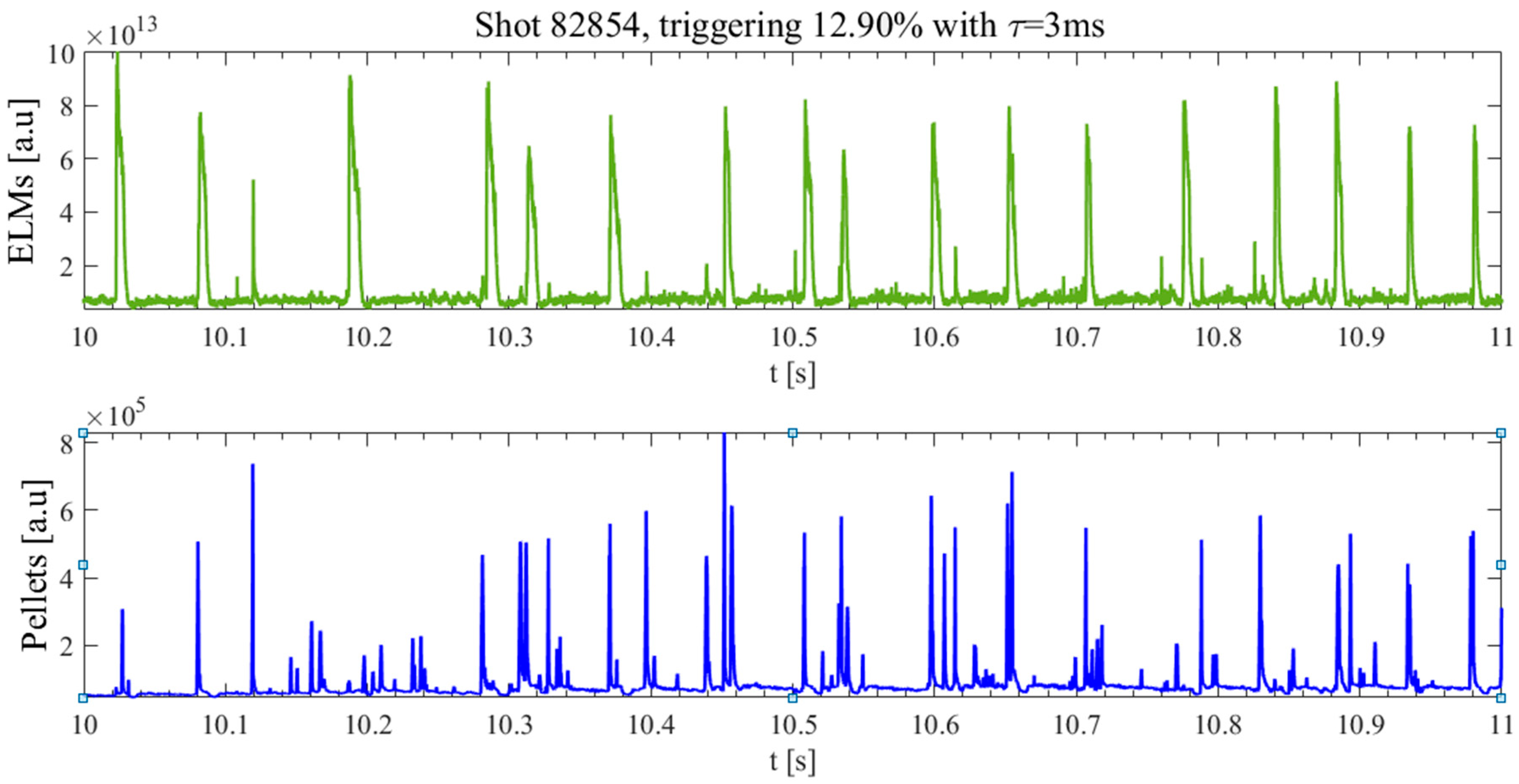
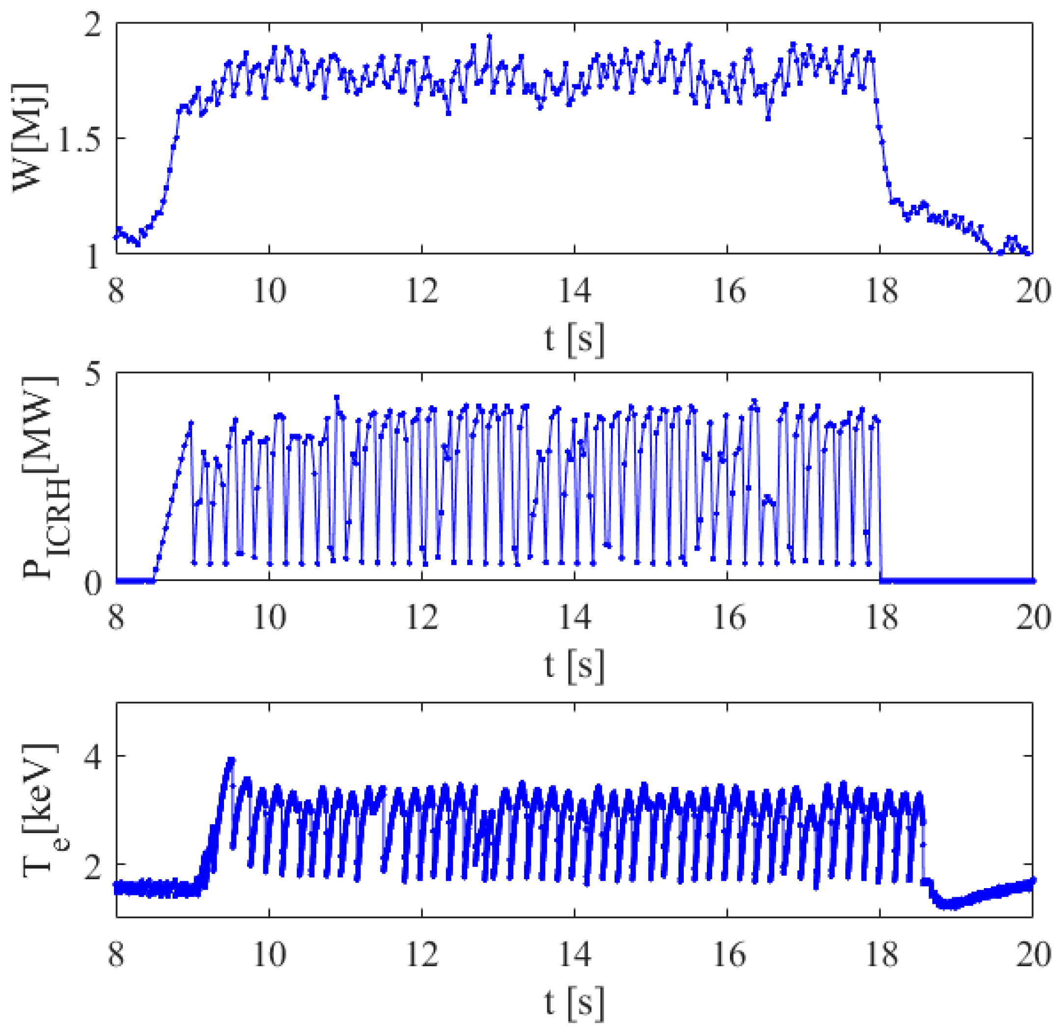
In addition to many practical implementation difficulties, such pacing techniques pose significant interpretation issues. Indeed, both instabilities are quasi periodic and therefore, after the perturbation induced by the control systems, and if enough time is allowed to pass, the instabilities are bound to reoccur. This, of course, renders quite delicate the task of assessing whether an ELM or sawtooth crash has been really triggered by the control system or is the consequence of the natural evolution of the plasma dynamics. How challenging the problem is can be appreciated by inspection of the plots in Figure 1 and Figure 2, where typical case of ELMs pacing with pellets and sawteeth pacing with ICRH modulation are reported.

Given the nature of the experiments and the quality of the available signals, it is not possible to determine the causality at the level of individual perturbations and instability crashes, using only data analysis tools. Since quantitative and adequately validated physics models are not available, an alternative common strategy consists of determining, on the basis of advanced statistical analysis, the time horizon over which the perturbations are effective in triggering the instabilities. The percentage of crashes happening within that time horizon is considered a good estimate of the efficiency of the pacing scheme implemented. Various advanced statistical techniques, such as Transfer Entropy, Granger Causality and Recurrence Plots, have been deployed to address this issue [7]. They have provided very coherent estimates and, since they are mathematically completely independent methods, this convergence of their estimates increases significantly the confidence in the obtained results. On the other hand, in some cases, particularly when the noise is high and/or the plasma reaction to the perturbations is ambiguous, even these advanced techniques cannot provide a clear answer. In order to obtain more robust results about the time horizon of the causal relations also in these difficult cases, it has been tried to handle the signal noise in a more advanced way. Indeed, practically all the techniques deployed are based on the notion of distance. The formulation of distance, traditionally implemented in the calculations of the various methods, is the Euclidean distance, which is very intuitive to understand but is based on a stringent assumption: the points, whose distance is to be determined, are exact values not affected by any uncertainties. This is obviously not verified by JET measurements and therefore it is legitimate to wonder whether a better treatment of the noise could contribute to clarifying the most critical cases. The notion of distance adopted to better handle the measurement noise is based on the information geometric concept of Geodesic Distance on Gaussian Manifolds (GDGM). According to this methodology, the measurements are not considered exact values but probability distribution functions (pdfs) of the Gaussian types. The distance between them is therefore a distance between pdfs. This specific definition of distance has been implemented to analyze the data of the synchronization experiments with the techniques of the Recurrence Plots (RP) and Complex Networks (CN). Whereas RP have been already deployed in the past to analyze data in JET, to our knowledge this is the first case in which CN are applied to MCNF signals.

With regard to the structure of the paper, next section describes the mathematics of RP. The following Section 3 is devoted to the methodology of CN. The concept of GDGM is introduced in some detail in Section 4. Section 5 reports the results obtained applying the proposed techniques to some quite difficult cases of synchronization experiments in JET. Section 6 of the paper is devoted to the discussion and conclusions.

2. Recurrence Plots

In recent decades, recurrence plots have proved to be quite powerful tools for nonlinear data analysis. Dynamical systems can have quite different and distinctive recurrence properties in phase space. Investigating and visualizing the behavior of recurrences in phase space can therefore provide valuable information about the dynamics of a system. In 1987 Eckmann and co-workers introduced a tool, which allows visualizing the recurrence of state x_i even if the dimensionality of the phase space is much higher than two [8]. This is achieved by showing the times at which phase space trajectories visit approximately the same region in phase space. This visualization approach is called Recurrence Plot (RP) and is mathematically expressed by a two-dimensional squared matrix, the so called recurrence matrix:

$$R_{ij}\left(\mathsf{ϵ}\right)=\mathsf{\Theta }\left(\epsilon -||\overrightarrow{y_i}-\overrightarrow{y_j}||\right),i,j=1,\dots ,N$$

(1)

where N is the number of considered samples y_i, ε is a threshold distance, ||·|| a norm and Θ(·) is the Heaviside function. Each element indicates the recurrence of a state at time i at a different time j, equal to one if the distance between the two states is lower than ε, and equal to zero otherwise. A graphical representation of a RP is obtained by plotting the matrix in a square map, whose axes report time and black dots indicate ones and white dots zeroes.

In our application, the objective consists of investigating the coupling between two dynamical systems and therefore multivariate extensions of recurrence plots are required. The version, adopted to obtain the results reported in the rest of the paper, is the joint recurrence plots (JRP). Joint recurrence plots are the Hadamard product of the recurrence plots of the considered systems [9], e.g., for two systems x and y the joint recurrence plot is:

$$JR\left(i,j\right)=\Theta \left({\epsilon }_x-||\overrightarrow{x_i}-\overrightarrow{x_j}||\right)\times \Theta \left({\epsilon }_y-||\overrightarrow{y_i}-\overrightarrow{y_j}||\right),i,j=1,\dots ,N$$

(2)

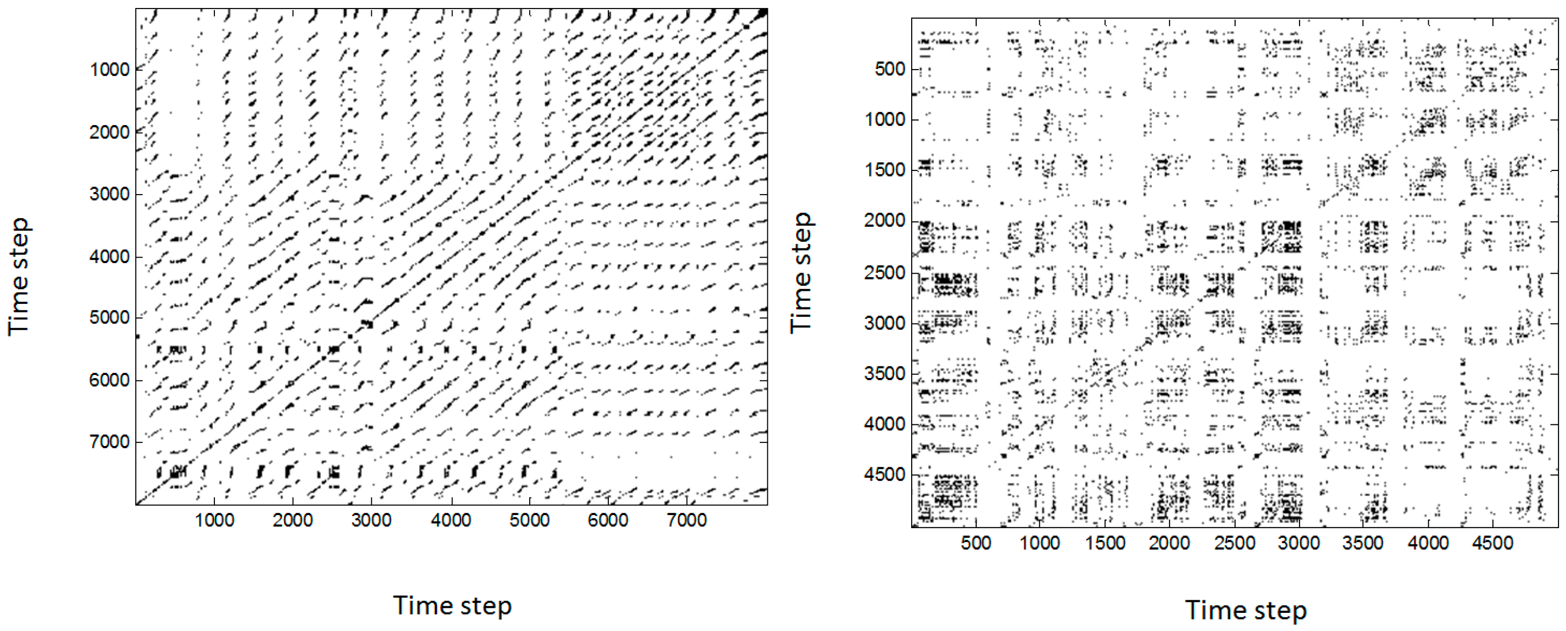
In contrast to cross recurrence plots, joint recurrence plots compare the simultaneous occurrence of recurrences in two (or more) systems. Two examples for two discharges studied in this paper are reported in Figure 3. To interpret the visual features present in RPs, it should be considered that single isolated points correspond to states occurring rarely, which do not persist in time and are characterized by high fluctuations. Vertical and horizontal lines indicate states which do not change significantly in a certain period of time. On the other hand, diagonal lines occur when the trajectory visits the same region at different times. The length of a diagonal is proportional to the duration of this similar local evolution of the trajectories. As, by definition, $JR\left(i,i\right)=1$, a black main diagonal, with an angle of $\pi /4$, called line of identity (LOI), always appears and has no physical meaning. In case of two processes, analyzed by means of JRPs, the long diagonal structures indicate similar time evolutions of the two processes. From the plots of Figure 3, it can be seen how the signals of the Dα, due to the ELMs, show a faster and noisier dynamics than the on-axis electron temperature affected by sawteeth.

It is worth noting that the basic definitions of RP and JRP imply the calculation of a distance. In practically all applications reported in the literature, this norm is the Euclidean distance. In this paper, the Euclidean distance has been replaced by the GDGM (see Section 4) to address the issue of the influence of the noise and to see whether a more appropriate metric can improve the causality detection.

RPs and JPRs not only allow a useful visualization of the recurrences but permit also to quantify very important properties of a system phase space. The field of deriving quantitative indicators about the dynamics from recurrence plots is called Recurrence Quantification Analysis (RQA). RQA is based on the distributions of the diagonal, horizontal and vertical lines that are found in the RPs [9,10]. Of particular relevance for the subject of this paper is the entropy of the diagonal length, defined as the Shannon entropy of the frequency distribution of the diagonal lengths:

$$ENTR={\displaystyle \sum }_{l=l_{min}}^{N}p\left(l\right)lnp\left(l\right)$$

(3)

where

$$p\left(l\right)=\frac{P\left(l\right)}{{{\displaystyle \sum }}_{l=l_{min}}^{N}P\left(l\right)}$$

(4)

and $p\left(l\right)$ is the frequency distribution of the lengths l of the diagonal lines. In other words, ENTR is the Shannon entropy of the probability $p\left(l\right)$ to find a diagonal line of exactly length l in the RP. The entropy gives a measure of how much information is needed to recover the system and it reflects the complexity of the RP with respect to the diagonal lines. For uncorrelated noise the value of ENTR is rather small, indicating its low complexity. It is to be noted that, as discusses in detail in the references [5,7], the indicator ENTR assumes a maximum at the times of the highest causal interaction between the signals.

3. Complex Networks

Many systems of interest to scientists can be modelled as individual parts connected by suitable links. The pattern of connections in such systems is the field of study of network science [11]. Most sociological and technological systems have patterns of interactions, which present non-trivial topological properties. In particular, the distribution of the links is neither random not fully regular but can show quite complex structures. Two important and quite popular types of complex networks are the scale-free networks and small-world networks. Complex networks are able to provide profound insights into many complicated systems in engineering, social and biological fields [12]. Mathematically one important representation of networks is based on the intuitive and convenient adjacency matrix. The elements of the matrix indicate if pairs of nodes are connected or not. It can be defined by the following relation:

$$A_{ij}=\{\begin{array}{c}1,\mathrm{if}\mathrm{nodes}i\mathrm{and}j\mathrm{are}\mathrm{connected}\\ 0,\mathrm{otherwise}\end{array}$$

If the link between the nodes is two-way then $A_{ji}=A_{ij}$. A network with all two-way links is called undirected and, in this case, the adjacency matrix is symmetric.

Complex networks have been used as a new framework for exploring the dynamics of time series. By means of specific transformations from the time domain to the network domain, the dynamics of the time series can be studied via the organization of the network by using topological statistical measures. The first approach to convert time series data into complex networks has been proposed by Zhang et al. [13]. It consists of constructing a network from pseudo periodic time series, where each cycle is represented by a single node and a threshold is set to link node pairs with strong cross-correlations.

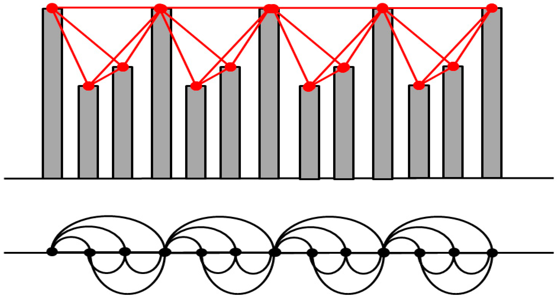
A widely used approach, called visibility graphs (VG), has been reported recently by Lacasa et al. [14] and is inspired by the concept of visibility [15]. Considering a representation of time series by using vertical bars and seeing this representation as a landscape, every bar in the time series is linked with those that can be seen from the top of the bar (Figure 4). Each point in the series is assigned to a node in the VG. Two points in the time series ($t_i,y_i$) and ($t_j,y_j$) will be connected if a straight line connecting the amplitudes of the two points is always higher than the amplitudes of all the points in between. Mathematically, for any intermediate point ($t_k,y_k$), this condition translates into the following relation:

$$y_k<(y_j-y_i)\frac{t_j-t_k}{t_j-t_i}$$

(5)

VGs are connected, undirected and invariant under affine transformation but also “lossy” as some information regarding the time series is inevitably lost in the mapping–two different time series may produce the same VG as noticed in [16]. However, most of the time series structure is inherited in the VG; for example periodic, random and fractal series map into motif-like, random exponential and scale-free networks, respectively [17]. This suggests that the VGs are able to capture the dynamical fingerprints of the process that generated the series.

While the visibility graph represents a novel view for analysing time series, the recently introduced “cross-visibility” networks (CVN) reveals the possible coupling between them [18]. This is the technique used in the rest of the paper, since our objective is to investigate the causal relation between typically two different signals (see Section 5 for the details about the nature of the signals). The mapping of the time series into a complex network is constructed in two steps. First the nodes on the network are defined by a biunivoc correspondence with the points of the time series. Then the connection of nodes $i$ and $j$ is established if one of the following relations are valid:

$$y_k\le y_i+\frac{x_j-x_i}{j-i}\left(k-i\right),i<\forall k<j$$

(6)

$$y_k\ge y_i+\frac{x_j-x_i}{j-i}\left(k-i\right),i<\forall k<j$$

(7)

According to (6) and (7), node $i$ in time series $\left\{y_j\right\}$ is looking at the components of $\left\{x_j\right\}$ time series, through the obstacles defined by the shifted time series $\left\{y_j\right\}$ = {$y_j$ − $y_i$ + $x_i$}. Equation (6) accounts for the visibility from the top view, while Equation (7) accounts for the visibility from the beneath view. Basically the top view is determined by the reciprocal visibility of the peak values of the time series, whereas the beneath view by the reciprocal visibility of the valleys. The network constructed in this way has an adjacency matrix with unit values for the cases when the relations (6) and (7) are satisfied and 0 otherwise.

Based on these definitions, topological measures-like e.g., clustering coefficient, average path length and node degree distribution-can be applied for investigating the structural patterns characterising the network and implicitly the time series [19]. However, these types of measures do not take into account the presence of noise in the data. Additional measures have therefore to be devised in order to allow correction methods to be implemented. In this perspective, we have modified the network adjacency matrix by weighting the connections with the metric distance between two connected values in the time series:

$$A_{ij}=\{\begin{array}{c}dist\left(y_i-y_j\right),\mathrm{if}\mathrm{either}\mathrm{Equation}\left(6\right)\mathrm{or}\mathrm{Equation}\left(7\right)\mathrm{is}\mathrm{satified}\\ 0,\mathrm{otherwise}\end{array}$$

(8)

The metric distance $dist$ in the relation above is the GDGM and therefore it takes explicitly into account the presence of noise in the input data. The structural complexity of the Weighted Cross Visibility Graph (WCVG) can be evaluated by using the Shannon entropy of the normalized adjacency matrix:

$$S=-{\displaystyle \sum }_{i,j}{A}_{ij}ln{A}_{ij}$$

(9)

A reduced number and length of the paths in the visibility graphs corresponds to a network with reduced complexity and to a lower value of the entropy. For coupled time series, this happens when the time series are not synchronized and the visibility of two points in the time series $\left\{y_k\right\}$ are more frequently interrupted by obstacles in the time series $\left\{x_i\right\}$. Therefore, as in the case of the Entropy of diagonal lengths calculated for the RP, also the indicator WCVG presents a peak at the time lags of the highest level of causal interaction between the time series.

4. Information Geometry: Geodesic Distance on Gaussian Manifolds

As seen in the previous sections, several indicators, used to assess quantitatively the results of recurrent plots and complex networks, are based on some sort of distance. This applies also to entropy-like quantifiers. In more traditional applications, the Euclidean distance metric is adopted to calculate such distances. This choice is based on the assumption that the time series to be analyzed consist of a succession of infinitely precise values. This hypothesis is obviously not satisfied in the case of plasma physics, particularly in large Tokamaks, whose diagnostics can produce measurements affected by significant errors, up to 20% or 30% of the measured values. Therefore, a more suitable metric is required to quantify the results of recurrent plots and complex networks. In this perspective, it should be considered that in Tokamaks the measurements are affected by a wide range of noise sources, which statistically can be considered independent random variables. Therefore, the noise can reasonably be expected to lead to measurements with a global Gaussian distribution around the most probable value, the actual value of the measured quantity. Such an experimental situation justifies considering the measurements not as points, but as Gaussian distributions. Each measurement can therefore be modelled as a probability density function of the Gaussian type, determined by its mean μ and its standard deviation σ.

Considering the measurements not as punctual values in the Euclidean space, but as Gaussian distributions, requires defining a distance between Gaussians. In the mathematical field of information geometry, the analysis of distances between probability density functions [20] has been investigated in detail. In particular, the various families of pdfs can be considered as lying on a Riemannian differential manifold. A point on this manifold corresponds to a specific pdf and the Fisher information constitutes a metric tensor (Fisher–Rao metric) on such manifold [21]. It can be demonstrated that the Fisher–Rao metric is a unique intrinsic metric on such a manifold and is invariant under basic probabilistic transformations. In the case of Gaussian pdfs, the most appropriate distance is the Geodesic Distance on the Gaussian Manifold (GDGM) containing the data, which can be calculated using the Fisher–Rao metric. For two univariate Gaussian distributions $p_1\left(x|{\mu }_1,{\sigma }_1\right)$ and $p_2\left(x|{\mu }_2,{\sigma }_2\right)$, parametrized by their means ${\mathsf{\mu }}_1$ and standard deviations ${\sigma }_i$, the geodesic distance GDGM is given by:

$$\mathrm{GDGM}(p_1||p_2)\sqrt{2}Ln\frac{1+\delta }{1-\delta }=2\sqrt{2}tan{h}^{-1}\delta ,$$

(10)

$$\mathrm{where}\delta ={\left[\frac{{({\mu }_1-{\mu }_2)}^2+2{({\sigma }_1-{\sigma }_2)}^2}{{({\mu }_1-{\mu }_2)}^2+2{({\sigma }_1+{\sigma }_2)}^2}\right]}^{1/2}.$$

(11)

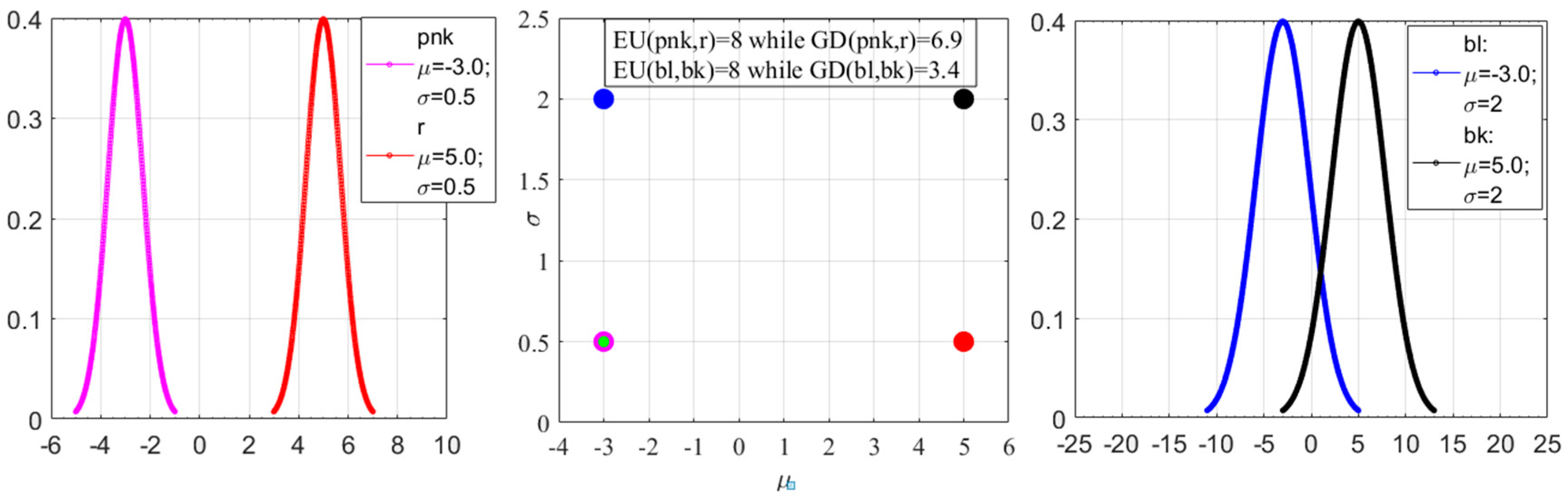
Contrary to the Euclidean distance, the GDGM respects the intrinsic geometry of the Riemannian manifold on which the pdfs lie. The properties of the GDGM can be appreciated by inspecting Figure 5, which reports the distance between two couples of Gaussian distributions: P₁ Q₁ (pink and red in Figure 5) and P₂ Q₂ (blue and black in Figure 5). The distance between the means of the members of the two couples is the same. On the other hand, the Gaussian pdfs P₁ Q₁ have a standard deviation about an order of magnitude smaller than the other couple. The distance between the pdfs with higher standard deviation, P₂ Q₂, is therefore significantly lower than the one of the more concentrated pdfs. Inspection of Figure 5 reveals the meaning of this fact, since there is a much larger overlap between the P₂ Q₂ pdfs and therefore it is appropriate to consider them closer than the two of the other couple.

5. Application of the Geodesic Distance to Synchronization Experiments in JET

The estimators introduced in the previous sections have been applied to JET discharges. The time of maximum causal influence between time series is found by varying the delay between the time series and calculating the evolution of the entropy of diagonal lengths for RP (Equation (3)) and of the Shannon entropy of the adjacency matrix (Equation (9)) in case of WCVG. For synchronized time series, RP and WCVG develop a more complex structures and therefore the maximum causal influence is associated with a peak in the evolution of these estimators [5,7].

The signals used to build the JRP and the WCVG are: (a) for the ELM pacing the Dα signals of the pellets and the ELMs (b) for the sawteeth pacing the ICRH power and the central electron temperature. The approach of the GDGM introduced in the previous section is predicated on the assumption that the noise of the used signals, the Dα and the temperature measured from the Electron Cyclotron Emission (ECE), are affected by noise of Gaussian distribution. The hypothesis of noise gaussianity is more than reasonable given the nature of the physical processes generating the signals. The Dα signal consists of radiation emitted from a series of atomic processes taking place at the plasma edge. Therefore the Dα is affected not only by instrumental noise but even more by internal dynamic noise. The same considerations apply, even if less severely, to the signal of the electron temperature. The ECE measurement is affected by significant thermal and magnetic fluctuations. Therefore, given the plurality of the noise sources, which are independent and at least partly related to thermal fluctuations, it is a very reasonable to assume that the noise presents a Gaussian distribution, as confirmed by the experts of the diagnostics. To obtain the results reported in the following, in the GDGM the value of σ has been set to 15% of the signals amplitude. This is the value suggested by the diagnosticians responsible for the measurements to best model the noise standard deviation. A scan of σ has been also performed, within the reasonable range of 5–30% of the signal amplitude, and indeed the best results have been obtained for the 15% case.

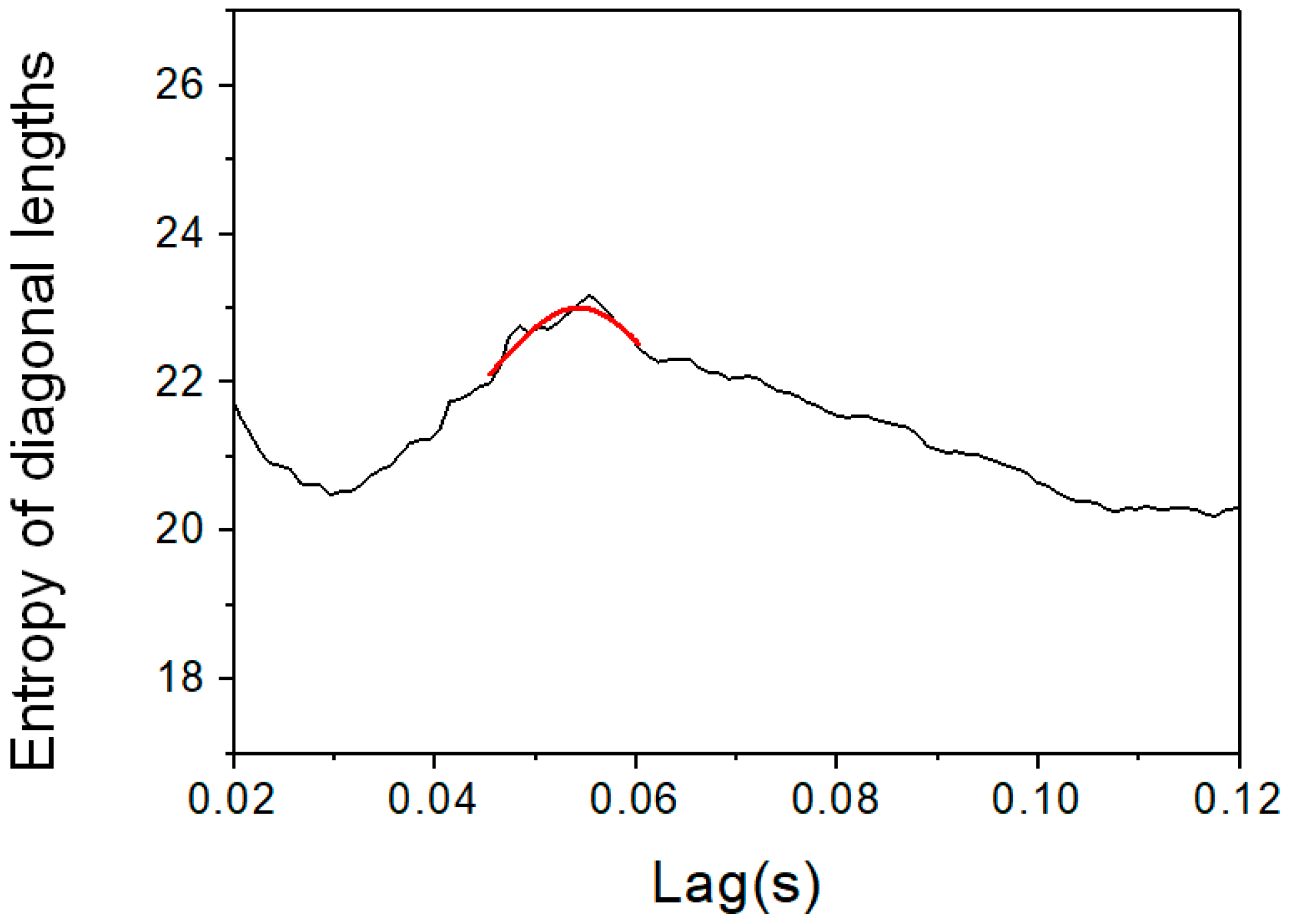
The difficulties inherent to the synchronization analysis of the JET diagnostic signals reside in a set of specific limitations. The peaks, corresponding to events in the signals, have irregular shape. The total number of events is usually limited to a few tens. Moreover, as already mentioned, both ELMs and sawteeth are quasi periodic in nature and therefore, after any pulsed perturbation, if enough time is allowed to elapse, they always occur in stationary discharges. Therefore, the evolution of the synchronization estimators shows peaks with low amplitude. A typical example is presented in Figure 6.

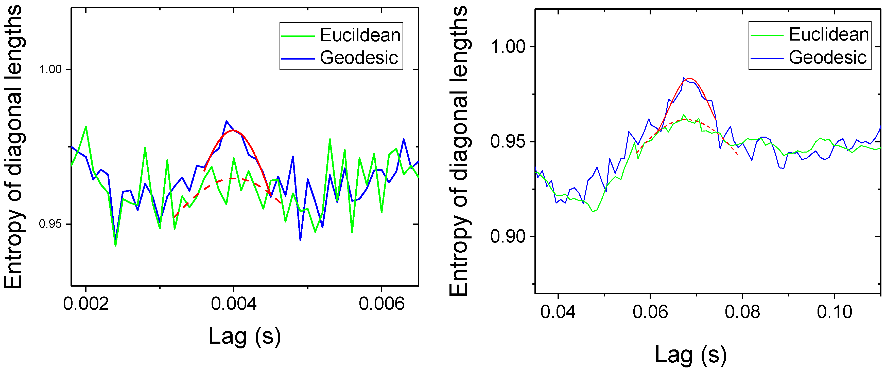
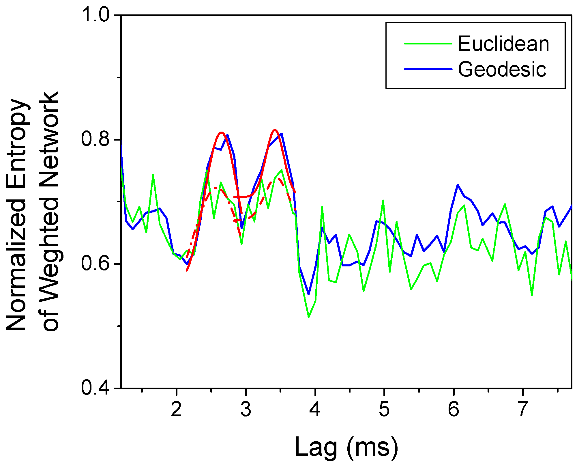
As already discussed, the signals are also inherently affected by a significant level of noise, which may blur the peaks indicating the synchronization. Relevant examples are presented in Figure 7 and Figure 8, where the green curves shows the evolution of the entropies defined in (3) and (9) and calculated using the traditional Euclidean distance. In the case of Figure 7 left plot, it is practically impossible to identify a clear peak in the indicator, the Entropy of diagonal lengths; therefore no clear estimate of the causality horizon can be derived. A similar situation presents itself in Figure 7 right plot and Figure 8, where some sort of peaks can be detected but with really poor level of confidence. On the other hand, the application to these cases of the Geodesic Distance on Gaussian Manifolds, the specific metric defined in Section 4 (Equations (10) and (11)), improves significantly the results. The obtained estimates are presented in Figure 7 and Figure 8 as blue curves. The plots of the two figures show that the use of the geodesic distance makes possible the identification of distinct peaks corresponding to synchronization, whose locations can be defined with sufficient precision. For the shot of Figure 8, a complex example of ELM triggering with pellets, the implementation of the GDGM allows identifying two peaks in the Entropy of the network, proving how the proposed method can resolve different phases in the behavior of non-stationary discharges. To conclude, it is worth pointing out that, for the cases reported in Figure 7 and Figure 8, without the use of the GDGM it would be impossible to obtain any reliable conclusions. Given the chronic shortage of good synchronization experiments on JET, providing clear results for a few more discharges is to be considered extremely valuable.

It is worth pointing out that it has been verified to what extent the approach of the GDGM has better performance than other strategies. In particular, a possible alternative would consist of filtering the signals and then applying the traditional version of the RQA indicators, using the Euclidean distance, to the denoised time series. The two approaches have been compared using a series of synthetic signals, generated by various dynamical systems, to which Gaussian noise of levels relevant to the present applications has been added. The percentage difference between the RQA indicators, calculated using clean data and those calculated using noisy data, has always been in favor of the use of the geodesic distance. For the particular case of the entropy of diagonal lengths for a Lorenz-84 time series, the reduction in the percentage difference with respect to the case of the clean data is of a factor of two (from about 10% to about 5%).

With regard to some more specific computational aspects, it is worth mentioning that, for the construction of the recurrence plots, the embedding dimension is typically determined with the method of the “False Neighbours” [22]. The RP analysis has been performed using the ‘CRP toolbox for Matlab’ [23]. The source code has been modified in order to implement the use of the geodesic distance.

6. Discussion, Conclusions and Future Perspectives

In this paper, a more advanced metric, the GDGM, has been used in the analysis of the causal relation between time series. The main advantage of this distance consists of treating in a sound way the noise associated with the measurements. The application of such a metric to some synchronization experiments on JET has proved to be valuable. For some difficult cases, even the most advanced techniques for the investigation of dynamical systems, such as Recurrence Plots and Complex Networks, struggle to identify a clear time horizon for the causal influence, if the traditional Euclidean metric is adopted. On the other hand, much clearer results are obtained with the GDGM. It is worth pointing out that the combination of GDGM and RP was already pioneered in [24] even if in a completely different context; the combination of CN and GDGM on the contrary is new development reported for the first time in this paper.

The estimates obtained with the approach proposed in this paper are coherent with the previous ones already reported in the literature. The newly reported values therefore support previous conclusions [5,7] and increase the confidence in them. In particular, for the sawteeth pacing with ICRH modulation, it has been confirmed that the slowing down time of the ions is the crucial physical quantity to interpret the experiments [6]. Conversely, it should be mentioned that the examples of sawteeth pacing shown refer to L mode plasmas. In H mode configurations, the effects of the modulation are expected to be less clear and their interpretation will very likely require the systematic deployment of the techniques proposed in this paper. With regard to ELM pacing, the capability to consolidate the conclusions on dubious cases is considered particularly important. Indeed the minimization of the pellet size is a crucial aspect in the future deployment of the pacing, to reduce fuelling and to allow more flexibility in optimizing the scenarios for performance. Of course determining the effects of smaller pellets can be more challenging. Therefore, the approach presented in this paper could significantly contribute to increasing the statistical basis of the results for the interpretation of such experiments.