Thermodynamic Analysis for Buoyancy-Induced Couple Stress Nanofluid Flow with Constant Heat Flux


1
Department of Mathematical Sciences, Redeemer’s University, Ede 232101, Nigeria
2
Department of Mathematics, Vaal University of Technology, Vanderbijlpark 1911, South Africa
3
Department of Mathematics, University of Lagos, Lagos, Nigeria
4
Department of Physics, Redeemer’s University, Ede 232101, Nigeria
*
Author to whom correspondence should be addressed.
Entropy 2017, 19(11), 580; https://doi.org/10.3390/e19110580
Submission received: 20 September 2017
/
Revised: 14 October 2017
/
Accepted: 17 October 2017
/
Published: 29 October 2017
(This article belongs to the Special Issue Entropy in Computational Fluid Dynamics)
Abstract
:This paper addresses entropy generation in the flow of an electrically-conducting couple stress nanofluid through a vertical porous channel subjected to constant heat flux. By using the Buongiorno model, equations for momentum, energy, and nanofluid concentration are modelled, solved using homotopy analysis and furthermore, solved numerically. The variations of significant fluid parameters with respect to fluid velocity, temperature, nanofluid concentration, entropy generation, and irreversibility ratio are investigated, presented graphically, and discussed based on physical laws.
1. Introduction
A striking feature of nanofluids is the inclusion of nanosized metallic particles with high thermal properties to a working base fluid to enhance their thermal properties. Commonly used nanoparticles are gold (Ag), aluminum (Al), copper (Cu), and their oxides. Interestingly, Cu is usually used in many energy conversion processes because it is abundant in nature and inexpensive. At the forefront of these findings is the pioneering work done by Choi [1] on the heat transfer enhancement of fluids with low thermal conductivity. Subsequently, Sheikholeslami et al. [2] performed an analysis to enhance the flow and thermal structure in rotating systems. A similar investigation was also conducted by Sheikholeslami et al. [3] for a magnetohydrodynamic Cu–water nanofluid in a cylindrical passage. Also, Das [4] investigated the radiative magnetohydrodynamic flow over a stretching sheet subjected to slippage. In a study by Heris et al. [5], a Cu–water nanofluid in a tube was examined. Sheikholeslami and Ganji [6] considered the heat transfer of a squeezed Cu–water nanofluid channel flow. Domairry and Hatami [7] analysed the Cu–water nanofluid channel flow using the Maxwell–Garnetts and Brinkman models. Das et al. [8] presented the radiative hydromagnetic buoyancy-induced flow and heat transfer of a Cu–water nanofluid. Hayat et al. [9] investigated the steady MHD Cu–water nanofluid flow on a rotating porous disk. In all the above studies, the Newtonian constitutive model has been used to describe the rheological properties of the fluid. In general, due to technological advancements, there are huge applications for non-Newtonian nanofluids that show more complex rheological properties. In the mechanical engineering and thermal community, for instance, Nadeem and collaborators introduced the wave concept in the study of a couple stress fluid that contains nanoparticles in order to explain arterial flow [10]. Similarly, an analysis was performed for stagnation point flow over a stretching sheet [11]. Furthermore, Awais et al. [12] considered couple stress nanofluid fluids in a vertical configuration and subjected them to Newtonian heating. Hayat et al. [13] presented a comprehensive analysis of magnetohydrodynamics using the couple stress nanofluid concept. More recently, Hayat et al. [14] examined the hydromagnetic flow of squeezed couple stress nanofluids through a channel.
The unavailability of energy has been a major challenge in the energy industry globally, as a good percentage of the energy generated is dissipated as heat in transport. Therefore, since heat transfer processes are irreversible, the place and role of entropy generation minimization in the nanofluid flow and heat transfer cannot be over-emphasized in energy conservation and management. Based on this, Bejan [15,16] used the second law of thermodynamics to describe the minimization of entropy generation in an irreversible process by accounting for the component and sub-component that depletes the available energy for work. Also, Ibáñez et al. [17] reported the global entropy in a radiative nanofluid flow through a micro-channel with slippage. Hussain et al. [18] investigated MHD mixed convection and entropy generation under an inclined magnetic field. The forced convective flow of CuO–water nanofluids that filled the lid-driven cavity with inclined magnetic fields was investigated in [19]. Kefayati [20] studied heat transfer and entropy generation analysis for free convective non-Newtonian nanofluid in a square cavity. Fersadou et al. [21] studied the entropy generation in radiative MHD convective heat-generating nanofluid flow in a porous channel. Hossein et al. [22] studied the entropy analysis for a transient MHD nanofluid flow over an accelerating stretching permeable membrane. Cho [23] investigated the entropy generation in hydromagnetic convective Cu–water nanofluid flow in a cavity with complex-wavy surfaces. More recently, Chen et al. [24] reported on an MHD water–alumina nanofluid through a vertical channel. Interested readers can read more on recent works with or without entropy generations in [25,26,27,28,29,30,31,32,33,34] and the references therein.
Motivated by the study in [25], the specific objective of the present study is to examine entropy generation in the convective flow of couple stress nanofluid with thermophoretic, Brownian motion and constant heat flux in consideration. There are several applications of the present study in mechanical and thermal engineering, for instance, in the crude pyrolysis and heating of other biomass and bioenergy processes. The mathematical problem under discussion is coupled and nonlinear as presented in the model formulation in Section 2. By using a convergent series solution, we obtain a reliable approximate solution for both dimensionless velocity and temperature equations which are presented in Section 3. Entropy generation analysis is presented in Section 4 of the paper. In Section 4 numerical results and discussion are presented, while Section 5 concludes the work.
2. Mathematical Analysis
Consider the convective flow of an incompressible electrically-conducting couple stress nanofluid through a vertical channel of width h apart as shown in Figure 1. The vertical channel is subjected to constant heat flux in one part of the channel and is cooled at the other wall. The present study is done in the presence of a transversely imposed external magnetic field of strength which is applied parallel to the y-axis. The magnetic Reynolds number and the induced electric field are assumed to be small and negligible.
Therefore, the equations governing the fluid flow are as follows:
The non-slip and the non-moving walls, as well as the stress-free and surface constant heat fluxes are given by:
where is the axial velocity, is the fluid density, is the scale of suction velocity, P is the pressure, is the dynamic viscosity, is is the fluid particle size effect due to couple stresses, is electrical conductivity, g is the acceleration due to gravity, is the volumetric coefficient of thermal expansion, is the coefficient of concentration expansion, T is the fluid temperature, is is the ambient temperature, C is the fluid concentration, is the ambient fluid nanoparticle concentration, k is the thermal conductivity, is the specific heat, is the ratio of the heat capacity of the fluid of the nanoparticle material to the effective heat capacity of the base fluid, is the chemical molecular diffusivity of the species concentration, is the thermophoretic diffusion, is the uniform volumetric heat heat generation/absorption coefficient, and is the constant heat flux.
Introducing the following dimensionless parameters and variables,
Equations (2)–(4) then become
where denotes couple stress inverse parameter, G is the modified pressure gradient, H stands for the magnetic field intensity parameter, the thermal Grashof number, stands for the solutal Grashof number, is the Schmidt number, is the thermophoretic parameter, is the Brownian motion parameter, denotes the constant heat source parameter, is the Prandtl number, and is the Brinkman number.
3. Entropy Analysis
The local entropy generation rate per unit volume can be expressed as:
Equation (10) can be written in dimensionless form as:
Let
Then is the heat transfer irreversibility and is the fluid friction irreversibility, while is the diffusive irreversibility. The Bejan number (Be) which represents the ratio of the heat transfer irreversibility to the total entropy generation is given as:
4. Methodology of Solution
We propose a series of analytical solutions for the system of coupled nonlinear differential Equations (6)–(8) subject to the boundary conditions of Equation (9) via the homotopy analysis method (HAM) as described in [35,36]. To solve (6)–(8) we choose the initial approximation estimates , and as follows:
which satisfies the boundary conditions of Equation (9), and the linear operators , and are also defined as:
with the properties
where are the arbitrary integration constants determined from the boundary conditions. If denotes an embedding parameter, and , and are the non-zero parameters, then the zeroth order deformation problems are:
Subject to the conditions
where , and are the nonlinear operators defined as follows:
for p = 0 and p = 1 we have
When p variation is taken from 0 to 1, then , and approach , and , becoming , and . Now, expanding , and in Taylor’s series with respect to p yields the following:
where
By proper choice of the auxiliary linear operator, initial guess and auxiliary parameter, the series above converge from p = 1 and hence
is the one of the solutions of the original nonlinear equation, as proved by [35]. The nth order deformation is
subject to the boundary conditions:
and
The general solution of equations are given by:
where , and are the particular solutions. Constants are determined by the boundary conditions equation.
With the help of symbolic packages such as MATHEMATICA or MAPLE, Equations (34)–(37) can be solved one after the other in the order . All computational work in this present study has been carried out by utilizing symbolic software MAPLE 18, running on an intel fifth-generation computer of 6G RAM. The above computational work may take quite a long solution time mainly due to the lengthy series solution. For example, it takes 8733.484 CPU time for the computation of the 15th-order approximation.
5. Convergence of the HAM Solution
The convergence of the homotopy solution strongly depends on the values of the auxiliary parameters , and . These parameters are used to control the convergence region of the HAM solution. To choose the admissible range for these parameters, the curves are plotted for the 15th-order approximation and are displayed in Figure 2. Clearly, from Figure 2a–c, the admissible range for , and is , and , respectively.
6. Discussion of Results
In the present section, both tabular and graphical representation of the solutions to the coupled couple stress nanofluid model are presented. Table 1 and Table 2 represents the validation of the result with that obtained numerically. The results of the computation clearly show good agreement.
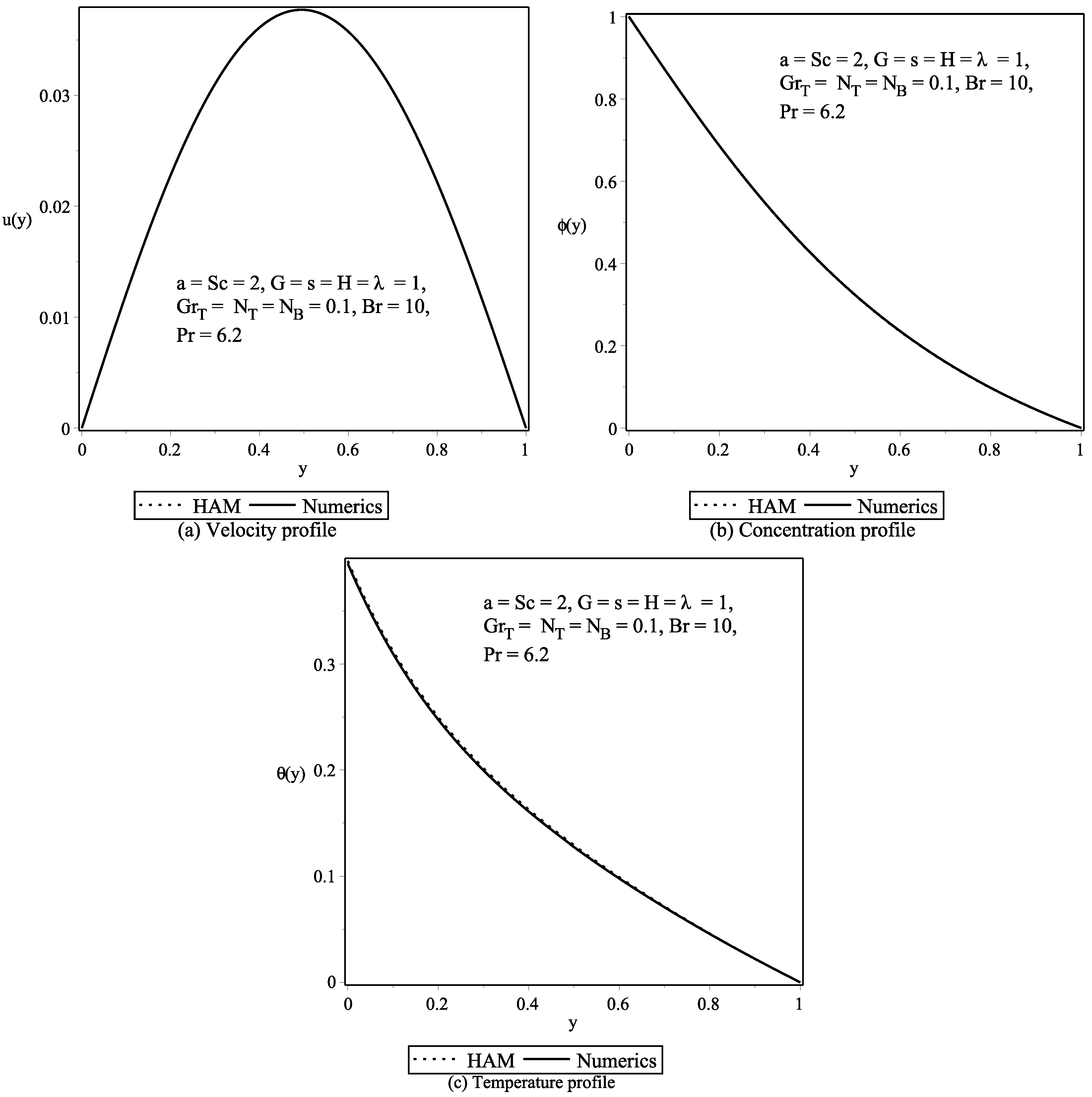
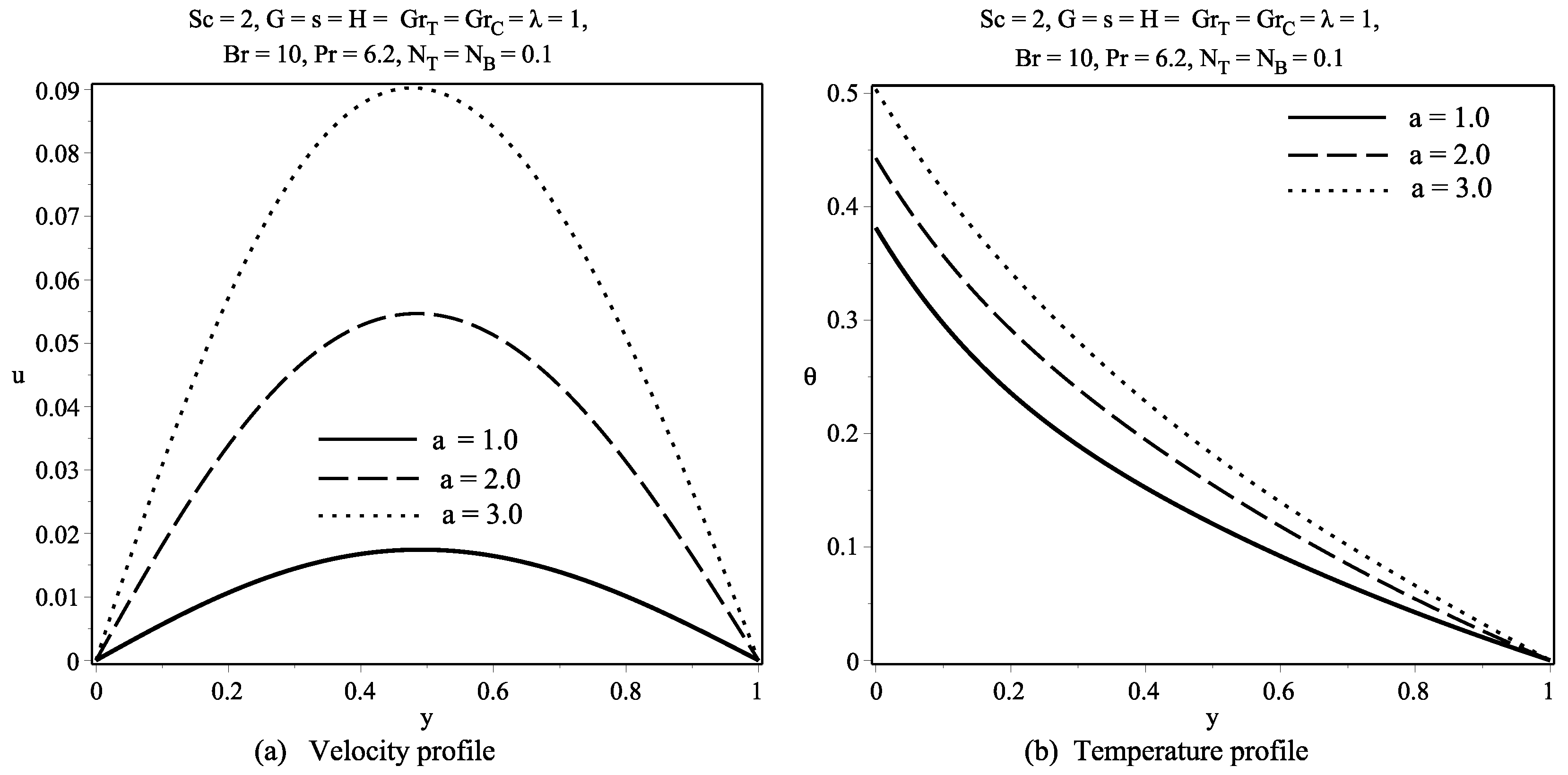
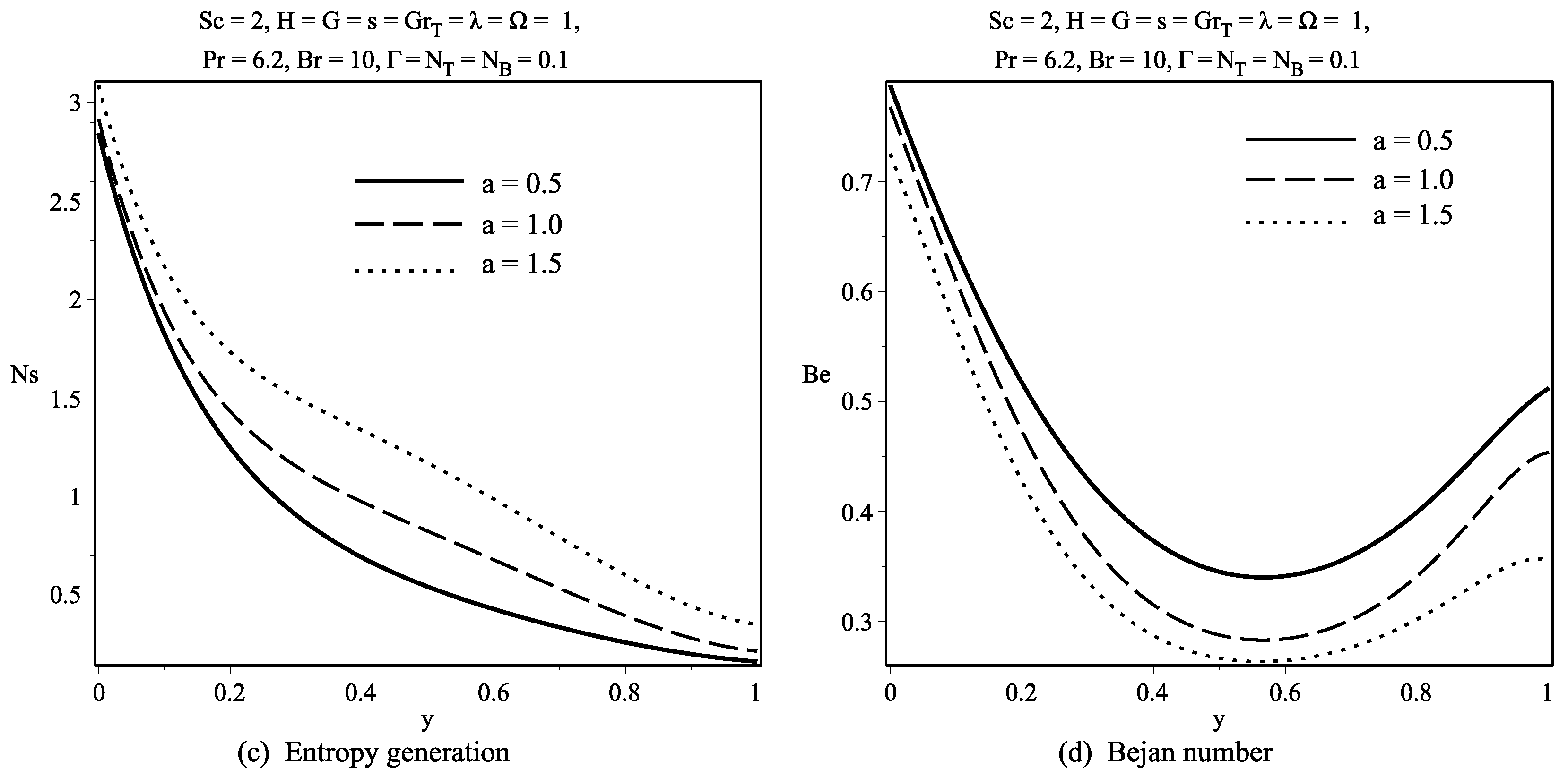
In Figure 3 the results obtained by using HAM are validated numerically by using the fourth–fifth order Runge–Kutta–Fehlberg method RK4; the result shows an excellent agreement in the three cases thus showing the strength of the method in handling coupled nonlinear problems. Evidently, the computation suggests the uniqueness of the solutions. Figure 4 demonstrates the effect of the couple stress inverse parameter on the flow profiles. As seen from the plot in Figure 4a, the couple stress inverse parameter is seen to elevate all the profiles except for the Bejan number. The physical reason is that, as the couple stress inverse parameter increases, the flow velocity increases due to shear thinning of the fluid. Therefore, it enhances the temperature too due to the increasing inter-molecular interactions as presented in Figure 4c. More so, as seen in Figure 4b, the rise in flow and temperature elevates the entropy generation in the porous channel across the channel width, and this decreases the heat transfer rate in the flow domain. Therefore, heat irreversibility due to frictional interaction and diffusion dominates over the heat transfer irreversibility in the flow channel as reported in Figure 4d. In the real sense, the reverse phenomenon is experienced as the couple stress inverse parameter increases.
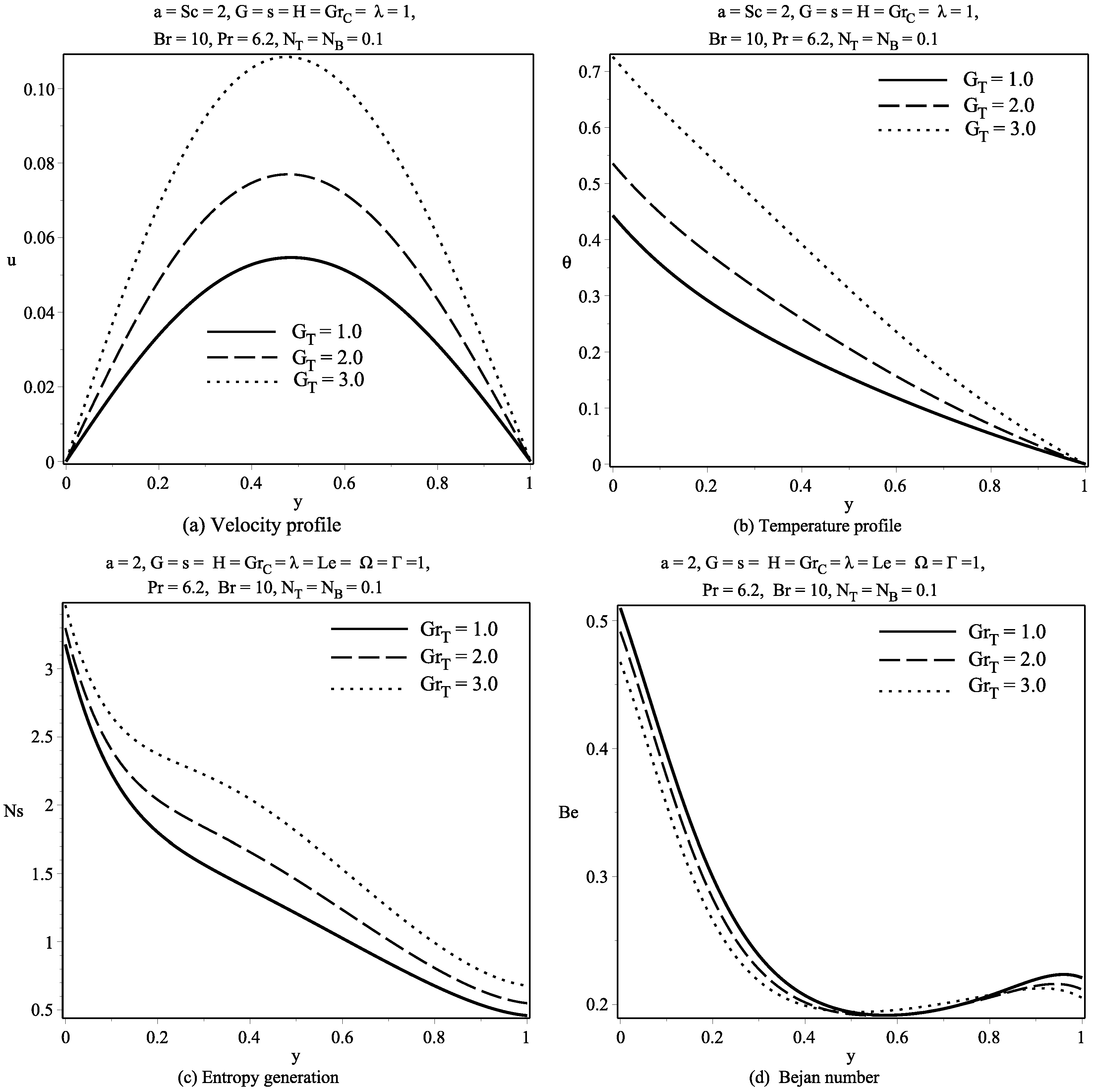
Figure 5 depicts the response of the variation in Brinkman number to the flow profiles. In Figure 5a, an increase in Brinkman number is observed to enhance the fluid flow velocity. This is true since increasing the value of Brinkman number leads to a rise in the heat transfer rate from the channel wall to the couple stress nanofluid within the flow channel. As a result, there is a rise in the kinetic energy of the fluid particles in the core region of the channel. Thus, an increase in Brinkman number is seen to improve the fluid temperature of the fluid particles closer to the heat flux region due to external heating of the channel wall as shown in Figure 5c. The combined effect of the enhance flow and heat transfer is seen to elevate the entropy generation rate in the flow channel in Figure 5b and decreases the heat transfer irreversibility. As a result, the diffusive and frictional heat irreversibility dominates over the transfer irreversibility as presented in Figure 5d. In Figure 6, the effects of the thermal Grashof number on the overall structure is presented. As the temperature of the fluid rises, the volumetric thermal expansion increases. This enhances the fluid flow velocity (see Figure 6a) since the density of the fluid decreases. The inter-molecular bonds maintaining the fluid particles weaken with increasing thermal Grashof number, and therefore, the fluid temperature increases due to increased inter-particle collision as seen in Figure 6c. Entropy generation, therefore, rises due to irreversible heat flow, the destructive nature of the chemical reaction thus leading to the dominance of thermal irreversibility due to frictional forces and diffusion over irreversibility due to heat transfer as observed in Figure 6b,d, respectively. Similar behaviour is experienced as the solutal Grashof number increases in Figure 7.
Figure 8a shows the interaction of couple stress nanofluid particles with the external magnetic field imposed across the flow channel. As seen in the plot provided in Figure 8a, as the magnetic field intensity parameter increases, the flow velocity declines due to particle agglomeration and the retarding action of the Lorentz forces as the Hartman number increases. As a result, the fluid temperature decreases as seen in Figure 8c. The decrease in the flow and temperature profiles led to decline in the entropy generation within the flow channel as shown in Figure 8b. This means that irreversibility due to fluid friction will be higher than the diffusive and heat transfer irreversibility as shown in Figure 8d.
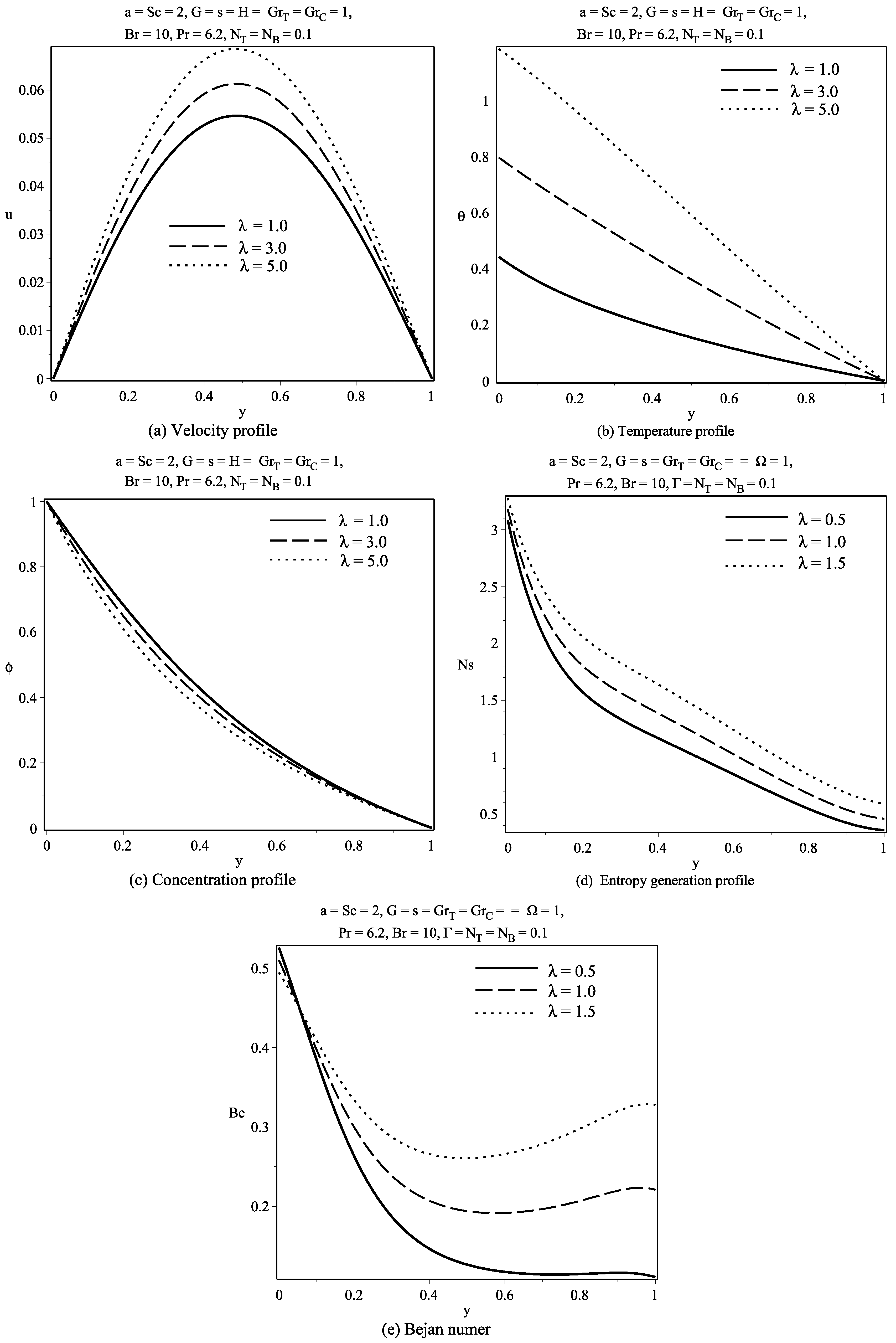
In Figure 9, the effects of a constant heat source on the velocity and temperature profiles are illustrated. From the result in Figure 9a, an increase in the heat source parameter is seen to enhance the flow velocity due to shear thinning property associated with decreased fluid viscosity as the temperature rises. However, as the couple stress fluid is heated, it expands with increased buoyancy-force and the fluid temperature increases as seen in Figure 9c. In Figure 9b, an increase in the heat source parameter is observed to decrease the fluid concentration profile. This is physically correct due to the destructive nature of the chemical reaction. As a result, the entropy generation rises across the flow channel as seen in Figure 9d and heat irreversibility dominates the Bejan number as reported in Figure 9e.
Figure 10 represents the effect of Schmidt number on the flow profiles. As seen in Figure 10a, an increase in Schmidt number is seen to decrease the fluid flow velocity. This is because of the increased viscous force within the flowing fluid layers. This leads to reduced fluid temperature since fluid particle collision is discouraged as seen in Figure 10c. Moreover, an increase in Schmidt number is seen to decrease the concentration of the reacting species due to reduced diffusive force in the couple stress nanofluid. The net balance is noted in Figure 10b. In Figure 10d, entropy generation is seen to be higher in the region subjected to constant heat flux while it declines at the other part of the channel. Subsequently, this resulted in minimal heat transfer irreversibility in the area exposed to heat flux while it dominates over both the diffusive and frictional irreversibility at the other part of the channel as presented in Figure 10e.
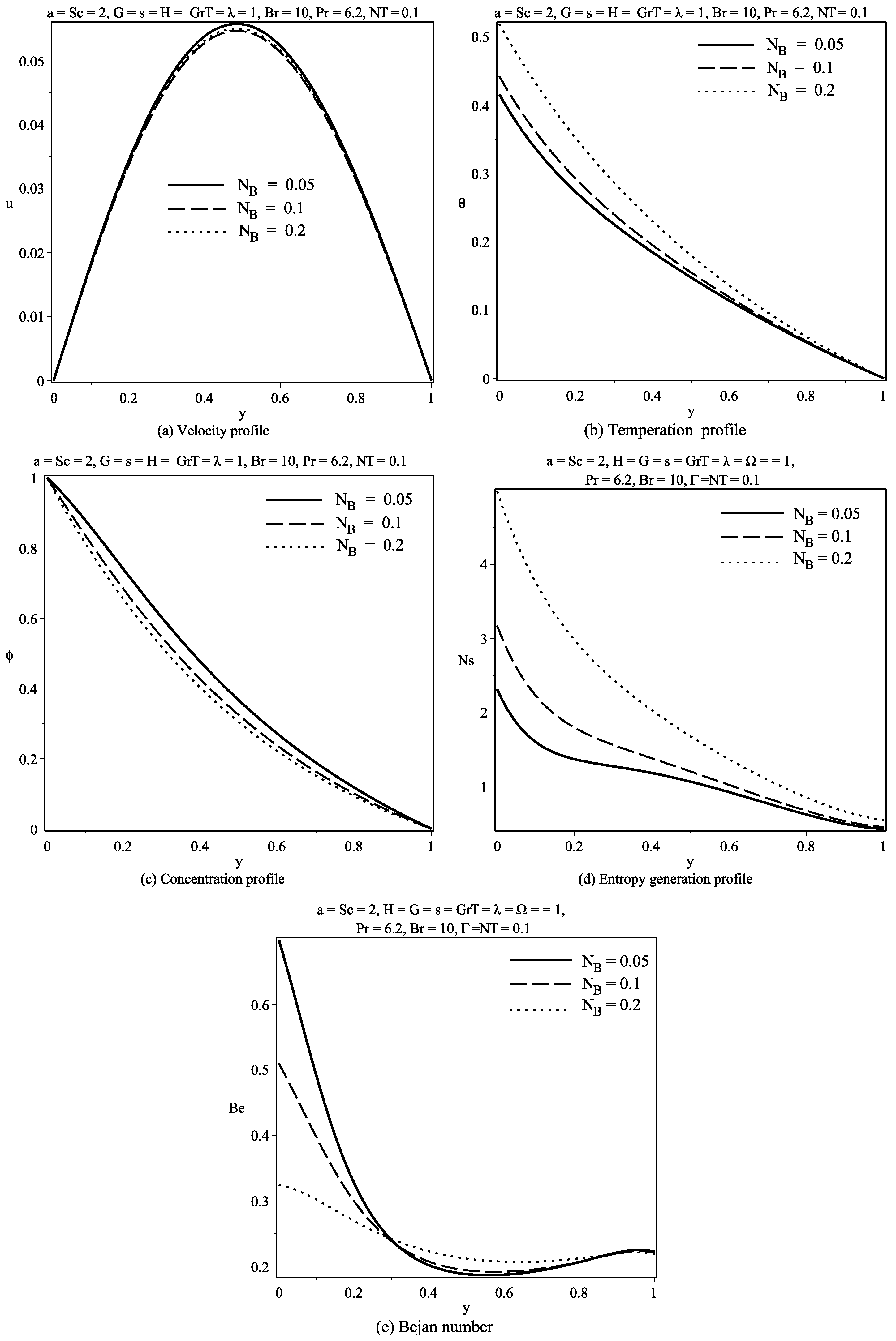
Figure 11 represents the variations of the dimensionless Brownian motion coefficient. From the random motion it is seen to distort the laminar motion of the fluid particles as seen in Figure 11a while it enhances the fluid inter-particle collision. As a result, the fluid temperature rises as seen in Figure 11b. By increasing the randomized motion coefficient, the chemical reaction profile is decreased due to destructive nature of the reaction. This elevates the entropy generated in the flow region as reported in Figure 11d and heat irreversibility due to diffusion dominates at the suction wall only, but in the core area, heat transfer irreversibility dominates over the frictional and diffusive irreversibility.
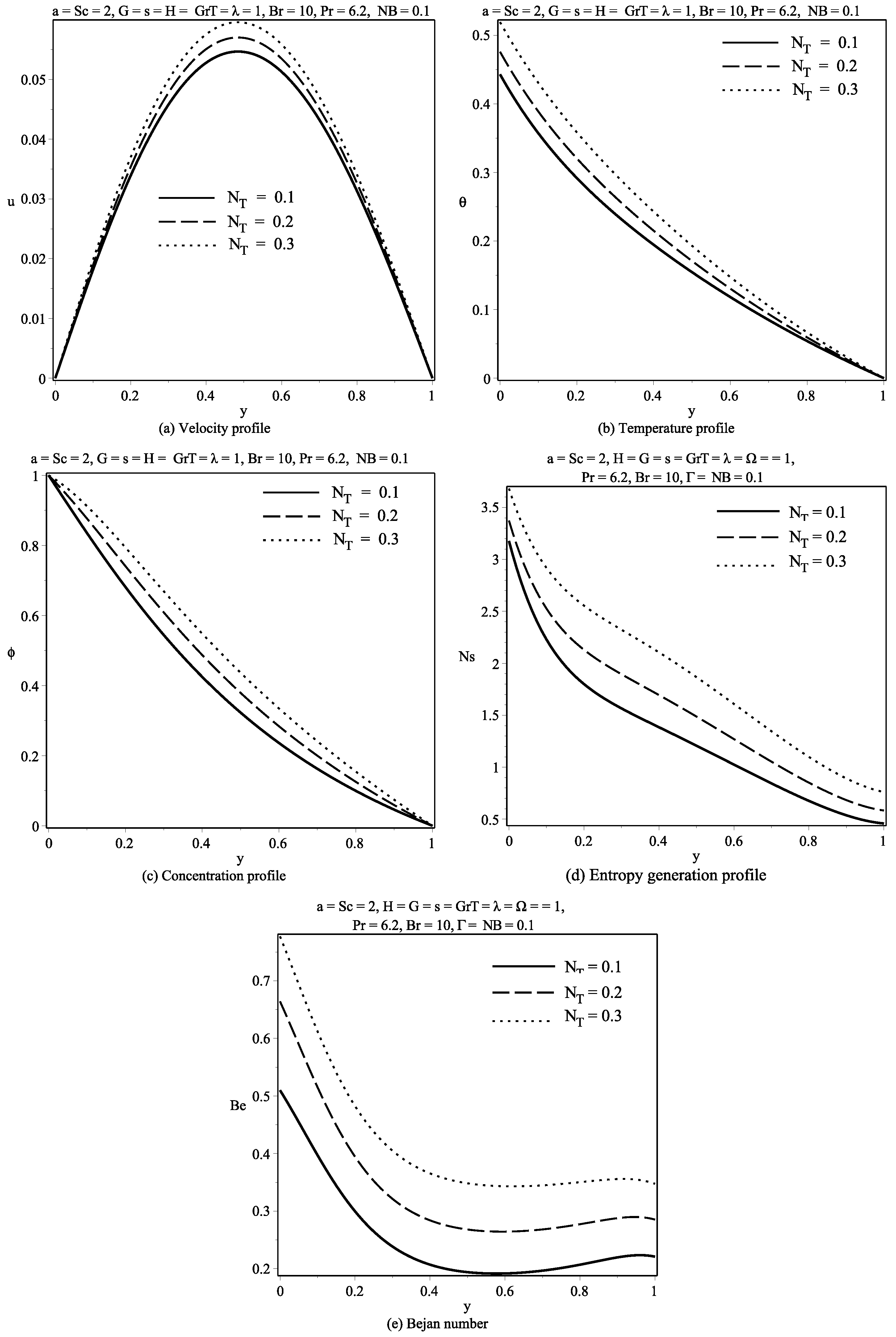
As the thermophoresis parameter increases, there is a rise in fluid velocity as shown in Figure 12a. In Figure 12b, as the thermophoresis parameter increases, there is an increase in the fluid temperature due to increased temperature gradient since heated fluid particles tend to migrate from the hot region of the channel to cold area as seen in Figure 12b. This further elevates the concentration profile as displayed in Figure 12c. Evidently, the entropy generated within the region is expected to rise as reported in Figure 12d. Finally, Figure 12e, heat transfer irreversibility is expected to dominate over irreversibility from viscous dissipation and diffusion.
7. Conclusions
In this work, the flow and heat transfer in a magnetohydrodynamic Cu–water couple stress nanofluid through a vertical channel subjected to constant heat flux has been studied. The equations governing the fluid flow are formulated, non-dimensionalized, and solved using the homotopy analysis method and are validated numerically. These solutions were shown to be convergent and were used to compute the entropy and Bejan profiles. The major contribution to knowledge is that, for adequate energy conservation and management, parameters leading to increase entropy generation in the flow channel need to be minimized for optimal performance of the thermo-fluid set up.
Author Contributions
All authors contributed equally to this work.
Conflicts of Interest
The authors declare no conflict of interest.
References
- Choi, S. Enhancing Thermal Conductivity of Fluids With Nanoparticles in Developments and Applications of Non-Newtonian Flows. ASME 1995, 66, 99–105. [Google Scholar]
- Sheikholeslami, M.; Ashorynejad, H.R.; Domairry, G.; Hashim, I. Flow and Heat Transfer of Cu-Water Nanofluid between a Stretching Sheet and a Porous Surface in a Rotating System. J. Appl. Math. 2012, 18. [Google Scholar] [CrossRef]
- Sheikholeslami, M.; Gorji Bandpy, M.; Ellahi, R.; Hassan, M.; Soleimani, S. Effects of MHD on Cu-water nanofluid flow and heat transfer by means of CVFEM. J. Magn. Magn. Mater. 2014, 349, 188–200. [Google Scholar] [CrossRef]
- Das, K. Cu-water nanofluid flow and heat transfer over a shrinking sheet. J. Mech. Sci. Technol. 2014, 28, 5089–5094. [Google Scholar] [CrossRef]
- Heris, S.Z.; Etemad, S.G.; Esfahany, M.N. Convective Heat Transfer of a Cu/Water Nanofluid Flowing Through a Circular Tube. Exp. Heat Transf. 2009, 22, 217–227. [Google Scholar] [CrossRef]
- Sheikholeslami, M.; Ganji, D.D. Heat transfer of Cu-water nanofluid flow between parallel plates. Powder Technol. 2013, 235, 873–879. [Google Scholar] [CrossRef]
- Domairry, G.; Hatami, M. Squeezing Cu-water nanofluid flow analysis between parallel plates by DTM-Pad Method. J. Mol. Liq. 2014, 193, 37–44. [Google Scholar] [CrossRef]
- Das, K.; Duari, P.R.; Kumar, P.K. Solar Radiation Effects on Cu-Water Nanofluid Flow over a Stretching Sheet with Surface Slip and Temperature Jump. Arab. J. Sci. Eng. 2014, 39, 9015–9023. [Google Scholar] [CrossRef]
- Hayat, T.; Rashid, M.; Imtiaz, M.; Alsaedi, A. Magnetohydrodynamic (MHD) flow of Cu-water nanofluid due to a rotating disk with partial slip. AIP Adv. 2015. [Google Scholar] [CrossRef]
- Akbar, N.S.; Nadeem, S. Intestinal Flow of a Couple Stress Nanofluid in Arteries. IEEE Trans. NanoBiosci. 2013, 12, 332–339. [Google Scholar] [CrossRef] [PubMed]
- Rehman, A.; Nadeem, S.; Malik, M.Y. Stagnation flow of couple stress nanofluid over an exponentially stretching sheet through a porous medium. J. Power Technol. 2013, 93, 122–132. [Google Scholar]
- Awais, M.; Saleem, S.; Hayat, T.; Irum, S. Hydromagnetic couple-stress nanofluid flow over a moving convective wall: OHAM analysis. Acta Astronaut. 2016, 129, 271–276. [Google Scholar] [CrossRef]
- Hayat, T.; Muhammad, T.; Alsaedi, A.; Alhuthali, M.S. Magnetohydrodynamic three-dimensional flow of viscoelastic nanofluid in the presence of nonlinear thermal radiation. J. Magn. Magn. Mater. 2015, 385, 222–229. [Google Scholar] [CrossRef]
- Hayat, T.; Sajjad, R.; Alsaedi, A.; Muhammad, T.; Ellahi, R. On squeezed flow of couple stress nanofluid between two parallel plates. Res. Phys. 2017, 7, 553–561. [Google Scholar] [CrossRef]
- Bejan, A. Entropy generation minimization: The new thermodynamics of finite size devices and finite time processes. J. Appl. Phys. 1996, 79. [Google Scholar] [CrossRef]
- Bejan, A. A study of entropy generation in fundamental convective heat transfer. J. Heat Transf. 1979, 101, 718–725. [Google Scholar] [CrossRef]
- Ibáñez, G.; López, A.; Pantoja, J.; Moreira, J. Entropy generation analysis of a nanofluid flow in MHD porous microchannel with hydrodynamic slip and thermal radiation. Int. J. Heat Mass Transf. 2016, 100, 89–97. [Google Scholar] [CrossRef]
- Hussain, S.; Mehmood, K.; Sagheer, M. MHD mixed convection and entropy generation of water–alumina nanofluid flow in a double lid driven cavity with discrete heating. J. Magn. Magn. Mater. 2016, 419, 140–155. [Google Scholar] [CrossRef]
- Selimefendigil, F.; Hakan, F.; Chamkha, A.J. MHD mixed convection and entropy generation of nanofluid filled lid driven cavity under the influence of inclined magnetic fields imposed to its upper and lower diagonal triangular domains. J. Magn. Magn. Mater. 2016, 406, 266–281. [Google Scholar] [CrossRef]
- Kefayati, G.H.R. Simulation of heat transfer and entropy generation of MHD natural convection of non-Newtonian nanofluid in an enclosure. Int. J. Heat Mass Transf. 2016, 92, 1066–1089. [Google Scholar] [CrossRef]
- Fersadou, I.; Kahalerras, H.; El Ganaoui, M. MHD mixed convection and entropy generation of a nanofluid in a vertical porous channel. Compt. Fld. 2015, 121, 164–179. [Google Scholar] [CrossRef]
- Abolbashari, A.H.; Freidoonimehr, N.; Nazari, F.; Rashidi, M.M. Entropy analysis for an unsteady MHD flow past a stretching permeable surface in nanofluid. Powder Technol. 2014, 267, 256–267. [Google Scholar] [CrossRef]
- Cho, C.-C. Influence of magnetic field on natural convection and entropy generation in Cu–waternanofluid-filled cavity with wavy surfaces. Int. J. Heat Mass Transf. 2016, 101, 637–647. [Google Scholar] [CrossRef]
- Chen, C.; Chen, B.; Liu, C. Entropy generation in mixed convection magnetohydrodynamic nanofluid flow in vertical channel. Int. J. Heat Mass Transf. 2015, 91, 1026–1033. [Google Scholar] [CrossRef]
- Sheikholeslami, M.; Ganji, D.D. Nanofluid hydrothermal behavior in existence of Lorentz forces considering Joule heating effect. J. Mol. Liq. 2016, 224, 526–537. [Google Scholar] [CrossRef]
- Mehrez, Z.; El Cafsi, A.; Belghith, A.; Patrick, L. MHD effects on heat transfer and entropy generation of nanofluid flow in an open cavity. J. Magn. Magn. Mater. 2015, 374, 214–224. [Google Scholar] [CrossRef]
- Rashidi, M.M.; Abelman, S.; Freidooni, N. Entropy generation in steady MHD flow due to a rotating porous disk in a nanofluid. Int. J. Heat Mass Transf. 2013, 62, 515–525. [Google Scholar] [CrossRef]
- Hajialigol, N.; Fattahi, A.; Ahmadi, M.H.; Qomi, M.E.; Kakoli, E. MHD mixed convection and entropy generation in a 3-D microchannel using Al2O3–water, nanofluid. J. Taiwan Inst. Chem. Eng. 2015, 46, 30–42. [Google Scholar] [CrossRef]
- Mahmoudi, A.H.; Pop, I.; Shahi, M.; Talebi, F. MHD natural convection and entropy generation in a trapezoidal enclosure using Cu–water nanofluid. Comput. Fluds 2013, 72, 46–62. [Google Scholar] [CrossRef]
- Uddin, M.J.; Anwar Bég, O.; Amin, N.S. Hydromagnetic transport phenomena from a stretching or shrinking nonlinear nanomaterial sheet with Navier slip and convective heating: A model for bio-nano-materials processing. J. Magn. Magn. Mater. 2014, 368, 252–261. [Google Scholar] [CrossRef]
- Khalili, S.; Tamim, H.; Khalili, A.; Rashidi, M.M. Unsteady convective heat and mass transfer in pseudoplastic nanofluid over a stretching wall. Adv. Powder Technol. 2015, 26, 1319–1326. [Google Scholar] [CrossRef]
- Mabood, F.; Shateyi, S.; Momoniat, E.; Freidoonimehr, N. MHD stagnation point flow heat and mass transfer of nanofluids in porous medium with radiation, viscous dissipation and chemical reaction. Adv. Powder Technol. 2016, 27, 724–749. [Google Scholar] [CrossRef]
- Khan, S.T.; Al-Khedhairy, A.A. ZnO and TiO2 nanoparticles as novel antimicrobial agents for oral hygiene: A review. J. Nanopart. Res. 2015, 17, 276. [Google Scholar] [CrossRef]
- Kherbeet, A.S.; Mohammed, H.A.; Salman, B.H.; Ahmed, H.E.; Alawi, O.A.; Rashidi, M.M. Experimental Study of Nanofluid Flow and Heat Transfer over Microscale Backward and Forward Facing Steps. Exp. Therm. Fluid Sci. 2015. [Google Scholar] [CrossRef]
- Liao, S.J. Beyond Perturbation: Introduction to the Homotopy Analysis Method; CRC Press: Boca Raton, FL, USA; Chapman and Hall: London, UK, 2003. [Google Scholar]
- Liao, S.J. Homotopy Analysis Method in Nonlinear Differential Equations; Higher Education Press: Beijing, China; Springer: Berlin/Heidelberg, Germany, 2012. [Google Scholar]
Figure 1.
Physical model of the problem.
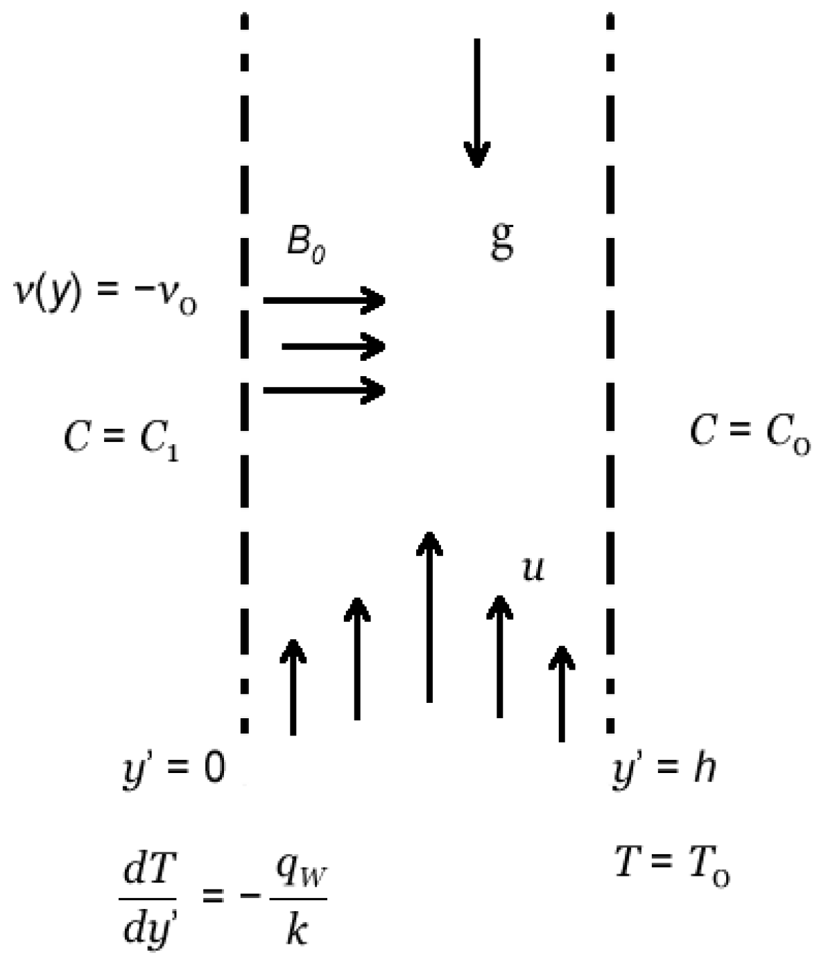
Figure 2.
Variations of convergence parameters in the solutions.
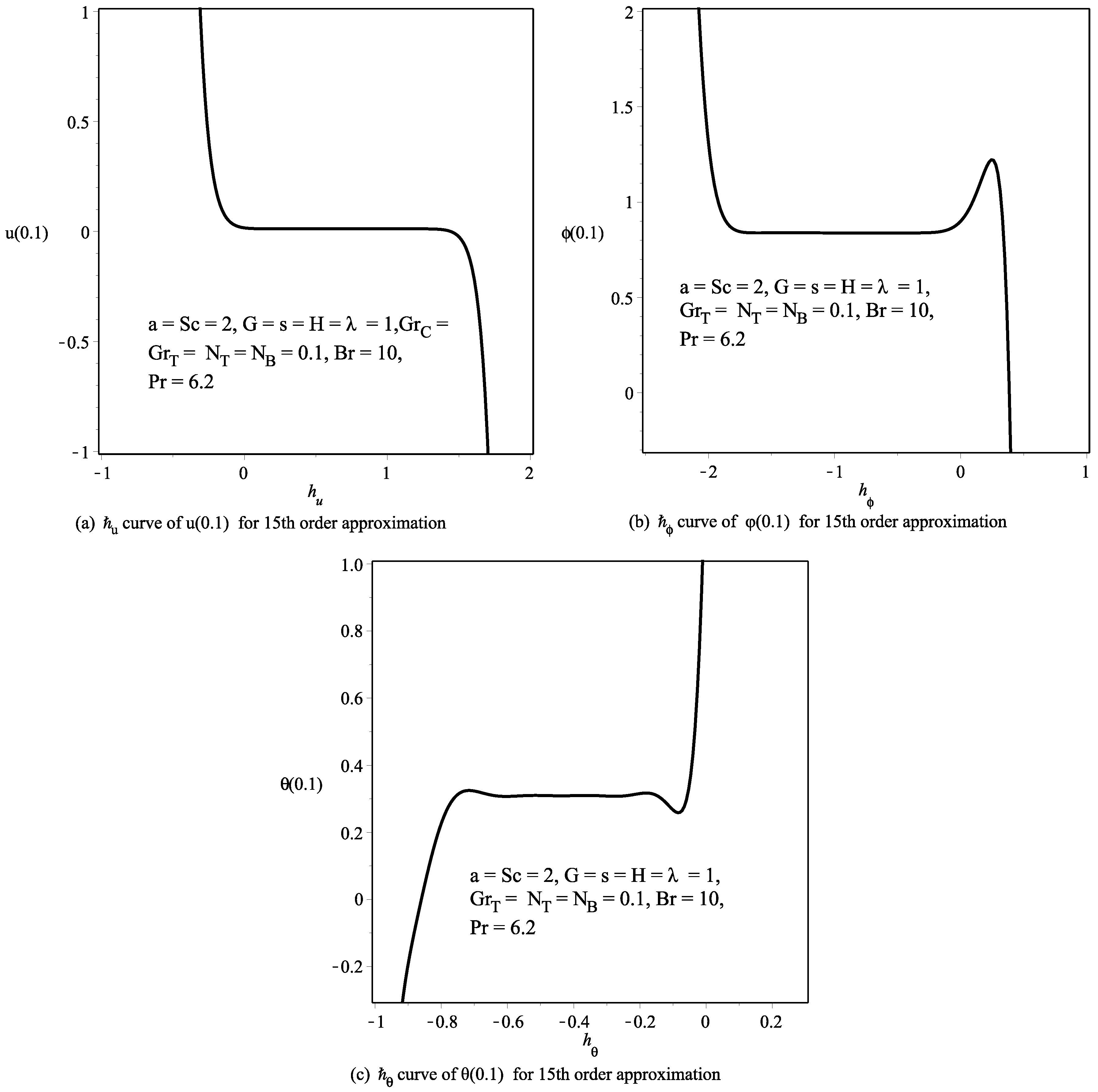
Figure 3.
Validation of solutions.

Figure 4.
Influence of couple stress inverse parameters.


Figure 5.
Influence of the Brinkman number.
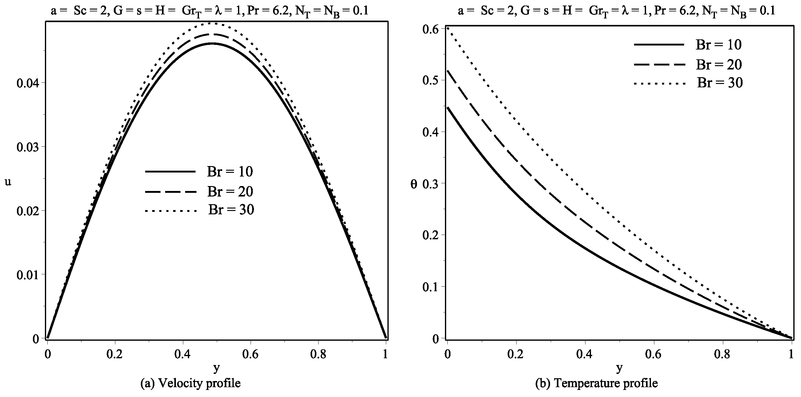

Figure 6.
Influence of the thermal Grashof number.

Figure 7.
Effects of the solutal Grashof number.
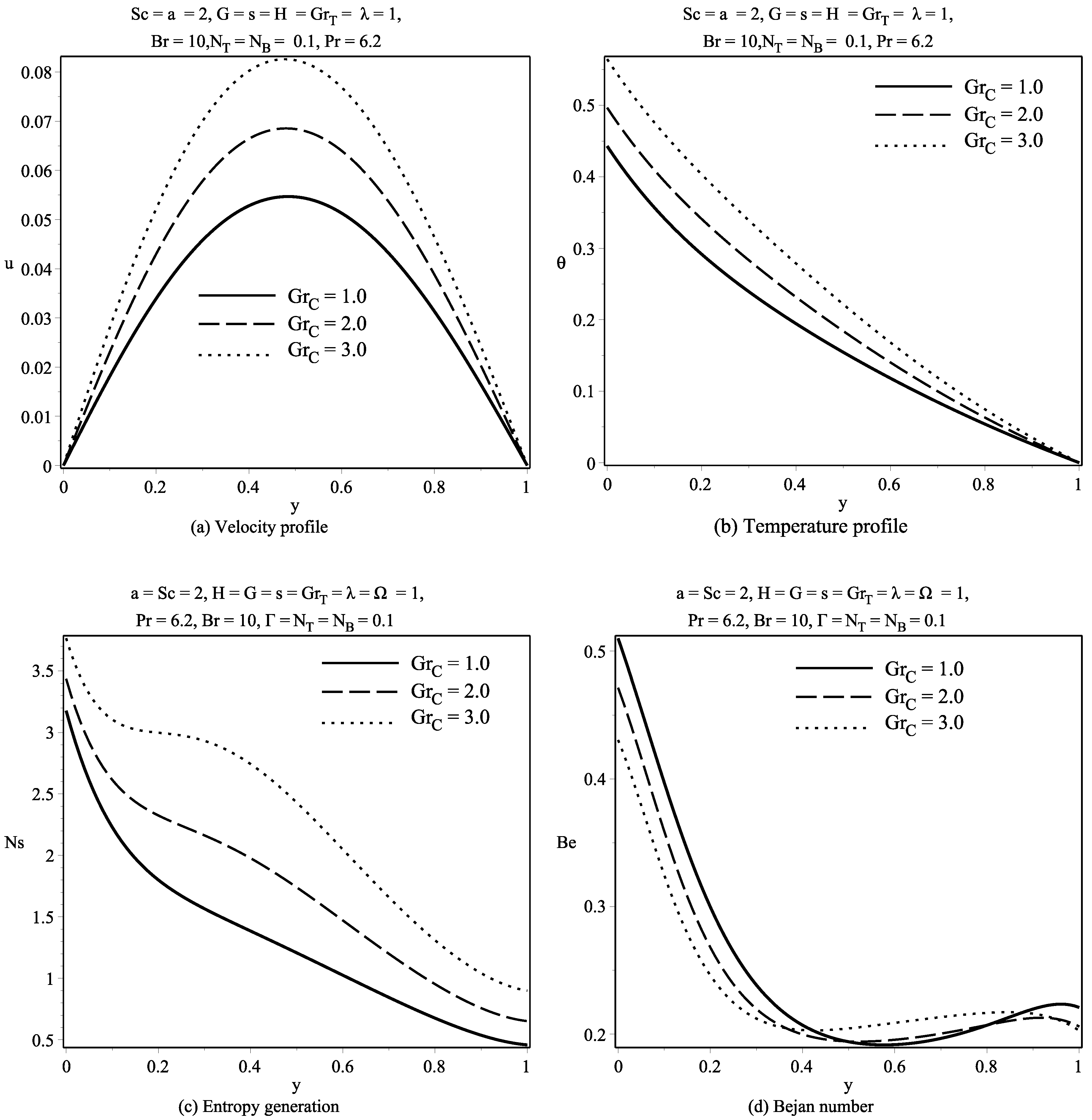
Figure 8.
Effects of the Hartmann number.
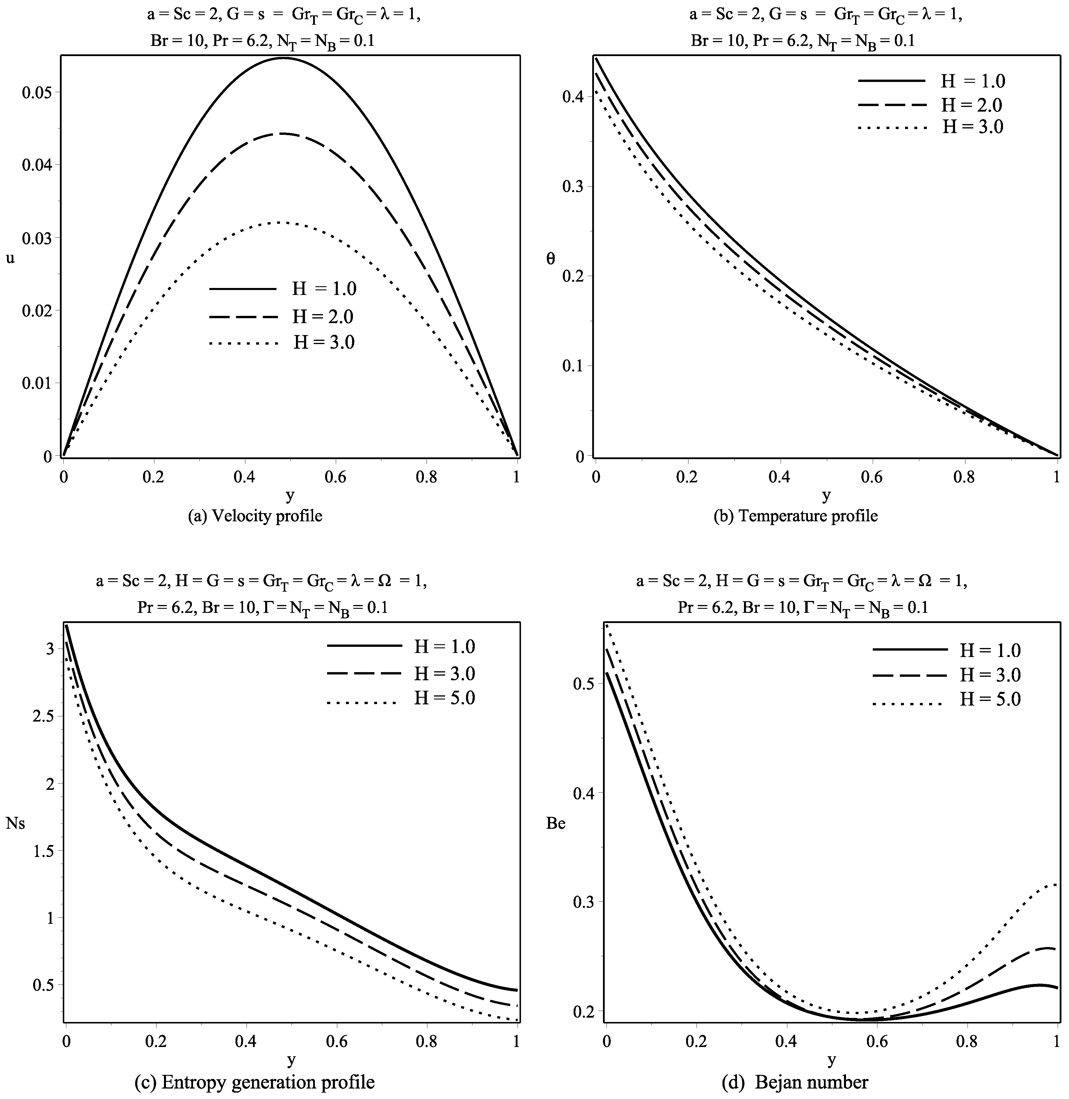
Figure 9.
Effects of constant heat source parameters.

Figure 10.
Effects of the Schmidt number.

Figure 11.
Effects of the Brownian motion parameter.

Figure 12.
Thermophoresis effect.


Table 1.
a = Sc = 2, G = H = s = , , Pr = 6.2, Br = 10, , .
| y | u HAM | u RK4 | Abs. Error | HAM | RK4 | Abs. Error |
|---|---|---|---|---|---|---|
| 0 | 0.00000 | 0.00000 | 0.000 | 0.39475 | 0.39473 | 1.6129 × |
| 0.1 | 0.01212 | 0.01212 | 3.952 × | 0.30974 | 0.30972 | 2.0124 × |
| 0.2 | 0.02282 | 0.02282 | 7.308 × | 0.24748 | 0.24746 | 2.1147 × |
| 0.3 | 0.03104 | 0.03104 | 9.892 × | 0.19967 | 0.19965 | 2.8675 × |
| 0.4 | 0.03612 | 0.03612 | 1.155 × | 0.16087 | 0.16082 | 4.7640 × |
| 0.5 | 0.03772 | 0.03772 | 1.236 × | 0.12763 | 0.12758 | 3.2397 × |
| 0.6 | 0.03575 | 0.03575 | 1.246 × | 0.09787 | 0.09795 | 7.9192 × |
| 0.7 | 0.03042 | 0.03042 | 1.222 × | 0.07056 | 0.07083 | 2.7514 × |
| 0.8 | 0.02218 | 0.02218 | 1.174 × | 0.04524 | 0.04565 | 4.1654 × |
| 0.9 | 0.01171 | 0.01171 | 1.092 × | 0.02180 | 0.02212 | 3.2119 × |
| 1.0 | 0.00000 | 0.00000 | 9.20 × | 0.00000 | 0.00000 | 2.0000 × |
Table 2.
a = Sc = 2, G = H = s = , , Pr = 6.2, Br = 10, , .
| y | HAM | RK4 | Abs. Error |
|---|---|---|---|
| 0 | 1.0000000 | 1.0000000 | 0.0000000 |
| 0.1 | 0.8387730 | 0. 8387837 | 1.07275 × |
| 0.2 | 0.6862309 | 0.6863211 | 9.01931 × |
| 0.3 | 0.5483278 | 0.5484970 | 1.6923 × |
| 0.4 | 0.4273287 | 0.4275787 | 2.5002 × |
| 0.5 | 0.3231850 | 0.3235501 | 3.65135 × |
| 0.6 | 0.2346430 | 0.2351325 | 4.84783 × |
| 0.7 | 0.1599510 | 0.16044790 | 5.280647 × |
| 0.8 | 0.0972060 | 0.0976057 | 3.99661 × |
| 0.9 | 0.0444898 | 0.0446433 | 1.534344 × |
| 1.0 | 0.0000000 | 0.000000 | 0.00000000 |
© 2017 by the authors. Licensee MDPI, Basel, Switzerland. This article is an open access article distributed under the terms and conditions of the Creative Commons Attribution (CC BY) license (http://creativecommons.org/licenses/by/4.0/).
Share and Cite
MDPI and ACS Style
Adesanya, S.O.; Ogunseye, H.A.; Falade, J.A.; Lebelo, R.S. Thermodynamic Analysis for Buoyancy-Induced Couple Stress Nanofluid Flow with Constant Heat Flux. Entropy 2017, 19, 580. https://doi.org/10.3390/e19110580
AMA Style
Adesanya SO, Ogunseye HA, Falade JA, Lebelo RS. Thermodynamic Analysis for Buoyancy-Induced Couple Stress Nanofluid Flow with Constant Heat Flux. Entropy. 2017; 19(11):580. https://doi.org/10.3390/e19110580
Chicago/Turabian StyleAdesanya, Samuel O., Hammed A. Ogunseye, J. A. Falade, and R.S. Lebelo. 2017. "Thermodynamic Analysis for Buoyancy-Induced Couple Stress Nanofluid Flow with Constant Heat Flux" Entropy 19, no. 11: 580. https://doi.org/10.3390/e19110580
Note that from the first issue of 2016, this journal uses article numbers instead of page numbers. See further details here.