Entropy Production in Stochastics


Department of Water Resources, School of Civil Engineeringh, National Technical University of Athens, 15780 Athina, Greece
Entropy 2017, 19(11), 581; https://doi.org/10.3390/e19110581
Submission received: 14 September 2017
/
Revised: 21 October 2017
/
Accepted: 23 October 2017
/
Published: 30 October 2017
(This article belongs to the Special Issue Entropy Applications in Environmental and Water Engineering)
Abstract
:While the modern definition of entropy is genuinely probabilistic, in entropy production the classical thermodynamic definition, as in heat transfer, is typically used. Here we explore the concept of entropy production within stochastics and, particularly, two forms of entropy production in logarithmic time, unconditionally (EPLT) or conditionally on the past and present having been observed (CEPLT). We study the theoretical properties of both forms, in general and in application to a broad set of stochastic processes. A main question investigated, related to model identification and fitting from data, is how to estimate the entropy production from a time series. It turns out that there is a link of the EPLT with the climacogram, and of the CEPLT with two additional tools introduced here, namely the differenced climacogram and the climacospectrum. In particular, EPLT and CEPLT are related to slopes of log-log plots of these tools, with the asymptotic slopes at the tails being most important as they justify the emergence of scaling laws of second-order characteristics of stochastic processes. As a real-world application, we use an extraordinary long time series of turbulent velocity and show how a parsimonious stochastic model can be identified and fitted using the tools developed.
1. Introduction
Entropy was first recognized as a probabilistic concept in 1887 by Boltzmann [1], who established a relationship of entropy with probabilities of statistical mechanical system states, thus explaining the Second Law of Thermodynamics as the tendency of the system to run toward more probable states. In 1948 Shannon [2] used an essentially similar, albeit more general, definition of entropy as a probabilistic concept, a measure of information or, equivalently, uncertainty. In 1957 Jaynes [3] introduced the principle of maximum entropy thus equipping the entropy concept with a powerful tool for logical inference.
A decade later, probabilistic entropy and the principle of maximum entropy were used in geophysical sciences and particularly hydrology, initially for parameter estimation of models [4] and probability distributions [5]. Detailed reviews on the use of entropy in applications in hydrology, and water and environmental engineering have been provided by Singh ([6,7] and more recently [8,9,10,11]). Most applications of probabilistic entropy are static, disregarding time. In studying systems out of the equilibrium, time should necessarily be involved (e.g., [12]) and the paths of the systems should be inferred. The more recently developed, within non-equilibrium thermodynamics, extremum principles of entropy production attempt to predict the most likely path of system evolution [13,14,15]. Central among the latter are Prigogine’s minimum entropy production principle [16] and Ziegler’s maximum entropy production principle [17,18].
Entropy production in thermodynamic systems is typically defined in terms of the derivative of entropy with respect to time, while the entropy flux in open systems is also considered. Niven and Ozawa [19] provide a general definition of entropy production along with a brief review of applications of extremum principles in geophysics and particularly hydrology. It can be seen that in these applications, the entropy concept is typically used with its classical thermodynamic definition and in deterministic terms, without reference to its modern probabilistic definition.
Deterministic descriptions of the evolution of uncertain physical and geophysical systems are generally inefficient [20,21], while a much more powerful alternative is offered by stochastics. The term ‘stochastics’ describes the mathematics of random variables and stochastic processes, and comprises probability theory, statistics and stochastic processes. While the entropy concept is well defined within stochastics, the entropy production does not have a scientifically mature definition. By analogy to classical thermodynamic versions, we may define entropy production in stochastics as the derivative of (probabilistic) entropy with respect to time. As here we deal with a single stochastic process and not with interaction of many processes, there are no entropy fluxes and, thus, entropy production should merely rely on the time derivative of entropy. In an earlier study [22], the derivative with respect to the logarithm of time was introduced and termed ‘entropy production in logarithmic time’ (EPLT). Differentiation with respect to the logarithm of time has some attractive elements, such as:
- It is dimensionless as d(ln t) = dt/t and thus, given that entropy is a dimensionless quantity per se (see next section), the EPLT remains a dimensionless quantity.
- It is consistent with the notion of the ‘arrow of time’. Usually entropy per se is related to the time asymmetry and the Second Law is regarded as the origin of the arrow. However, it may be simpler to think that it is the action of observation that creates time asymmetry. In this respect, we can set t = 0 for the observation time, i.e., the present, while t < 0 denotes the observable past and t > 0 denotes the unknown future. The fact that the past is observable, but the future not, generates the asymmetry. It is clarified that when the future becomes observable, it is no longer future; rather it has become present or past. Once the future (t > 0) is treated separately from the past, it is legitimate to differentiate with respect to the logarithm of time.
- It makes extremization of entropy production easier, particularly for asymptotic times t → 0 and t → ∞, as it avoids infinite or zero values of entropy production [22]; indeed, the asymptotic values of EPLT are always bounded (see Section 2.4).
- It provides the means to study or even explain the scaling behaviour often observed in geophysical processes (see Section 2.2 and Section 2.4).
Here we advance the study of the EPLT concept, with particular emphasis on the conditional entropy production (CEPLT), when the past and present have been observed (Section 2.2). The theoretical properties of EPLT and CEPLT are studied in a general setting and in application to a broad set of specific types of stochastic processes (Section 3.1 and Section 3.2). A main question studied is how the entropy production can be estimated from time series, i.e., realizations of stochastic processes. It turns out that there is a strong link of the EPLT with the climacogram, with the slope of a log-log plot of the latter representing the EPLT. Further, we introduce two new tools, additional to the climacogram and based on it, the differenced climacogram and the climacospectrum, where the latter has properties similar to those of the power spectrum. The slope of a log-log plot of either of the two additional tools can be used as an estimator of CEPLT. Of particular importance are the asymptotic slopes for time scale tending to zero or infinity (Section 3.3). To illustrate the theoretical and empirical properties of EPLT and CEPLT using real-world data and to test the applicability of the specific models proposed, a long time series of very fine resolution is needed in order to allow viewing the real-world behaviour at the far-left and the far-right tails. Fine resolution measurements of turbulence can provide an ideal test series and indeed a time series of length 36 × 106 of turbulent velocities is utilized for illustration and testing (Section 3.4).
To avoid bothering the reader with derivations and theoretical details, most of them have been put in a series of annexed sections organized as Appendix A.1. In addition, the details of the specific stochastic models and their behaviour have been grouped in Appendix A.2. While the two appendices are made in a stand-alone form separate from the body of the article, they are perhaps the most essential part of the study.
2. Methods
2.1. General Context
The evolution of a system state x over time t is usually represented as a trajectory x(t), but such a description is often inefficient. Instead, the evolution can be represented as a stochastic process x(t), which is a collection of (infinitely many) random variables x indexed by t. A realization (sample) x(t) of x(t) is a trajectory; if it is known at certain points ti, i = 1, 2, …, the realization is called a time series.
A random variable x is an abstract mathematical entity associated with a probability density (or mass) function f(x); the realizations x of x belong to a set of possible numerical values. Notice the different notation of random variables and hence stochastic processes (underlined, according to the Dutch notation [23]) from regular ones.
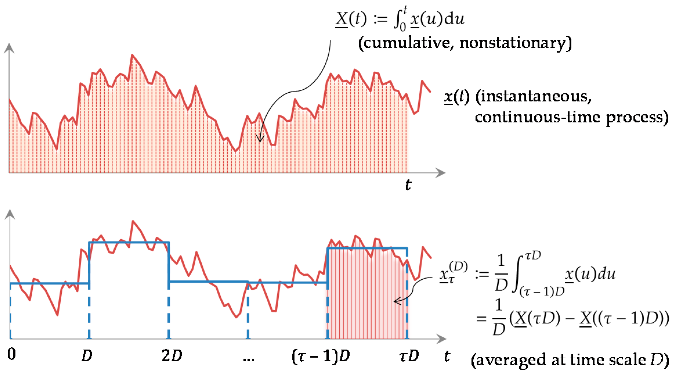
Most natural processes evolve in continuous time but they are observed in discrete time, typically by averaging. Accordingly, the stochastic processes devised to represent the natural processes should evolve in continuous time and be converted into discrete time, as illustrated in Figure 1.
While a stochastic process denotes, by conception, change (process = a series of changes), there should be some properties that are unchanged in time. This implies the concept of stationarity [25], which is central in stochastics. According to Kolmogorov’s definition [26], a stochastic process x(t) is stationary if the distributions of and coincide for any . By negation, in a nonstationary process the probability density for some (or all) τ is not equal to , which means that the mathematical expression of the latter should explicitly contain the time shift τ, or else that it should be a deterministic function of τ.
Stationarity is closely related to ergodicity, which in turn is a prerequisite to make inference from data, that is, induction. Within the stochastics domain ([20,27] (p. 427)) ergodicity is defined in the following manner: A stochastic process x(t) is ergodic if the time average of any function , as time tends to infinity, equals the true (ensemble) expectation . This allows the estimation (i.e., approximate calculation) of the true but unknown quantity (e.g., the true average ) from the available data, i.e., from the sample mean). Without stationarity there is no ergodicity and without ergodicity inference from data is impossible. More details about stationarity and ergodicity, and their importance, are provided by Koutsoyiannis and Montanari [25], along with highlights of the misconceptions and abuses of these concepts which abound in the literature.
For the remaining part of this article, unless otherwise stated, the processes are assumed to be stationary and ergodic, noting that nonstationary processes should be converted to stationary before their study. For example, the cumulative process X(t) in Figure 1 is nonstationary, but by differentiating it in time we obtain the stationary process x(t).
Without loss of generality we assume that the mean of the process x(t) is zero (E[x(t)] = 0) and we denote its variance as:
Let:
be the variances of the cumulative and the averaged process, respectively (note that Γ(0) = 0 and γ(0) = γ0). While Γ(t), the variance of the nonstationary process X(t), is a function of t, γ(k) is the variance of the stationary process , i.e., and thus it is not a function of time τ. We call Γ(t) and γ(k), as functions of time t and time scale k, the cumulative climacogram and the climacogram of the process, respectively.
γ0 ≔ Var[x(t)]
Γ(t) ≔ Var[X(t)], γ(k) ≔ Var[(1/k)(X(t + k) − X(t))] = Γ(k)/k2
The climacogram is the second central moment of the process, as a function of time scale, and thus it is a second-order characteristic of the process. Other customary second order characteristics of a stationary process are the autocovariance function c(h), where h denotes time lag, the power spectrum s(w), where w denotes frequency, and the structure function v(h) (also known, for a stationary process, as the semivariogram or variogram). The latter has a direct analogy based on the climacogram, the climacostructure function ξ(k). Definitions and notation for these second order characteristics are contained in Table 1 for the continuous time domain and in Table 2 for the discrete time case. All of these functions are transformations of one another, as shown in Table 3.
The climacogram, like the autocovariance function, is a positive definite function (see proof in Appendix A.1.2) but of the time scale k, rather than the time lag h. It is not as popular as the other tools but it has several good properties due to its simplicity, close relationship to entropy (see below), and more stable behaviour, which is an advantage in model identification and fitting from data. In particular, when estimated from data, the climacogram behaves better than all other tools, which involve high bias and statistical variation [24,28].
The climacogram involves bias too, but this can be determined analytically and included in the estimation. Specifically, assuming that we have n observations of the averaged process , at scale k = κD, so that T = nk is the observation period (rounded off to an integer multiple of k), the standard statistical estimator of variance has expected value:
where θ is the bias correction coefficient, given by [22,24]:
It becomes clear from the above equations, which are valid for any process, that direct estimation of the variance for any time scale k, let alone that of the instantaneous process γ0, is not possible merely from the data. We need to know the ratio and thus we should assume a stochastic model which evidently influences the estimation of . Once the model is assumed and its parameters estimated based on the data, we can expand our calculations to estimate the variance for any time scale, including that of the instantaneous scale γ0.
2.2. Entropy and Entropy Production
Historically entropy was introduced in thermodynamics but its rigorous definition was given within probability theory. Thermodynamic and probabilistic entropy are regarded by many as different concepts having in common only their name. However, here we embrace the view that they are essentially the same thing, as has articulated elsewhere [29,30]. According to the latter interpretation, the mathematical description of thermodynamic systems could be produced by the probabilistic definition of entropy. As an example indicating how powerful this interpretation could be, the law of phase change transition of water (Clausius-Clapeyron equation) has been produced in [30], with impressive agreement with reality, by maximizing, in a formal probabilistic frame, the entropy, i.e., the total uncertainty about the state of a single molecule of water.
In this frame, entropy (often called Boltzmann-Gibbs-Shannon entropy to give credit to its pioneers and distinguish it from other forms of generalized entropies) is a dimensionless measure of uncertainty defined as follows:
- For a discrete random variable x with probability mass function Pj ≔ P{x = xj}, j = 1, …, w:
- For a continuous random variable z with probability density function f(z):where m(x) is the density of a background measure (usually Lebesgue, i.e., m(x) = 1, with dimensions [x−1]).
Entropy acquires its importance from the principle of maximum entropy [3], which postulates that the entropy of a random variable should be at maximum, under some conditions, formulated as constraints, which incorporate the information that is given about this variable. Its physical counterpart, the tendency of entropy to become maximal (Second Law of thermodynamics) is the driving force of natural change.
The definition of the entropy of a stochastic process directly follows that of a random variable. Thus, the entropy of the cumulative process X(t) with probability density function f(X; t) is a dimensionless quantity defined as:
In a stochastic process, which by definition involves time, it is natural to consider the change of entropy in time. Intuitively, for the stochastic process X(t) we can define entropy production as the time derivative, i.e., Φ′[X(t)] := dΦ[X(t)]/dt. This has dimensions of inverse time. Koutsoyiannis [22] defined the entropy production in logarithmic time (EPLT) as the derivative of entropy in logarithmic time:
and showed that it has some advantages over Φ’[x(t)] as described above.
φ(t) ≡ φ[X(t)] ≔ Φ’[X(t)] t ≡ dΦ[X(t)]/d(lnt)
Assuming that the background density is constant, m(Χ) ≡ m, and using simple constraints related to the preservation of the mean and variance, the principle of maximum entropy yields that the probability distribution of X will be Gaussian. For a Gaussian process the entropy depends on its variance Γ(t) and is:
Hence:
Φ[X(t)] = (1/2) ln(2πe Γ(t)/m2)
φ(t) = Γ’(t) t/2Γ(t) = 1+ γ’(t) t/2γ(t)
Because of the simplicity of the Gaussian case, we are basing further analyses on that assumption, noting that for large times, due to the Central Limit Theorem, the cumulative process X(t) will tend to Gaussian, even if for the smallest scales it deviates from Gaussian.
A question arises whether φ(t) is a totally abstract concept useful for theoretical analyses only or it can be related to data, and visualized or estimated from them. The reply is fortunate if, in addition, we consider another concept, the log-log derivative (LLD) of a function f(x), formally expressed by:
This is visualized as the (local) slope on the popular log-log plot (plot of log f(x) vs. log x). It is then seen that (37) can be written as:
In other words, EPLT is visualized and estimated by the slope of a log-log plot of the climacogram.
φ(t) = ½ Γ#(t) = 1 + ½ γ#(t)
The quantity φ(t) represents the entropy production when nothing is known (observed) about the process realization. More interesting is the conditional EPLT (CEPLT, φC(t)) when the past (t < 0) and the present (t = 0) are observed. In this case, instead of the unconditional variance Γ(t) we should use a variance ΓC(t) conditional on the past and present. It has been shown [22,24] that for a Markov process (see definition of the Markov process in Section 3.1 and its details in Appendix A.2.1), the conditional variance is:
We note that the difference γ(k) − γ(2k) is always nonnegative (this is shown in Appendix A.1.3, Equation (A21)) and thus it can indeed represent a (conditional) variance.
For a non-Markov process the following adaptation is necessary:
where ε is a constant, ensuring that as k → ∞, ; the rationale of this limit is that the information about the past and present will tend not to affect the far distant future. As shown in the Appendix A.1.4, its value is:
It is easily verified that for a Markov process in which (see Appendix A.2.1), ε = 2, while for a Hurst-Kolmogorov process (original or filtered; see details in [24], in next session and in Appendix A.2) for which , , where H is the Hurst parameter.
Due to its mathematical form, we will refer to as the differenced climacogram. The inverse transformation, i.e., that giving the climacogram once the differenced climacogram is known, can be easily deduced by iterative evaluations also observing that (this is a necessary condition in order for a stochastic process to be ergodic [27] (p. 429)) and takes both the following forms:
whereas for numerical evaluations it should be kept in mind that for large time scales k, . Note that (43) entails:
and this is valid for any k. The importance of the differenced climacogram stems from the fact that it is directly related to the CEPLT, through its obvious relationship (similar to (39)):
As the differenced climacogram can be easily visualized from data, because it only needs calculation of variances, it directly provides a means for estimation and visualization of the CEPLT in terms of the slope in a log-log plot of the differenced climacogram.
In Appendix A.1.5 it is shown that the asymptotic properties of are:
In other words, we need both the climacogram γ(k) and the climacostructure function ξ(k) to express the asymptotic behaviour of . Once this is known, the asymptotic behaviour of CEPLT is also known from (45).
As shown in Appendix A.1.6, the differenced climacogram for persistent processes (see their definition in next subsection) is not integrable in (0, ∞). However, by slightly changing it multiplying with k, we can obtain an additional tool which is integrable and has some additional good properties. Specifically, we introduce the following tool, which, as we will see next, resembles the power spectrum and thus we refer to it as the climacospectrum:
The climacospectrum is also written in an alternative manner in terms of frequency w = 1/k:
The inverse transformation, i.e., that giving the climacogram once the climacospectrum is known, can be easily deduced with the same method as before, and takes the form:
A very good approximation in which the sum is replaced by an integral, is:
This holds for all k and its details are given in Appendix A.1.7. For small k, it is easy to see that the multiplier of the integral I(k) is 1. It follows that for small time scales k or large frequencies w = 1/k the climacospectrum, expressed in terms of frequency, has an area I(k) on the left of w equal to the variance γ(1/w). As shown in Appendix A.1.6, the entire area under the curve (i.e., I(0)) is precisely equal to the variance γ(0) of the instantaneous process, a property also shared by the power spectrum s(w). This is not the only connection with the power spectrum. The climacospectrum has also the same asymptotic behaviour with the power spectrum, i.e.,
(see Appendix A.1.9). This property holds almost always, with the exception of the cases where is a specific integer ( or , as explained in Appendix A.1.9).
Again the connection of the climacospectrum with the CEPLT emerges through log-log derivatives. Specifically, combining (41), (45) and (47) we find that ; hence:
By virtue of (51) and with the exceptions mentioned, the asymptotic CEPLT can also be inferred from the slopes of the power spectrum and, as the climacospectrum slopes do not differ substantially from those of the power spectrum even for intermediate time scales, the power spectrum slopes could also be used for a qualitative estimation if the CEPLT.
Obviously, however, the climacospectrum is more advantageous than the power spectrum in this respect, because the connection with conditional entropy production is more precise and without exceptions at all. In addition, intuitively the variance, on which the definition of the climacospectrum is based, is more closely related to uncertainty, and hence entropy of the process, than the power spectrum and the autocovariance. Other advantages are the easy calculation only using the concept of variance, without any need to perform laborious transformations (such as Fourier) and the fact that, like the climacogram, it is not affected by discretization (while autocovariance and power spectrum are). The empirical climacogram and climacospectrum are easily determined from data using nothing more than the standard statistical estimator of variance and they have a smooth shape, much smoother than those of the empirical autocovariance and power spectrum, thus enabling better model identification and fitting.
When the objective is the model fitting, we should be aware that any of the statistical tools entail estimation bias, which should be accounted for in the fitting. Again the climacogram and the climacospectrum are preferable than other tools as the bias is explicitly calculated from the assumed model (Equations (30) and (31)). In particular, the bias of the climacospectrum is usually very small (see the relevant graphs in Appendix A.2) because of its definition as a difference of two variances, in which the biases tend to cancel out. In comparison with another version of climacogram-based spectrum [24], the climacospectrum introduced here has advantages. Namely, these are its simpler expression, as it is a linear transformation (difference) of the climacogram, and the absence of the variance γ0 ≡ γ(0) from the definition, which makes possible the calculation of the empirical climacospectrum prior to specifying the model (note that γ0 is not known before a model is specified and its parameters are estimated).
2.3. Scaling
In the previous subsection we have shown that the EPLT and the CEPLT are related to LLDs or slopes of log-log plots of second order tools such as climacogram, climacospectrum, power spectrum, etc. With a few exceptions, these slopes are nonzero asymptotically, hence entailing asymptotic scaling or asymptotic power laws with the LLDs being the scaling exponents. It is intuitive to expect that an emerging asymptotic scaling law would provide a good approximation of the true law for a range of scales. If the scaling law was appropriate for the entire range of scales, then we would have a simple scaling law. Such simple scaling sounds attractive from a mathematical point of view, but, for reasons that will be explained in the next subsection, it turns out to be impossible to make it appropriate for physical processes.
It is thus physically more realistic to expect two different types of asymptotic scaling laws, one in each of the ends of the continuum of scales. We call these two behaviours local scaling or fractal behaviour, when k → 0 or w → ∞, and global scaling, persistence or Hurst-Kolmogorov behaviour, when k → ∞ or w → 0. The respective scaling exponents are (see Appendix A.1.8):
- For local scaling:
- For global scaling:
Here, the emergence of scaling has been related to maximum entropy considerations, and this may provide the theoretical background in modelling complex natural processes by such scaling laws. However, as shown in Appendix A.1.8, scaling laws are a mathematical necessity and could be constructed for virtually any continuous function defined in (0, ∞). In other words, there is no magic in power laws, except that they are, logically and mathematically, a necessity. (No assumption of criticality, self-organization, fractal or multi-fractal generating mechanisms, is necessary to justify their emergence). Here we have focused on second order characteristics of a stochastic process. If we also considered higher order (raw) moments, it is natural to expect that some other (different) power laws would emerge (or could be constructed using the procedure described in Appendix A.1.8), and then one would speak about multifractals everywhere, etc.
2.4. Bounds of Scaling and Entropy Production
It is not well known that the asymptotic scaling exponents cannot take on any arbitrary values but they should be constrained in rather narrow ranges. Instead, misconceptions and incorrect applications resulting in inconsistent values abound in the literature. One of the most typical examples is the asymptotic scaling of the power spectrum for w → 0, for which often steep slopes are reported for low frequencies (down to 0), based on data analyses. Usually these reports are accompanied with a claim that the process with is nonstationary, going further to characterize the power spectrum as a tool to identify whether a process is stationary or nonstationary (with values below or above 1 suggesting stationarity and nonstationarity, respectively). As thoroughly studied elsewhere [31], this entire line of thought is theoretically inconsistent and flawed, while such results often reported are usually artefacts due to insufficient data or inadequate estimation algorithms. In fact, it has been shown [31] that a process with is nonergodic. Inference from data is only possible when the process is ergodic and thus, claiming that based on data is self-contradictory. Furthermore, claiming nonstationarity using the power spectrum as a function of frequency is also self-contradictory as in a nonstationary process both the autocovariance and the spectral density, i.e., the Fourier transform of the autocovariance, are functions of two variables, one being related to “absolute” time (see e.g., [32]).
An example of the conditions leading to misinterpreting a stationary process as nonstationary is discussed in Section 3.3 and Appendix A.2.2. We must clarify though that steep slopes (–s#(w) > 1) are mathematically and physically possible for medium and large w (see, e.g., Figure A7) and indeed they are quite frequent in geophysical and other processes. In this respect, the estimation from data of steep slopes is possible and not problematic, if we are conscious that such slopes are for intermediate or large frequencies (actually, the estimation algorithms are bandpass filtered with the bounds of the filter determined by the resolution and length of the series). The problem arises when such slopes are interpreted as asymptotic ones and particularly when they are used for inference resulting in self-contradicting conclusions.
Because of the equality of slopes of power spectrum and climacospectrum, the ergodicity limitation holds also for the slope of the climacospectrum, i.e., . On the other hand, too steep negative asymptotic slopes of the climacospectrum are also impossible. Indeed, would entail (because of (52)) and (because of (37) and (45)), < 0. This means that the variance of the cumulative process would be a decreasing function of time, which is absurd. This holds both for the global case (k → ∞, in which the conditional variance equals the unconditional ) and the local case (k → 0, for the conditional variance ).
However, in the local case there is a more severe limitation imposed by physical reasoning. As demonstrated in Appendix A.1.10, the case would entail infinite variance. Infinite variance would require infinite energy to emerge, which is physically inconsistent. Therefore, the physical lower limit for is 1. Interestingly, the inconsistency if this constraint is violated stems from the behaviour at high frequencies (see Appendix A.1.10), even though the power spectrum at high frequencies in such cases tends to zero rather diverging to infinity. Therefore, the related “catastrophe” is of “ultraviolet” type, while the infinite value of the power spectrum at low frequencies, which was highlighted in several texts as “infrared catastrophe” [33] is not actually a problem at all, nor does it impose any limitation on the scaling law additional to the limitation for ergodicity discussed above.
A final—and quite severe—limitation is an upper bound of the local scaling exponent, which is 3 for . Proof is provided in Appendix A.1.11. The problem if this limitation is violated is that the resulting autocovariance function is not positive definite or, equivalently, that the resulting power spectrum is not always (for any frequency w) positive but takes on negative values for some w. Likewise, the Fourier transform of the climacogram takes on negative values for some w.
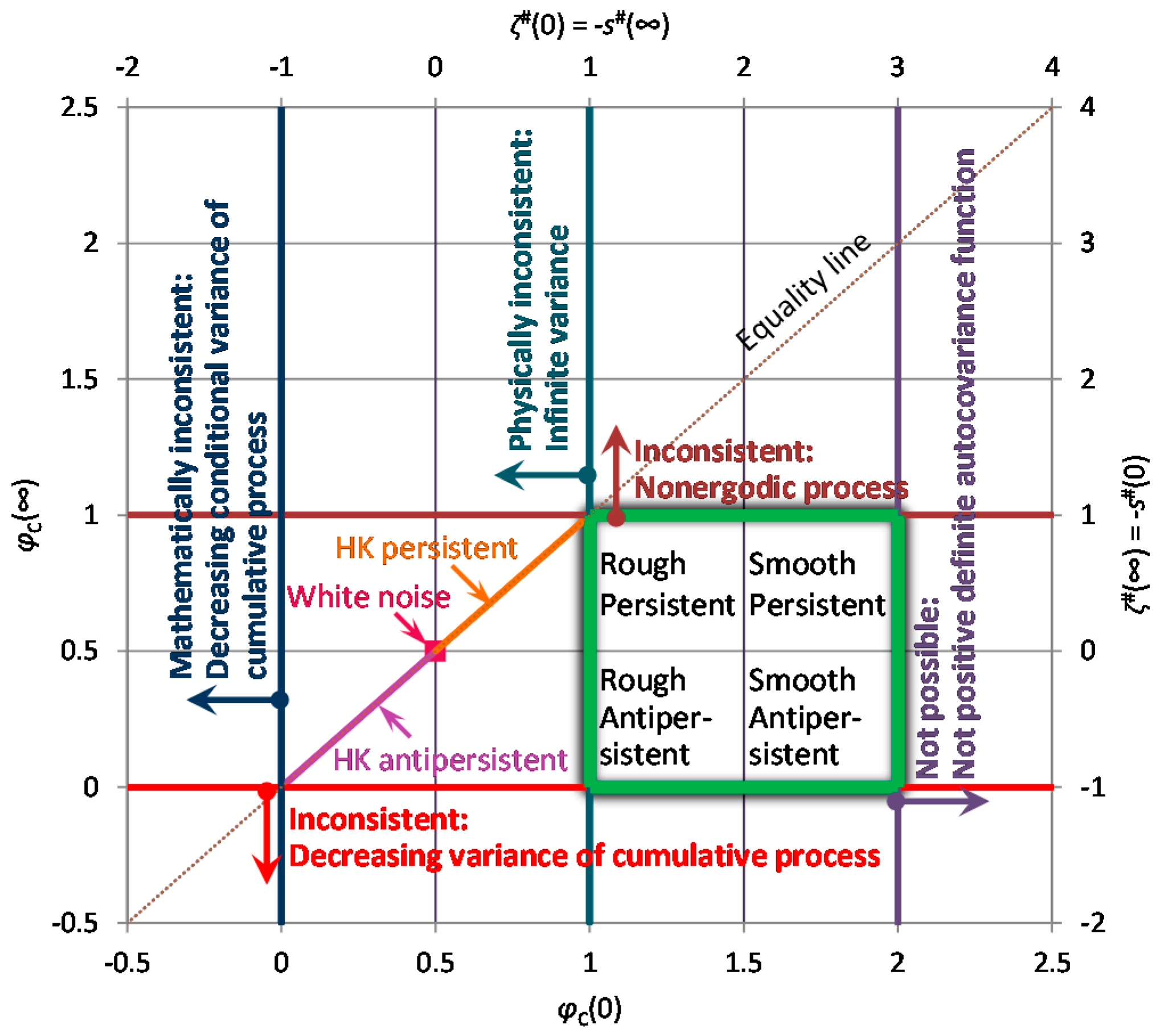
Because of the relationship of the entropy production with the scaling exponents, the bounds on the spectrum slopes translate directly into bounds of the CEPLT, i.e., and . These define the “green square” of admissible values of φC in Figure 2, which is also depicted in terms of admissible values of slopes ζ# and s# (noting that, as discussed above, s# can, by exception, take on values out of the square when or . The reasons why a process out of the square would be impossible or inconsistent, as discussed above, are also marked in Figure 2.
Large values of indicate a smooth process and small ones a rough process. Also, large values of indicate a persistent process and small ones an antipersistent process. The centre of the square, with coordinates represents a neutral process. As will be seen in next section, neutrality corresponds to a Markov process, which is neither rough nor smooth, and neither antipersistent nor persistent. Even though sometimes it is said to reflect short-term persistence, we must have in mind that a discretized Markov process at time scale k tends to be uncorrelated in time as k increases and therefore we may not have it in mind as persistent. In other words, here persistence is used as synonymous to long-term persistence, while high autocorrelations at small lags or scales, which die off at large lags or scales, are better described with the term smoothness. Both smoothness and persistence reflect high entropy production, locally and globally, respectively.
A useful observation in Figure 2 is that the entire “green square” lies below the equality line, which means that the same scaling exponent is not possible for both local and global behaviour, or else, it is impossible to have a physically realistic simple scaling process. There is one exception, the upper-left corner of the “green square”, which corresponds to the so-called “pink noise” or “1/f noise” and will be discussed further in Section 3.3.
Since we have pointed out several inconsistent or contradictory results that are reported in the literature, it may be useful to mention another case, which is frequently met in geostatistics. The so-called intrinsic models are common in geostatistics but susceptible to inconsistent use, even though the literature presents them as nonstationary to avoid some of the emerging problems. Such models are defined in terms of their structure function (variogram), v(h), which tends to infinity as lag h tends to infinity (e.g., [34]). An example is vI(h) = a hb with b > 0, in which we note that its formulation with respect to a single scalar argument, h, does not reveal the nonstationarity. Thus, it may be treated as if it was stationary. In that case, from (24) we have and thus the intrinsic process violates the constraint for physical consistency. Moreover, since vI(h) = γ0 − c(h) < ∞ for h < ∞, it turns out that c(h) = ∞ for any h and, hence, (21) entails that γ(k) = ∞ for any k. In other words, the infinity of is transferred to the entire autocorrelation function and the entire climacogram. In particular, the property γ(k) = ∞ means that the process is non-ergodic (in ergodic processes γ(k) should tend to zero as k tends to infinity; see [27] (p. 429)). Thus, in addition to being physically inconsistent such a treatment of the process is mathematically inconsistent and logically self-contradictory. A consistent way of treatment is to identify the intrinsic process with the (nonstationary) cumulative process X(t) [35], derive the stationary process x(t) and treat the latter further regularly. In that case the variogram is no longer related to the structure function of x(t) but to its climacogram; namely, it is identical to the cumulative climacogram vI(h) = Γ(h) = γ(h) h2.
Another peculiarity in geostatisical analyses is the so-called “nugget effect”, which is also problematic or enigmatic [36]. Namely, this is a discontinuity of the structure function at the origin. An example is vE(h) = a (h +c)b, h > 0, with c, b > 0, while vE(0) = 0. Investigation shows that the “nugget effect” does not necessarily create inconsistency. It is obviously associated with an infinite derivative of the structure function at the origin, i.e., . However, the LLD, can be finite at the limit as h → 0 (because of the multiplication by h). Therefore, the resulting does not necessarily lie out of the “green square”.
Figure 3 illustrates both the “intrinsic” case and the “nugget effect” and provides hints how to avoid both, adopting much better modelling alternatives. The above example of vE(h) was used with parameters indicated in the figure caption. It is easy to find that a FHK-C model which is both persistent (H = 0.75 > ½) and rough (M = 0.2 < ½) can replace the vE(h) and be used further.
Conversely, we can imagine that in the model identification and fitting of vE(h), persistence was regarded as an “intrinsic” characteristic and roughness was interpreted as “nugget effect”. Note that because M < ½, . Thus, a rough process seems like if it exhibited the “nuggest effect”. However, if instead of the standard plot of the variogram, a logarithmic plot was made (also shown in Figure 3 with respect to the upper horizontal axis), then the “nugget” would disappear.
3. Results
3.1. Revisiting Earlier Results
In an earlier study (already mentioned, [22]) on subjects related to the present one, it was suggested that extremization of EPLT in a continuous time representation could determine the entire dependence structure of the process of interest based on simple constraints. The specific premises for EPLT extremization were:
- (a)
- Lebesgue background measure;
- (b)
- constrained mean μ and variance γ(1) at a specified (observation) time scale;
- (c)
- constrained lag-one autocorrelation ρ at the specified time scale;
- (d)
- an inequality constraint φC(t) ≥ φ(t) to ensure physical realism as, naturally, by observing the present and past state of a process, the future entropy is reduced, whereas as t → ∞ conditional and unconditional entropies should tend to be equal, which, however, cannot happen if the entropy production is consistently lower in the conditional than in the unconditional case;
- (e)
- extremization of entropy production at asymptotic time scales, i.e., t → 0 and t → ∞.
These premises after systematic analyses resulted in two processes extremizing entropy production:
- A Markov process:maximizes entropy production for small times (t → 0) but minimizes it for large times (t → ∞).
- A Hurst-Kolmogorov (HK) process:maximizes entropy production for large times (t → ∞) but minimizes it for small times (t → 0).
In these definitions α and λ are scale parameters with dimensions of [t] and [x2], respectively. The parameter H, known as the Hurst parameter, determines the global properties of the process with the notable property:
Here we revisit these results as well as the premises, in light of the theoretical analyses of the previous section and incorporating empirical experience based on various data sets. These allow the following notes:
- The minimal entropy production of the HK process at small times may not be plausible for complex processes; rather we should generally expect that complex processes maximize entropy production at both small and large times (asymptotically as t → 0 and ∞).
- The HK process is characterized by infinite variance (, which, as discussed in the previous section, makes it physically inconsistent.
- The premise φC(t) ≥ φ(t) should certainly hold asymptotically (for t → 0 and t → ∞) but not necessarily at intermediate times. A specific example is the process shown in Figure 4h which includes a periodic component where the curve of φC(t) intersects that of φ(t) (the latter is not shown in the figure), even though asymptotically the inequality holds. It can thus be conjectured that if a process incorporates a deterministic component (e.g., periodic) while it is treated stochastically without separating the deterministic component, the inequality for EPLT and CEPLT could be violated at intermediate times.
- While the Markov process represents the maximal EPLT as t → 0 (φ(0) = 1), this property is shared by many other processes (see next subsection). Furthermore, in terms of CEPLT, while the Markov process corresponds to φC(0) = 3/2, there are processes which have higher CEPLT than the Markov, up to φC(0) = 2. These are smoother than the Markov process and have structure function with v#(0) = ξ#(0) > 1, where the value 1 corresponds to the Markov process.
Based on these remarks, the Markov process remains a valid candidate of physically consistent processes maximizing entropy production, if only the local asymptotic behaviour is of interest. However, additional constraints to the above premises (a)–(e) (from [22]) are needed to confirm its appropriateness, both on small scales (to enable determination of φC(0)) and large scales (to enable determination of φC(∞) = φ(∞)).
On the contrary, the HK process should not be regarded as a candidate of general validity, even though it is valid for large scales. Indeed, it is still quite useful as it results in high entropy production at large scales, a property that cannot hold for processes with exponential decrease of autocovariance such as the Markov process. We can thus regard the HK process as a useful mathematical construct which does not appear in nature but can be filtered appropriately to make a physically consistent process. This is the same with white noise (WN), which again is not physically consistent as it involves infinite variance in continuous time (see the specific location and the relationship of the WN and HK processes in the diagram of Figure 2).
It is well known that if a WN process is the input to a moving average filter , then it produces a physically consistent process with finite variance and autocovariance linearly varying in the interval [0, 2T] ([27] (p. 325)). Also, if is the input to a linear system corresponding to the linear differential equation , then the output is a Markov process ([27] (p. 326)), physically consistent.
Likewise if in these two cases the input is an HK process, then it is easy to see that the filtered output is a physically realistic process with finite variance γ(0), practically unaffected climacogram γ(k) at large scales, with γ#(∞) = 2H − 2 (as in the original HK process) but highly modified climacogram at small scales, thus having a valid structure (and climacostructure) function with v#(0) = ξ#(0) = 2H.
3.2. Specific Processes
Following the theoretical analyses of Section 2 and the remarks of the Section 3.1, we describe here a number of stochastic processes specified through any of their second order functions. All of these processes respect the limitations discussed in Section 2.4 and thus they are consistent mathematically and physically. Some of them correspond to high entropy production, but we also discuss processes with low entropy production. The complete details of these processes, along with graphs illustrating their properties and results of their application, are contained in Appendix A.2.
We start with a general Filtered Hurst-Kolmogorov (FHK) process (which in some cases, e.g., [24], has also been called the Hybrid Hurst-Kolmogorov—HHK—process). In Section 3.1 we briefly discussed two types of linear filters to the HK process, whose asymptotic properties are determined based on a single parameter, H. Here we generalize this result also making the asymptotic behaviour on the left independent from that on the right (cf. [37]) through introducing another parameter denoted as M (in honour of Mandelbrot, following [31]) which is called the smoothness (or fractal) parameter. We avoid specifying the linear filter needed to convert the HK process into the types of the FHK process given as this is not necessary (and in some cases it would be too involved). Rather we specify these types in terms of a convenient expression of the climacogram. The first case is defined through a generalized Cauchy-type climacogram (FHK-C) (see also [24]):
Both M and H are dimensionless parameters, and M and 1 − H vary in the interval (0, 1] with M < ½ or > ½ indicating a rough or a smooth process, respectively, and with H < ½ or > ½ indicating an antipersistent or a persistent process, respectively.
The second case is defined through a Dagum-type (FHK-D) climacogram:
and, despite its different expression, its behaviour, as well as the meaning and ranges of parameters are the same as in the Cauchy-type climacogram. For M = 1 − H both result in precisely the same special case:
The third case is obtained by summing a Cauchy-type climacogram with M = 1 and a Dagum-type climacogram with H = 0. The climacogram of the thus produced model (FHK-CD) is:
This is a convenient form, in which the first additive term determines merely the persistence of the process and the second one the smoothness of the process. In addition, it is more flexible and richer than its constituents, as it contains two couples of scale parameters; however, if parsimony is sought, then it can take the same number of parameters as each of the constituents by setting α1 = α2 and λ1 = λ2 (note that, for dimensional consistency, one λ and one α are minimal parameter requirements).
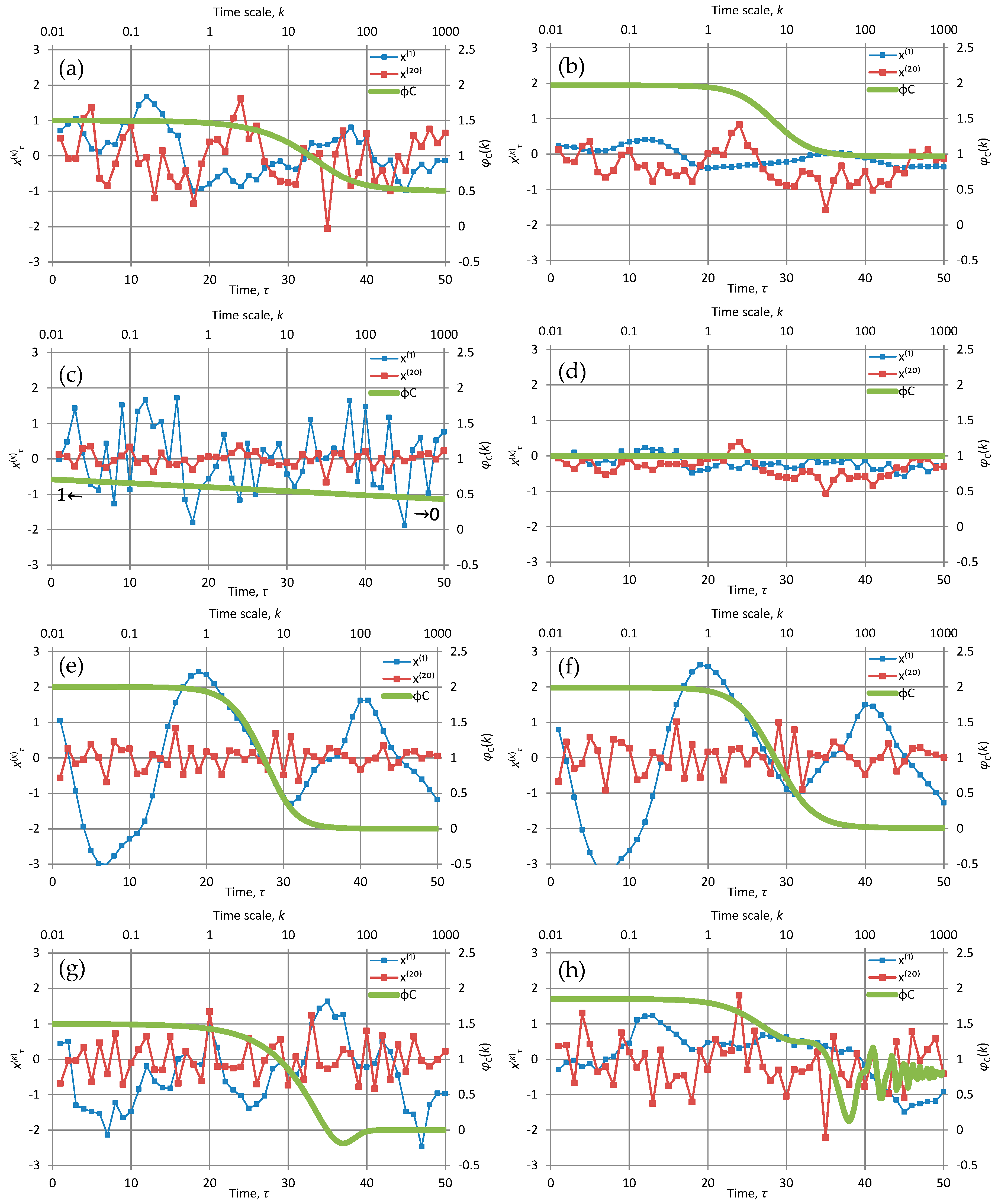
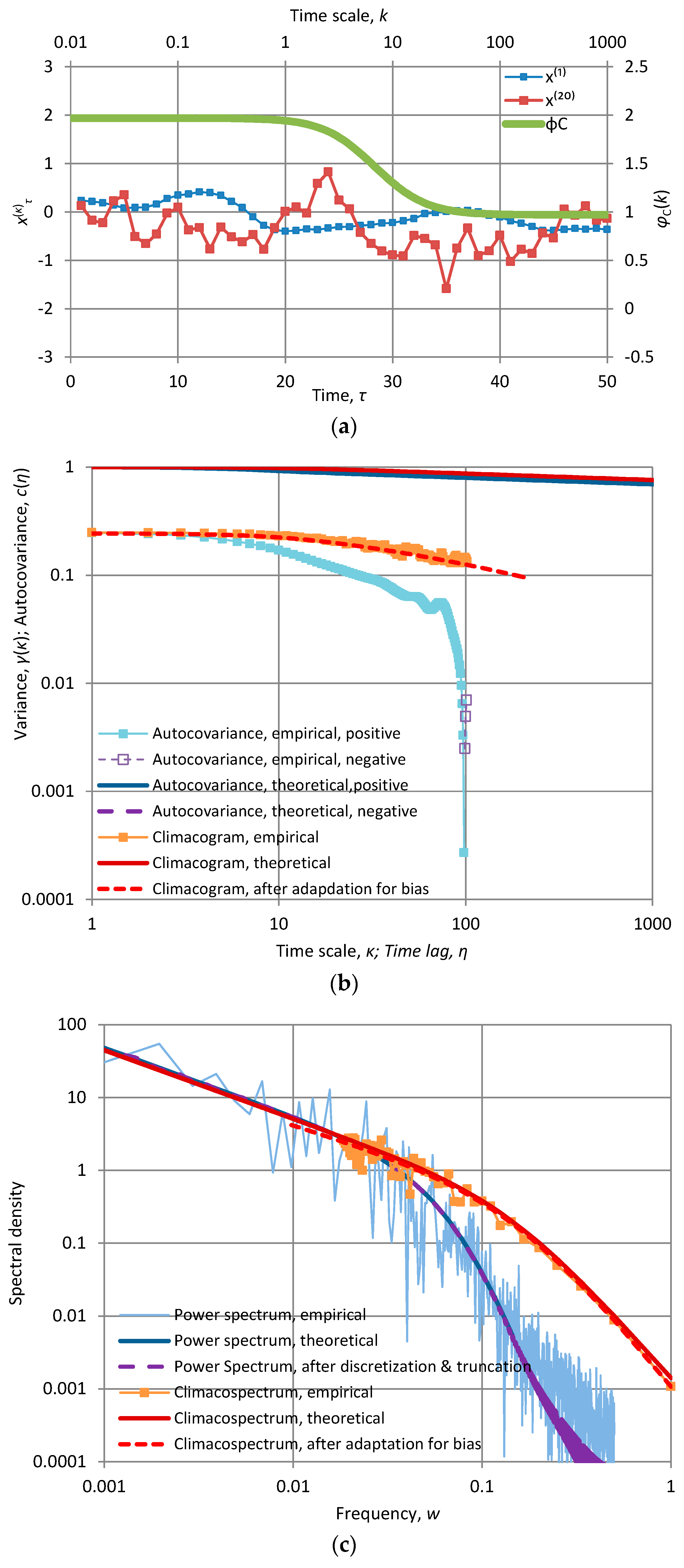
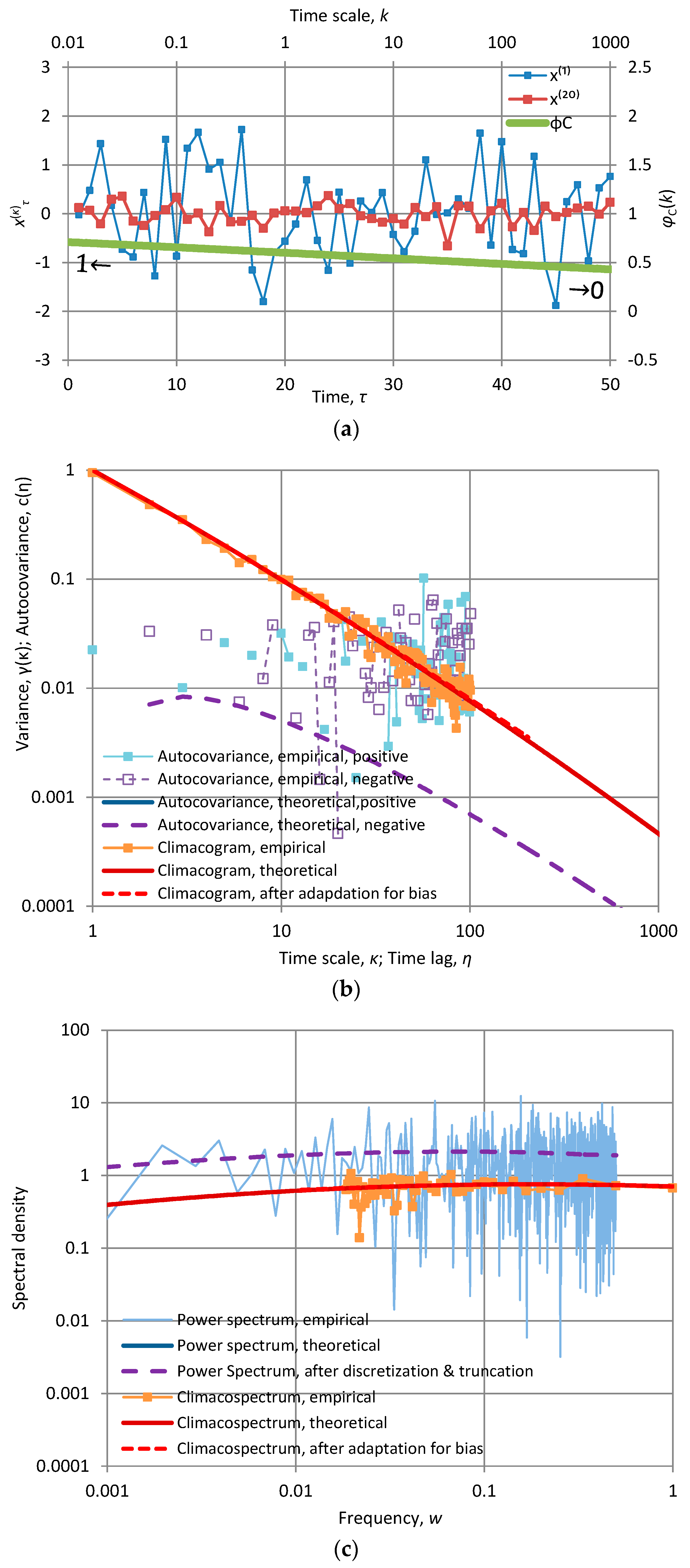
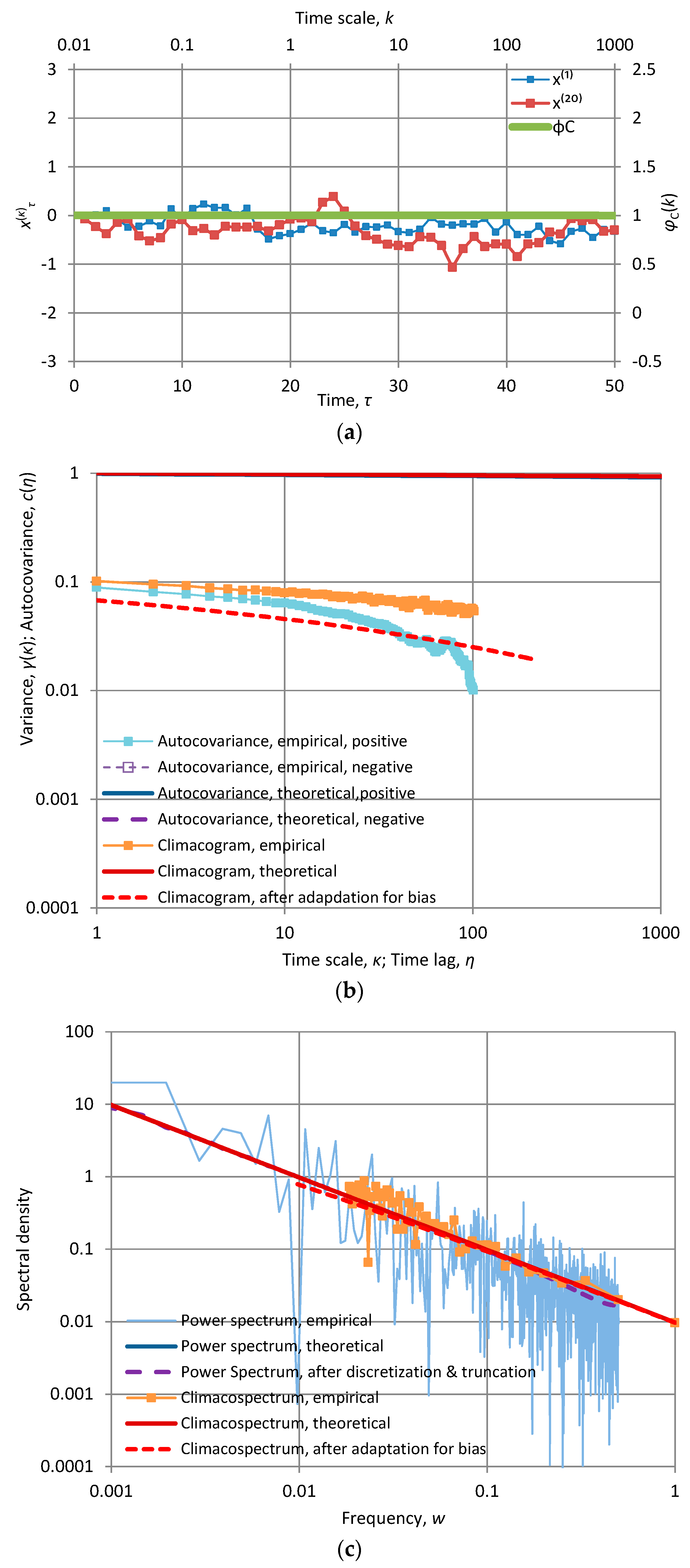
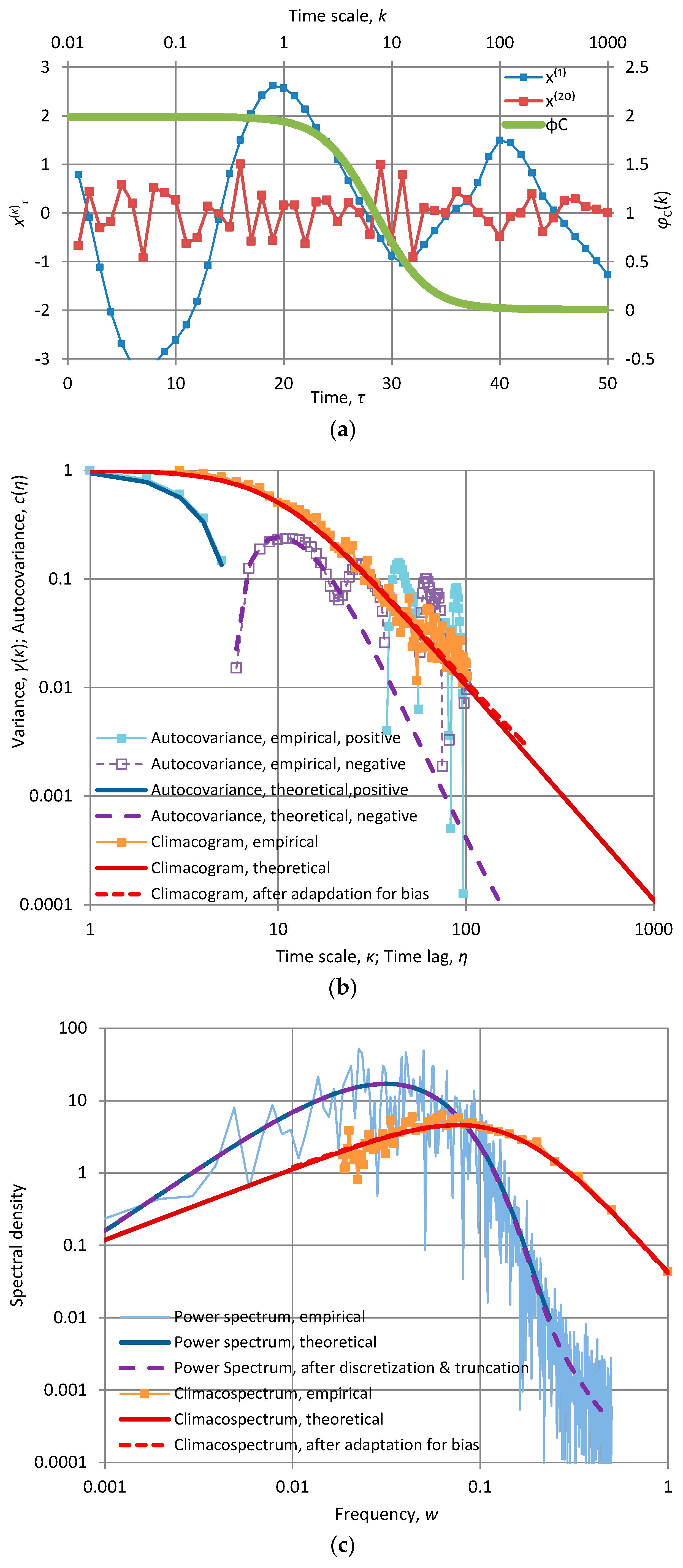
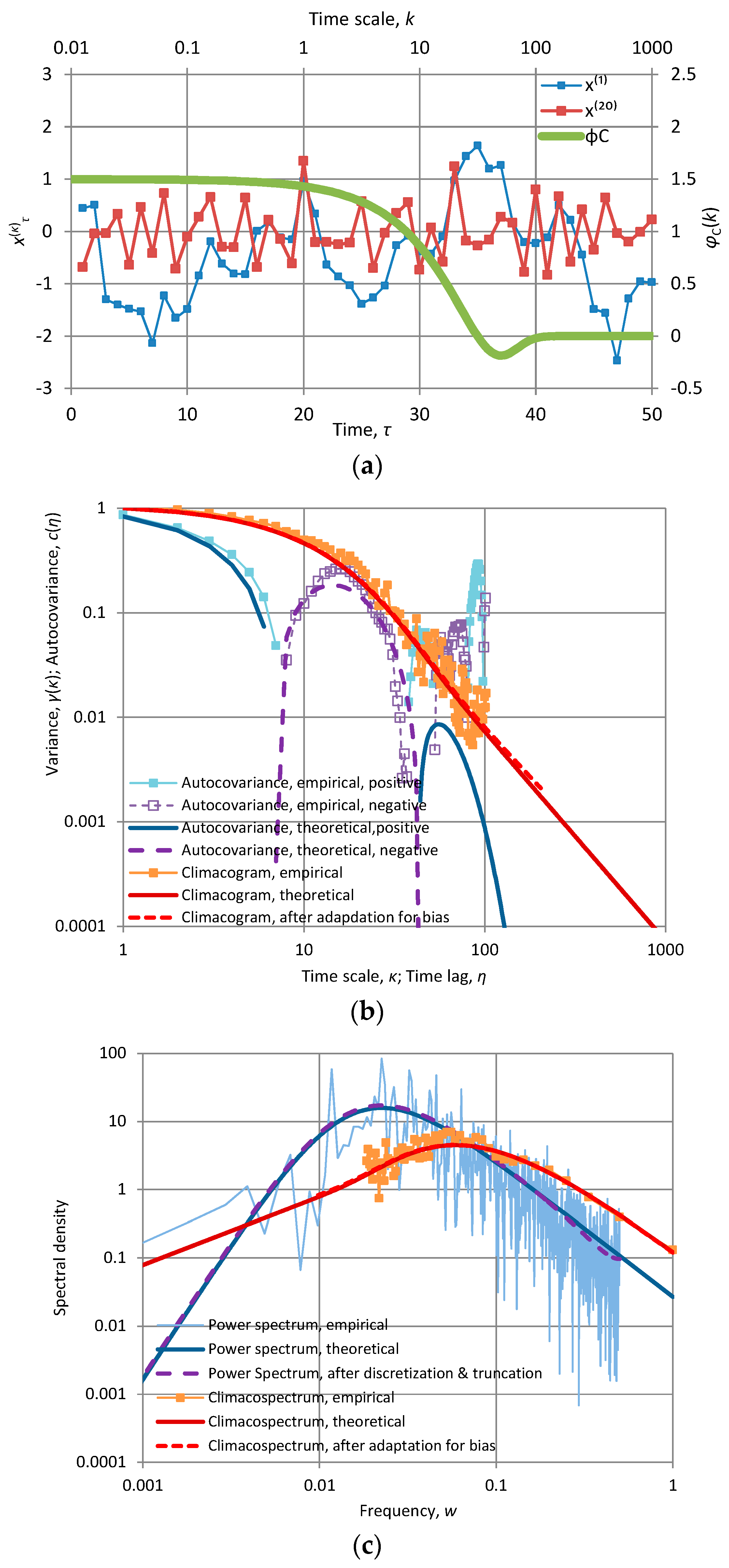
Even in its most parsimonious form, the FHK in any of the above three variants can cover the entire admissible range, i.e., the entire “green square” in Figure 2. The different patterns in time series generated by different M and H (specifically for the Cauchy-type climacogram) are illustrated in some plots of Figure 4 also in comparison with other models, first of which is the most customary Markov model (Figure 4a). The Markov model is good as a benchmark for comparisons because, as already discussed in Section 2, it is fully neutral (neither rough nor smooth as φC(0) = 3/2, and neither antipersistent nor persistent as φC(∞) = 1/2).
Each of the panels shows the first fifty terms of time series produced by each of the model implementations at time scales k = 1 and 20. In addition, each panel contains a “stamp” of the specific model represented by the plot of CEPLT, φC(k). Additional plots for all second order tools of each of the models are given in Appendix A.2. The time series for these models were generated quite easily using the generic model proposed in [24]; their length is 1024 and this is also the length of the series of coefficients a used for the generating symmetric moving average (SMA) scheme. All calculations are of algebraic type (based on the equations of Section 2 and Appendix A.2) and were performed in Excel spreadsheets without difficulties.
In Figure 4b the CEPLT is close to the absolute maximum both for small and large scales (H = M = 0.97 so as to obtain φC(0) = 1.97 ≈ 2 and φC(∞) = 0.97 ≈ 1); notable is the very smooth shape at scale 1 and the large departures from the mean (which is 0) at scale 20. On the contrary, in Figure 4c the CEPLT is close to the absolute minimum for all scales (H = M = 0.05, so as to obtain φC(0) = 1.05 ≈ 1 and φC(∞) = 0.05 ≈ 0—for better visualization it was preferred not to use values of H and M < 0.05). Furthermore, in Figure 4d the CEPLT is close to the absolute maximum for large scales (H = φC(∞) = 0.99 ≈ 1) and close to the absolute minimum for small scales (M = 0.01 resulting in φC(0) = 1.01 ≈ 1). Finally, in Figure 4f the conditions are opposite to those in 4d, i.e., the CEPLT is equal to the absolute minimum for large scales (H = φC(∞) = 0.01 ≈ 0) and to the absolute maximum (2) for small scales (M = 0.99 resulting in φC(0) = 1.99 ≈ 2).
The particular case of Figure 4d is close to what is usually called “pink noise” or ”1⁄f noise”, as the power spectrum has almost constant slope −1 for the entire frequency domain (which is the same in the climacospectrum). This means that using the FHK model we can theoretically represent and practically produce even “pink noise” in a consistent stationary setting without linking it to a nonstationary process [38,39], which actually involves several theoretical inconsistencies [31]. Indeed, as can be seen more thoroughly in the detailed graphs of Figure A5 in Appendix A.2.2, which are for the same application with that of Figure 4d, the small change of slope of from 0.99 to 1.01 is not actually visible, especially in view of the very rough shape of the empirical periodogram, which certainly cannot support differentiation between 0.99 and 1. The FHK model can be used also in other ways to produce “pink noise”, that is, by selecting a very large (small) parameter α so as to expel from our field of vision the asymptotic behaviour on large (small) scales. And we can imagine that in several cases of empirical explorations using observations of natural processes, the observation resolution and length, compared to characteristic scale(s) of the process, are such as to hide the asymptotic behaviour of the process.
We can use this as a trick to obtain virtually constant power spectrum slopes much steeper than −1. This is illustrated Figure A7 of Appendix A.2.2 where the FHK was used with H = M = 0.75 and α = 100. These yield theoretical slopes and . However, the large α does not allow viewing the asymptotic behaviour at low frequencies or large scales and the slope dominates everywhere. Actually the empirical periodogram estimates an even steeper constant slope, s# = −2.6. This should not mislead us to conclude that the process is nonstationary because the slope is steeper than −1 (as happens in many studies in the literature). Likewise, in the case that the time series represented observations of a natural process, such a result must not be misinterpreted as evidence that natural processes can lead to slopes constant for all scales and steeper than −1. Clearly here, the process is stationary, the slope −2.5 refers to large frequencies or small scales but, because of the large characteristic scale and the limited observation period (1024 in this example), we cannot see what happens at larger scales. If we saw, then the slope would be −0.75, in accord with the theory.
As discussed, the Markov process is neutral but, by modifying its power spectrum, we can obtain processes which are smooth or antipersistent. Two types of modifications are studied in Appendix A.2, introduced in terms of their power spectrum, i.e.,
and:
where n = 0, 1, 2…, and the value n = 0 results precisely in a Markov process. For n > 0, (60) corresponds to a smooth process with φC(0) = 2 and (61) corresponds to an antipersistent process with φC(∞) = 0. The resulting autocovariance function retains the characteristic exponential form of the Markov process but is multiplied by a polynomial function of lag (see Appendix A.2). Therefore, we call these two processes the smooth exponential (SE) and the antipersistent exponential (AE), respectively. In each of the cases, a most extreme value of CEPLT is achieved (maximal for small scales in SE and minimal for large scales in AE). Figure 4g, shows an example of AE for n = 2; the hole in the function φC(k) for moderate k is a characteristic of this process.
An interesting process that is simultaneously extremely smooth (φC(0) = 2) and extremely antipersistent (φC(∞) = 0) is defined by the following power spectrum:
where cn is a normalizing constant making the area of the power spectrum equal to . This process, which we call generalized Planck (GP) is obtained by a generalization of Planck’s law of black-body radiation, whereas it is identical to this law if n = 1. The detailed equations of this process are also given in Appendix A.2. A characteristic plot of time series generated from this process is shown in Figure 4e, and is almost indistinguishable from Figure 4f which, as already discussed, was produced as an approximation by FHK.
A final case examined in the Appendix A.2 is a harmonic oscillation, which is very easily modelled as a deterministic process but here it is treated as a stochastic process. Of course stochastic treatment is not advisable in this case, but often such periodic behaviours appear as components of stochastic processes. Obviously the second-order characteristics of such processes are affected by periodic components and therefore we need to know which equations should be superimposed in those of the pure stochastic process (see also [40,41]). As an example of such a case, Figure 4h shows the behaviour of a process defined as the average of a FHK with H = M = 0.8 and a harmonic oscillation. It is difficult to identify the presence of the oscillation from visual inspection of the time series, but the detailed graph of any of the second order characteristics, plotted in Appendix A.2., captures the periodic behaviour.
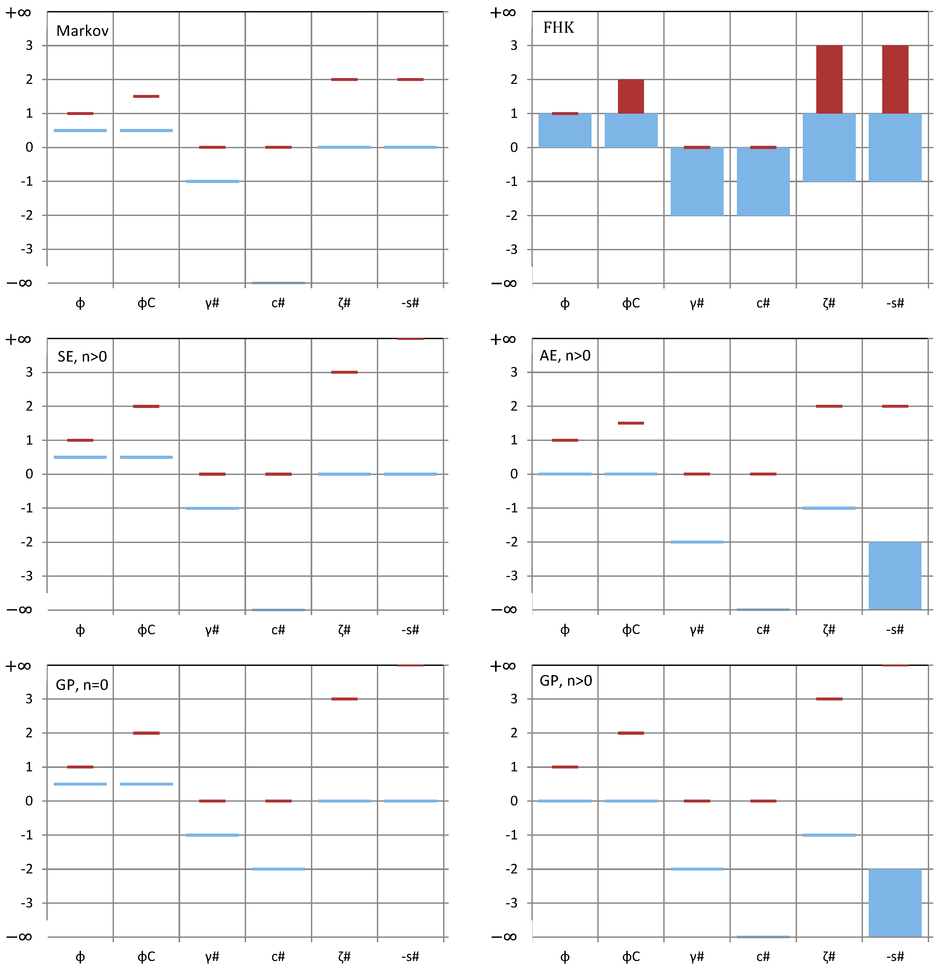
3.3. Comparison of Asymptotic Properties
Most of the models examined in the previous subsection can only reproduce specific values of asymptotic properties. An exception is the FHK model which is the most powerful as it can perform in the entire admissible domain of asymptotic properties. A visual comparison of all models examined, it terms of the asymptotic values of the different second order characteristics is made in Figure 5, while Figure 6 provides an envelope for all models, with classification of the ranges in terms of smoothness and persistence.
Further comparative information about which model can perform for the most extremal cases is provided in Table 4. These figures and the table can be useful for the model selection based on data.
3.4. Real World Case Study
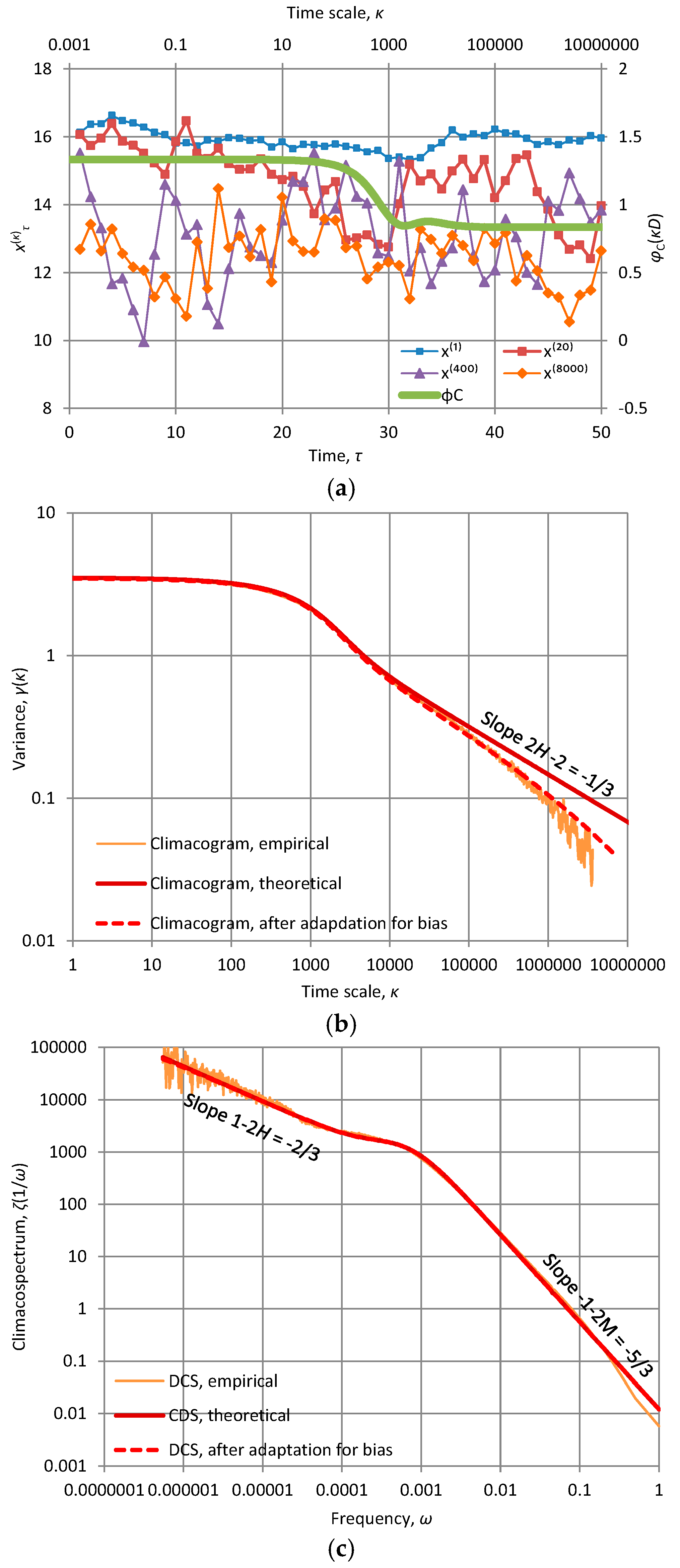
Empirical testing of the theoretical analyses presented here needs fine resolution of measurements and long time series, in order to reliably determine the asymptotic properties from data. Geophysical time series usually do not satisfy either of these two conditions. However, laboratory measurements of turbulent velocity can meet the conditions. Indeed, in laboratory experiments at sampling intervals of μs, very large samples can be formed which can enable viewing the asymptotic behaviour. Here we use grid data of nearly isotropic turbulence from the Corrsin Wind Tunnel at a high-Reynolds-number [42], which were made available on the Internet by the Johns Hopkins University. This dataset consists of 40 time series with n = 36 × 106 data points of wind velocity along the flow direction and an equal number of time series of cross-stream velocity, all measured at a sampling time interval D = 25 μs by X-wire probes placed downstream of the grid. Here we use part of the data, namely the series of wind velocity along the flow direction at the first of the probes (first column of files in http://pages.jh.edu/~cmeneve1/datasets/Activegrid/M20/H1/). More data and analyses have been used by Dimitriadis and Koutsoyiannis [43] at a somewhat different context.
Characteristic plots of the turbulent velocity time series are shown in the Figure 7a for various time scales. The large persistence of turbulence is evident from the large variability at the largest time scales. Impressively, an FHK-CD model with five parameters describes well the data at the entire range of available time scales which spans almost seven orders of magnitude.
The fitted model parameters are: H = 5/6 = 0.83, M = 1/3 = 0.33, a1= a2 = 2170 D = 54 ms, λ1 = 1.13 m2/s2, λ2 = 2.39 m2/s2. These confirm the intense persistence and a small roughness, which is reflected in a climacospectrum slope of −5/3 for large frequencies (the neutral would be −2), in accord with Kolmogorov’s theory.
4. Discussion and Conclusions
The question whether the probabilistic (information) entropy incorporates, as a special case, thermodynamic entropy or the two are different concepts, is still debated [44,45]. If we adopt the former proposition of the dilemma, as we have done here, the requirement emerges that entropy production should be formulated in a stochastic context, while current attempts mostly use the classical thermodynamic entropy definition as in heat transfer. This is not an easy task and certainly requires exploration of a broad spectrum of alternatives for a definition of the concept of entropy production. Exploration of extremum principles for entropy production in a stochastic framework is also crucial. The two versions proposed here, entropy production in logarithmic time, unconditionally (EPLT) or conditionally on the past and present having been observed (CEPLT), may have some usefulness and potential as explanatory and modelling tools. The findings of this study include the following:
- Definition of entropy production with respect to logarithmic time has some attractive characteristics and is consistent with the notion of the time arrow.
- The asymptotic values of entropy production for time zero and infinity seem to be crucial for its extremization and define important features of a process.
- In particular, the asymptotic value of CEPLT for zero time defines the roughness (fractality) of the stochastic process while the common asymptotic value of EPLT and CEPLT for infinite time defines the (long-term) persistence of the process and equals the Hurst parameter.
- Both ELPT and CEPLT are finite and constrained within specific theoretically justified bounds. The scaling laws of all second order characteristics of stochastic processes are a result of these finite values and are also subject to bounds (with few exceptions fully described). The proofs of existence of these bounds offer the means to fight common misunderstanding, misuse, false reporting and inconsistent estimation of characteristics of geophysical processes, as well as to develop consistent estimation algorithms.
- The climacogram and its derivative tools introduced here, namely, the differenced climacogram and the climacospectrum are very powerful and support the estimation of entropy production, in either of its forms, from data series.
- The broad family of models for stochastic processes investigated here covers the entire admissible range of asymptotic behaviours and offers the means for modelling any type of processes, either using a single model or a combination of more than one model.
- The real-world application presented with the extraordinary long time series of turbulent velocity shows how a parsimonious stochastic model can be identified and fitted using the tools developed.
Measurements of diverse turbulent phenomena can potentially provide equally long time series with fine resolution, shaping a broader empirical basis for future work on identifying natural behaviours, specifically on larger spatial and temporal scales, and further testing the adequacy of the models. Characteristics of order higher than second, along with the effects of non-Gaussianity on entropy production, are also interesting to examine in light of the developments for second-order ones. A recent study [43] has already provided interesting results with respect to high-order moments. Connections of microscale turbulence and macroscale atmospheric phenomena are also a broad field for future studies. Further applications, also extending similar recent works in hydrology, geophysics and ecosystems [30,40,41], would enrich our knowledge on natural behaviours.
Acknowledgments
I thank Huijuan Cui, Bellie Sivakumar and Vijay P. Singh for the invitation to write an article for the Special Issue, and the two anonymous reviewers for the encouraging and constructive comments. I gratefully acknowledge discussions about several issues on stochastics covered here with members of the Itia research team, colleagues and friends, and particularly with Panayiotis Dimitriadis, Federico Lombardo, Spencer Stevens, Any Iliopoulou, Hristos Tyralis, Andreas Efstratiadis, Katerina Tzouka, Georgia Papacharalambous, Panagiotis Kossieris, Yannis Tsoukalas, Andreas Langousis, Yannis Markonis, Christoforos Pappas, Simon Papalexiou, John Halley, Elena Volpi, Yannis Dialynas, Ilias Deligiannis, Harry Lins, Christian Onof, Alin Carsteanu, Amilcare Porporato and Alberto Montanari, and earlier with Tim Cohn and Vit Klemes who are no longer with us.
Conflicts of Interest
The author declares no conflict of interest.
Appendix A
Appendix A.1. Derivations and Theoretical Details
Appendix A.1.1. Properties of the LLD
Here we examine some asymptotic properties of the log-log derivative of general validity, which are useful in other derivations herein. First we examine the product of two functions, i.e.,
By applying the definition of LLD (Equation (38)) and using standard calculus, it is easy to show that:
which we can conveniently denote as:
Likewise, it is easily shown that:
By setting in (A3) (constant), and observing that , it is easily verified that:
By setting in (A3) it is easily verified that:
and likewise, extending for any exponent λ:
We now examine the sum of two functions, i.e.,
By applying the definition of LLD and using standard calculus, it is easy to show that:
In other words:
Finally, we examine the composition of two functions, i.e.,
Again by applying the definition of LLD and using standard calculus, we easily find:
Appendix A.1.2. Proof of the Positive Definiteness of the Climacogram
We will demonstrate that γ(k) is a positive definite function based on the well-known fact that the autocovariance function c(h) is positive definite. It suffices to show that the Fourier transform of γ(k), i.e.,
is positive. Expressing γ(k) in terms of c(k) from (21) we have:
Setting χk = ψ, χdk = dψ, we find:
and invoking the definition of the power spectrum as the Fourier transform of c(h) (Equation (10)), we get:
Both quantities s(w/χ) and (1 − χ)/χ are positive for 0 < χ < 1 and thus .
Appendix A.1.3. Proof that the Differenced Climacogram Is Nonnegative
First we will prove a more general inequality that will be used for the proof, i.e.,
With reference to the cumulative process, as seen in Figure 1, we have:
and since , we find:
or, taking the square roots as the quantities are positive:
By substituting Γ(h) = h2 γ(h) we get (A17). As a corollary, by setting r = h we derive:
which ensures that the differenced climacogram is nonnegative.
Appendix A.1.4. Determination of the Characteristic Constant ε of CEPLT
From (41) and the condition put as desideratum (i.e., that, as k → ∞, , it follows that:
Now assuming that b = , it follows that the limit:
is finite. Likewise:
By dividing the last two equations we find:
and finally:
which proves (42).
Appendix A.1.5. Asymptotic Properties of CEPLT
The fact that follows directly from the definition. For the LLDs, starting from the definition of the differenced climacogram we proceed as follows:
Hence, by virtue of (A3):
According to the derivations in Appendix A.1.4, the quantity in parentheses has a finite limit as k → ∞, which specifically is . Thus, its LLD tends to zero as k → ∞ (see explanation in the last paragraph in Appendix A.1.8) and hence . Likewise, because (finite). However the term in parenthesis is nonzero for k → 0, so to determine the asymptotic behaviour of in that case we follow a different path.
Specifically, we can express in an alternative manner in terms of the climacostructure function. Using the definition of the latter, we can write:
Hence:
Proceeding as above we derive:
and hence the quantity in parentheses in (A30) has a finite limit as k → 0, which specifically is . Thus, its log-log derivative tends to zero as k → 0 and hence .
We further note that from the definition of the climacostructure function and using Equation (A10) we get:
As k → ∞, the numerator is zero, while the denominator is γ0, so that . The concluding remark is that, because , none of the two tools, climacogram and climacostructure function suffices alone to express both the local and global asymptotic properties of . On the other hand, the combination of the two suffices.
Appendix A.1.6. Area of Climacospectrum
From the definition of climacospectrum (48), the entire area under it is:
By changing variable, setting k = 1/w, dk = −(1/w2) dw, we get:
We will evaluate A by taking the limit as x → 0 of:
The latter can be written as:
so that:
For small x, because γ(k) is finite for any k and we are interested about the limit of A(k) as x → 0, at the limit we can replace γ(k) with γ(0) and get:
For completeness we note that, as can be easily seen, the integral:
evaluates to:
However, this is finite only for antipersistent processes, while it diverges to +∞ for persistent processes.
Appendix A.1.7. Details and Derivation of the Inverse Transformation of Climacospectrum
Combining both forms of (49) we find:
or by setting k = 2x:
and this is valid for any x. This means that the function ζ(x) cannot take any arbitrary form but its form should be such that (A42) is satisfied for any x. At the same time, as shown in Appendix A.1.6:
where for the very last term we used the transformation k = 2x, dk = (ln 2) 2x dx. Combining (A42) and (A43) we find that, for any k:
Note, however, that the equality of the sum with the integral holds only if both limits for summation and integration are infinite. It can be used also as an approximation for small k, by setting the lower integration limit to k; thus the following approximations hold:
where has been defined in Equation (50). Combining these two cases we heuristically derive the left part of Equation (50), which was shown by an extensive numerical investigation to be almost indistinguishable from the exact solution (49). The advantage of (50) over (49) is that, to calculate a sufficient approximation by (49), we need to go to very large time scales (2i k), which may not be feasible when working with data series, while (50) can perform well in reasonably smaller time scales. In numerical applications, the evaluation of the integral I(t) goes sequentially from large to small time scales. To start the calculation, for the largest time scale k = q we exploit the second case of (A45) and get I(q) = 2 ζ(q)/q. It should be kept in mind that both I(k) and ζ(k)/k are decreasing functions of k for large scale. Even if we assumed that ζ(k)/k is constant, rather than decreasing, for a range of scales close to q, we would derive from the second case of (A45) that I(q − iD) = (I(q)/q) (2 + 1/(q/D − 1) + … + 1/(q/D − i)), which clearly shows that I(q) is a decreasing function of k.
Appendix A.1.8. Remarks on Asymptotic Scaling
We maintain that every nonzero continuous function f(x) defined in (0, ∞), whose limits as x → 0 and x → ∞ exist, is associated with two asymptotic power laws, or else two asymptotic scaling behaviours, one on each of the two ends, 0 (local scaling behaviour) and ∞ (global scaling behaviour). To prove this, first we examine the asymptotic behaviour of f(x) as x → ∞ and we try to identify the first asymptotic law. We perform the following steps:
- We find . If then we replace f(x) with , otherwise we keep it as it is. Clearly then, .
- We find . If then we replace f(x) with ln|f(x)| (which preserves the property ); if necessary, we make iterations so that eventually and .
- Given the properties in point 2, there exists a unique b, 0 < b < ∞ satisfying:so that for any b′ ≠ b:
- The constant b defines an asymptotic power law with exponent b (cf. Hausdorff dimension; the case b = 0 signifies an improper scaling).
To identify the second asymptotic law as x → 0, we define and we proceed in the same manner to construct a function satisfying the conditions in point 2 above. Proceeding likewise, we determine the unique a for which . This an asymptotic power law with exponent a for f(x) as x → 0.
We remark that the two power laws refer to the same function f(x) but, due to the replacement steps of the procedure, may eventually correspond to different functions, say, fa(x) and fb(x) for the asymptotic behaviours as x → 0 (local behaviour) and x → ∞ (global behaviour), respectively. However, it is easy to construct a single function that combines both, making a final replacement, e.g., f(x) = fa(x)fb(x), but many different f(x) can actually be constructed. Thus, as well as any object has a dimension, any continuous function entails asymptotic power laws; generally not one but two, which in the special case of simple scaling can be identical.
Now, coming to the asymptotic values of for and ∞, symbolically f#(0) and f#(∞), these are:
To prove the former case, we proceed as follows:
This implies that and thus . The latter case () can be proved in the same manner.
A useful property is that if is a finite value (<∞), then , because for any b′ > 0, . Likewise, if is a finite value, then . Thus, to have asymptotic (for x → 0 and ∞) values of different for 0 and ∞, the asymptotic values of f should be either 0 or ∞. These properties are useful and are utilized in other proofs herein.
Appendix A.1.9. Asymptotic Scaling of the Different Second Order Tools
We assume that the asymptotic behaviour of the climacogram-based second order tools is given as:
and we will determine that of the autocovariance-based tools. Note that the equality of the different function limits in (A50) has been proved in Appendix A.1.5.
We will fist examine the asymptotic properties of the autocovariance function. Initially we note that, because γ(0) = c(0) = γ0 (finite), it follows that γ#(0) = c#(0) = 0. Now, since b = < 0, it follows that:
where c is finite. We use the relationship between γ(k) and c(h) (Equation (21)) to find:
Because both and as h → ∞, applying l’Hôpital’s rule we find:
Since b < 0, , , and will also as h → ∞. Thus:
Unless b = −1 or b = −2, the limit is 0, finite or ∞, if and only if is 0, finite or ∞, respectively. Therefore, if b ≠ −1, −2, then , otherwise , which does not guarantee (nor does it exclude) that .
Next we will examine the asymptotic properties of the structure function. Initially we note that, because ξ(∞) = v(∞) = γ0 (finite), it follows that ξ#(∞) = v#(∞) = 0. Now, since a = > 0, it follows that:
where d is finite. We use the relationship between ξ(k) and v(h) (Equation (26)) to find:
Because both and as h → 0, applying l’Hôpital’s rule we find:
If a > 1, then both and will also as h → 0. In this case, again applying l’Hôpital’s rule:
If a < 1, then and will both as h → 0. Thus, again applying l’Hôpital’s rule, we will conclude with (A58) again. Thus, in both cases:
Since a > 0 the rightmost expression cannot be zero unless d = 0. Therefore, the limit is 0, finite or ∞, if and only if is 0, finite or ∞, respectively. Therefore, .
If a = 1 precisely, then (it does not tend to 0 or ∞), while . Thus, from (A56) we get = 3d (finite), which again means that . Also, if a = 2 precisely, then and from (A56) we get = 6d (finite). In conclusion, in all cases it holds that and , which means that v(k) has the same asymptotic behaviour with ξ(k) in both ends. We can thus rewrite (A50) as:
Now coming to the asymptotic behaviour of the power spectrum, according to Gneiting and Schlather [37] (who also cite [46,47,48]), the power spectrum is “typically” associated with the asymptotic relationship s(w) ~ w−a−1 as w → ∞ and s(w) ~ w−b−1 as w → 0, where a (>0) and b (<0) are the LLDs of the structure function, v#(0) and autocorrelation function c#(∞), respectively, same to the above discourse. By inspection, it is seen that the slopes −(a + 1) and −(b + 1) are precisely the log-log slopes of the climacospectrum expressed in terms of frequency, , or equivalently and , respectively. It can be conjectured that, since this is the “typical” behaviour, the non-typical cases correspond to integral values of a and b.
In plain language, the above results can be expressed as follows:
- The asymptotic behaviour of the autocovariance function is the same with that of the climacogram.
- The asymptotic behaviour of the structure function is the same with that of the climacostructure function.
- The asymptotic behaviour of the power spectrum is the same with that of the climacospectrum.
Exceptions to the rule 1 may occur when b = −1 or b = −2 and this was indeed verified by thorough analytical work using the series of models examined in Appendix A.2. Exception to rule 2 can also appear and indeed they were found when b = −2 or a = 2. The entire list of exceptions found in this analytical work follows, also mentioning the specific models in which they appeared:
- and : Markov, Smooth Exponential models
- and : Generalized Planck model for n = 0
- and , also while −1: Antipersistent Exponential model for n > 0
- and , also while : Generalized Planck model for n > 0
- and while : Generalized Planck model
- = 2 and while : Smooth Exponential for n > 0
Appendix A.1.10. Proof of Physical Inconsistency of too Mild Slopes at High Frequencies in Power Spectrum
Let us assume that for small scales k < 𝜖 or high frequencies w > 1/𝜖, with 𝜖 however small, the log-log derivative is , or else s(w) ~ wβ where β is a constant satisfying . As the area of the power spectrum equals the variance of the continuous time process, we will have:
Because s(w) ~ wβ, there exist α > 0 so that s(w) ≥ α wβ for w > 1/𝜖. Thus the, rightmost of the above integrals can be evaluated as:
Clearly if as and thus γ(0) = ∞. The same result could be obtained if the climacospectrum was used instead of the power spectrum. Because infinite variance means infinite energy, which is physically inconsistent, it turns out that the assumption is physically absurd.
Appendix A.1.11. Proof of the Inconsistency of too Steep Slopes at High Frequencies in Power Spectrum
We prove that or, equivalently, , by contradiction, i.e., assuming with M > 1. In the latter case for small k we may approximate ξ(k) as:
which indeed yields . The climacogram for small k is thus:
The positive definiteness of γ(k) entails that any matrix A with elements ai,j = γ(ki − kj) should be positive definite. Choosing three points, ki = k0, k0 + k and k0 + 2k, we form the 3 × 3 matrix:
whose determinant can be easily evaluated. Specifically, after algebraic manipulations we obtain:
This can also be written as:
We observe that G(k, M) is a second-order polynomial in terms of y := k2M with discriminant , which is positive for any M > 0 and thus the equation G(k, M) = 0 has two real solutions:
Clearly, y1 < 0 for any M, while y2 < 0 only when M < 1 (for M = 1, y2 = 0 precisely). Therefore, if M > 1, then for 0 < k2M < y2, G(k, M) < 0 and hence B(k, M) < 0, which proves that A is not positive definite as its principal determinant is negative.
Solved for k, the interval where B(k, M) < 0 is:
This means that, if M > 1, B(k, M) is negative for arbitrarily small k (in the neighbourhood of 0), which justifies the approximation we have used for ξ(k). Therefore the assumption M > 1 should be rejected.
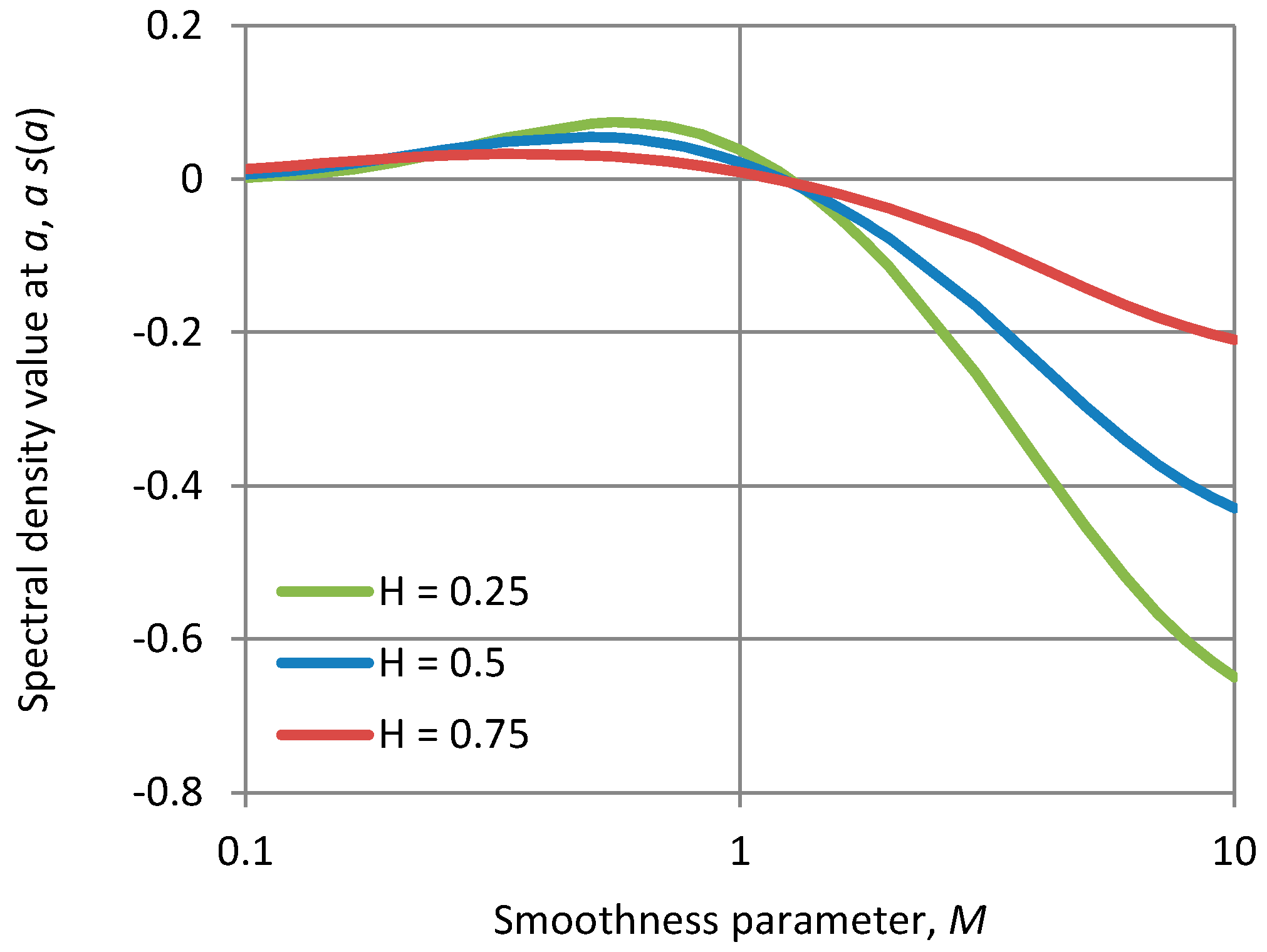
As an illustration by a different approach, Figure A1 shows for the FHK-C model, a single value of the power spectrum, namely s(α), where α is the time scale parameter of the model, as a function of the parameter . As seen in the plot, for M > 1, s(α) < 0 which confirms absence of positive definiteness, now of the autocorrelation function. (We note that for M > 1 but very close to 1, the plot shows s(α) slightly positive but in fact it is negative again for some w > α—not shown in the figure).
Figure A1.
Plot of the spectral density value at w = α, standardized by α, for the FHK-C model with smoothness parameter M varying in [0.1, 10] and for the indicated values of the Hurst parameter H.
Figure A1.
Plot of the spectral density value at w = α, standardized by α, for the FHK-C model with smoothness parameter M varying in [0.1, 10] and for the indicated values of the Hurst parameter H.

Appendix A.2. Specific Stochastic Models and Their Behaviour
In Appendix A.2 we provide detailed tables with mathematical expressions for all the models used in the paper and detailed graphs with applications of these models. All models include two scale parameters, α (scale parameter of time with dimensions of [t]) and λ (scale parameter of variance, with dimensions of [x2]). These are absolutely necessary for dimensional consistency. Some models contain additional dimensionless shape parameters, such as the smoothness parameter M, the persistence (Hurst) parameter H, or other as specified in each of the models. The theoretical characteristics depicted in the graphs are determined from the expressions given in the tables. The time series also depicted in the graphs, along with and their empirical characteristics, were produced by the SMA model as described in the text; their length is 1024 in all cases. For facilitating comparisons, in all applications the parameter α is the same, α = 10 (except if stated otherwise in the caption), while λ is chosen so that γ(1) = 1.
Appendix A.2.1. Markov Process
The Markov (also known as Ornstein–Uhlenbeck) process is the most convenient as all its second-order characteristics have simple expressions (see Table A1) and, simultaneously, the most parsimonious as it includes no other parameter additional to the two necessary scale parameters α and λ. For these reasons it is the most common in applications. On the other hand, its neutrality in terms of smoothness and persistence, and more specifically the low entropy production for large time scales, does not make it a good candidate to model natural behaviours.
The application depicted in Figure A2 corresponds to an unusually high lag-one autocorrelation (ρ = 0.94). Note that the model does not allow control of autocorrelation once the parameter α is specified.

Table A1.
Mathematical expressions of the second order characteristics of the Markov process and their asymptotic properties.
Table A1.
Mathematical expressions of the second order characteristics of the Markov process and their asymptotic properties.
| Characteristic | Mathematical Expression | Local Asymptotic Properties | Global Asymptotic Properties | Equation |
|---|---|---|---|---|
| Climacogram | (A70) | |||
| Climacospectrum | (A71) | |||
| Entropy production | (A72) | |||
| Autocovariance function | 0 | (A73) | ||
| Power spectrum | (A74) |
Figure A2.
Characteristic graphs of a time series of length 1024 generated by the Markov model with α = 10 and λ = 1.03 (so that γ(1) = 1): (a) plot of the first fifty terms of the at time scales κ = 1 and 20, along with the “stamp” φC(k) of the fitted model (green line plotted with respect to the secondary axes); (b) empirical and theoretical climacogram and autocovariance function; (c) empirical and fitted theoretical climacospectrum and power spectrum.
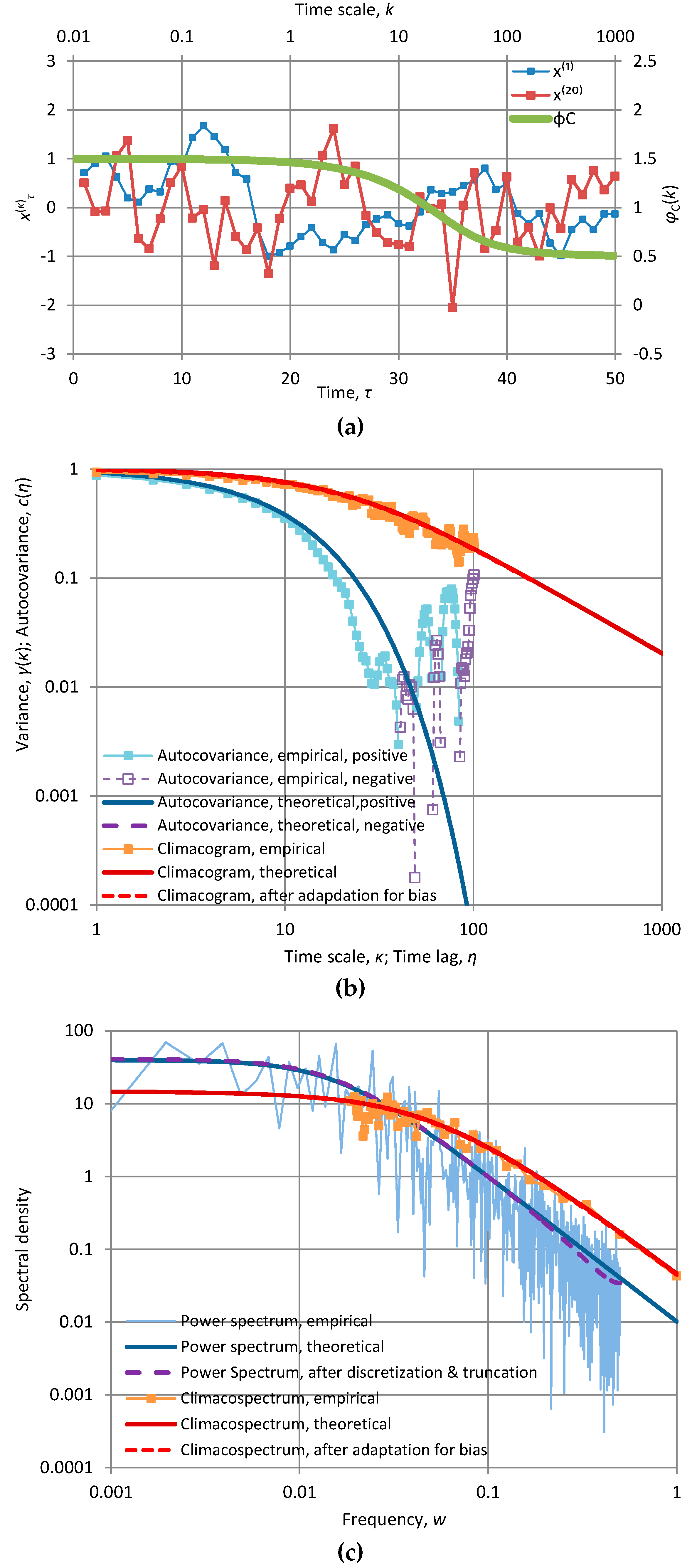
Appendix A.2.2. FHK Process with Cauchy-Type Climacogram (FHK-C)
General description of the FHK process with Cauchy-type climacogram (FHK-C) is given in Section 3.2 and its detailed mathematical expressions and asymptotic processes are given in Table A2.
Table A2.
Mathematical expressions of the second order characteristics of the FHK process with Cauchy-type climacogram (FHK-C) and their asymptotic properties.
Table A2.
Mathematical expressions of the second order characteristics of the FHK process with Cauchy-type climacogram (FHK-C) and their asymptotic properties.
| Characteristic | Mathematical Expression | Local Asymptotic Properties | Global Asymptotic Properties | Equation |
|---|---|---|---|---|
| Climacogram | (A75) | |||
| Climacospectrum | (A76) | |||
| Entropy production | (A77) | |||
| Autocovariance function | 0 | (A78) | ||
| Power spectrum | Analytical expression not possible except in special cases; numerical solution easily derived from (10) | (A79) |
This model is very rich as it covers the entire admissible range, by appropriate choice of the smoothness parameter (0 < M ≤ 1) and persistence parameter (0 ≤ H < 1). It represents smooth processes (if M > ½), rough processes (if M < ½), persistent processes (if H > ½) and antipersistent processes (if H < ½). For M = H = ½ it becomes a neutral process, practically identical to Markov.
The FHK process can even produce near pink (1/f) noise if M = 1 − H ≈ 0, which is associated with maximal entropy production for large scales and minimal for small scales. In this case the quantity is close to 1 and the following approximation holds:
This can be verified by observing that for x close to 1 the quantities ln x and are close to each other, differing only by a factor of O[x − 1]3.
For M = H ≈ 0, we have minimal entropy production for all scales. In this case:
This can be verified by observing that for x close to 1 the logarithms of the two quantities differ only by a factor of H O[x − 1]2. We note that both (A80) and (A81) violate the condition for physical consistency (finite variance).
A set of applications of the FHK-C are depicted in detail in Figure A3, Figure A4, Figure A5, Figure A6 and Figure A7, which are also discussed in Section 3.2. It is observed that the SMA generation scheme performs almost perfectly even in the most extreme cases and that the climacogram-based characteristics perform better than the autocorrelation-based ones.
![Entropy 19 00581 g010]()
![Entropy 19 00581 g011]()
![Entropy 19 00581 g012]()
![Entropy 19 00581 g013]()
![Entropy 19 00581 g014]()
Figure A3.
Characteristic graphs as in Figure A2 but for a time series generated by the FHK-C model with γ(1) = 1, α = 10 and H = M = 0.97.
Figure A3.
Characteristic graphs as in Figure A2 but for a time series generated by the FHK-C model with γ(1) = 1, α = 10 and H = M = 0.97.

Figure A4.
Characteristic graphs as in Figure A2 but for a time series generated by the FHK-C model with γ(1) = 1, α = 10, and H = M = 0.05.
Figure A4.
Characteristic graphs as in Figure A2 but for a time series generated by the FHK-C model with γ(1) = 1, α = 10, and H = M = 0.05.

Figure A5.
Characteristic graphs as in Figure A2 but for a time series generated by the FHK-C model with γ(1) = 1, α = 10, H = 0.99 and M = 0.01 (close to “pink noise”).
Figure A5.
Characteristic graphs as in Figure A2 but for a time series generated by the FHK-C model with γ(1) = 1, α = 10, H = 0.99 and M = 0.01 (close to “pink noise”).

Figure A6.
Characteristic graphs as in Figure A2 but for a time series generated by the FHK-C model with γ(1) = 1, α = 10, H = 0.01 and M = 0.99.
Figure A6.
Characteristic graphs as in Figure A2 but for a time series generated by the FHK-C model with γ(1) = 1, α = 10, H = 0.01 and M = 0.99.

Figure A7.
Characteristic graphs as in Figure A2 but for a time series generated by the FHK-C model with γ(1) = 1, α = 100 and H = M = 0.75.
Figure A7.
Characteristic graphs as in Figure A2 but for a time series generated by the FHK-C model with γ(1) = 1, α = 100 and H = M = 0.75.
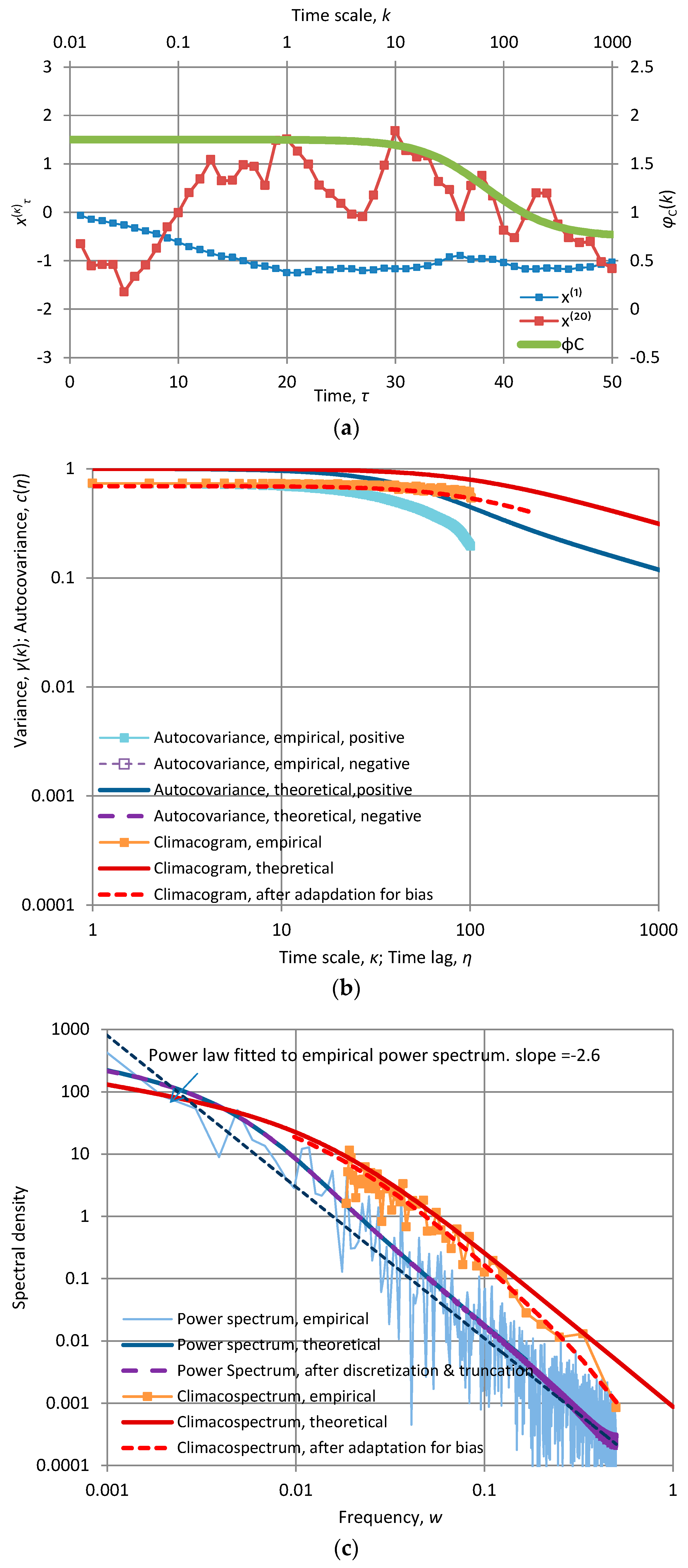
Appendix A.2.3. FHK Process with Dagum-Type Climacogram (FHK-D)
The FHK process with Dagum-type climacogram (FHK-D) has expressions for its second order characteristics different from those of the Cauchy-type climacogram (see Table A3). However, the behaviour of the two models, as well as the meaning and ranges of parameters, are the same. For M = 1 − H the two models become precisely identical. The model is particularly useful in combination with the FHK-C model as shown below.
Table A3.
Mathematical expressions of the second order characteristics of the FHK process with Dagum-type climacogram (FHK-D) and their asymptotic properties.
Table A3.
Mathematical expressions of the second order characteristics of the FHK process with Dagum-type climacogram (FHK-D) and their asymptotic properties.
| Characteristic | Mathematical Expression | Local Asymptotic Properties | Global Asymptotic Properties | Equation |
|---|---|---|---|---|
| Climacogram | (A82) | |||
| Climacospectrum | (A83) | |||
| Entropy production | (A84) | |||
| Autocovariance function | 0 | (A85) | ||
| Power spectrum | Analytical expression not possible except in special cases; numerical solution easily derived from (10) | (A86) |
Appendix A.2.4. FHK Process with Climacogram Equal to the Sum of a Cauchy and a Dagum Climacograms (FHK-CD)
By summing a Cauchy-type climacogram with M = 1 and a Dagum-type climacogram with H = 0 we get the FHK-CD model whose second-order characteristics are shown in Table A4. This is a convenient model, in which the first additive term determines merely the persistence of the process and the second one the smoothness of the process. It is more convenient that its constituents as most of mathematical expressions are simpler; in particular, it results in an explicit relationship of the power spectrum, which however is not very simple. In addition, it is more flexible and richer than its constituents, as it contains two couples of scale parameters; however, if parsimony is sought, then it can take the same number of parameters as each of the constituents by setting α1 = α2 and λ1 = λ2 (it is reminded that one λ and one α are absolutely minimal requirements of parameters).
An application of the model based on real measurements of turbulent velocities is contained in Section 3.4.
Another option, of the same type, not studied in detail here, would be to sum a Cauchy-type climacogram with M = ½ and a Dagum-type climacogram with H = ½. The climacogram of the thus formed model is:
The model (A87), however, can only produce rough persistent processes with and . Indeed, it is easily shown that in this case ) and . The turbulent velocity case, studied in Section 3.4, belongs to this domain and thus the model (A87) could also be used as an alternative.
Table A4.
Mathematical expressions of the second order characteristics of the FHK process formed as the sum of a Cauchy and a Dagum process (FHK-CD) dealing separately with persistence and smoothness, respectively, and their asymptotic properties.
Table A4.
Mathematical expressions of the second order characteristics of the FHK process formed as the sum of a Cauchy and a Dagum process (FHK-CD) dealing separately with persistence and smoothness, respectively, and their asymptotic properties.
| Characteristic | Mathematical Expression | Local Asymptotic Properties | Global Asymptotic Properties | Equation |
|---|---|---|---|---|
| Climacogram | (A88) | |||
| Climacospectrum | (A89) | |||
| Entropy production | (A90) | |||
| Autocovariance function | 0 | (A91) | ||
| Power spectrum | Analytical expression too complex, derived from (10) | (A92) |
Appendix A.2.5. Smooth Process with Generalized Exponential-Type Autocovariance (SE)
By generalizing the power spectrum of a Markov process, as seen in Table A5, we can obtain a smooth processes (the smooth exponential process—SE). Generalization is made by introducing an integral parameter n = 0, 1, 2, …, where the value n = 0 results precisely in a Markov process. A notable characteristic of the process is that it corresponds to the absolute maximum of entropy production for small scales.
Table A5.
Mathematical expressions of the second order characteristics of the SE process and their asymptotic properties.
Table A5.
Mathematical expressions of the second order characteristics of the SE process and their asymptotic properties.
| Characteristic | Mathematical Expression | Local Asymptotic Properties | Global Asymptotic Properties | Equation |
|---|---|---|---|---|
| Climacogram | where n = 0, 1, 2, …, is a polynomial and a coefficient, both determined using (23); the first five are: | (A93) | ||
| Climacospectrum | (A94) | |||
| Entropy production | where are coefficients as above and are polynomials determined using (39); the first five are: | (A95) | ||
| Autocovariance function | where is a polynomial determined by the power spectrum (see below) using (22); the first five are: | 0 | (A96) | |
| Power spectrum | (A97) |
Appendix A.2.6. Antipersistent Process with Generalized Exponential-Type Autocovariance (AE)
This is again a generalization of the Markov process by introducing an integral parameter n = 0, 1, 2, …, where the value n = 0 results precisely in a Markov process. Its characteristics are shown in Table A6. The process is antipersistent and its most notable characteristic is that it corresponds to the absolute minimum of entropy production for large scales. An application of the process is shown in Figure A8 for n = 2; the hole in the function φC(k) for moderate k is a characteristic of this process.
![Entropy 19 00581 g015]()
Table A6.
Mathematical expressions of the second order characteristics of the AE process and their asymptotic properties.
Table A6.
Mathematical expressions of the second order characteristics of the AE process and their asymptotic properties.
| Characteristic | Mathematical Expression | Local Asymptotic Properties | Global Asymptotic Properties | Equation |
|---|---|---|---|---|
| Climacogram | where n = 0, 1, 2…, while for n > 0 is a polynomial determined using (23); the first four are: | (A98) | ||
| Climacospectrum | (A99) | |||
| Entropy production | where , while for n > 0 are polynomials determined using (39); the first four are: | (A100) | ||
| Autocovariance function | where is a polynomial determined by the power spectrum (see below) using (22); the first five are:1 | 0 | (A101) | |
| Power spectrum | (A102) |
Figure A8.
Characteristic graphs as in Figure A2 but for a time series generated by the AE model with γ(1) = 1, α = 10 and n = 2.
Figure A8.
Characteristic graphs as in Figure A2 but for a time series generated by the AE model with γ(1) = 1, α = 10 and n = 2.

Appendix A.2.7. Generalized Planck Model (GP)
The generalized Planck (GP) model is obtained by a generalization of Planck’s law of black-body radiation, introducing an integral parameter n = 0, 1, 2, …, where the value n = 1 corresponds to Planck’s law precisely. The process, whose detailed equations are given in Table A7, is simultaneously extremely smooth (φC(0) = 2) and extremely antipersistent (φC(∞) = 0). An application for n = 1 is depicted in Figure A9.
![Entropy 19 00581 g016]()
Table A7.
Mathematical expressions of the second order characteristics of the Generalized Planck (GP) process and their asymptotic properties.
Table A7.
Mathematical expressions of the second order characteristics of the Generalized Planck (GP) process and their asymptotic properties.
| Characteristic | Mathematical Expression | Local Asymptotic Properties | Global Asymptotic Properties | Equation |
|---|---|---|---|---|
| Climacogram | where n = 0, 1, 2, …, is a function determined using (23) the first three are: | n = 0 n > 0 | (A103) | |
| Climacospectrum | n = 0 n > 0 | (A104) | ||
| Entropy production | φ(k) is determined from (39); the first three terms are: | φ(0) = 1 φC(0) = 2 | φ(∞) = φC(∞) = 1/2, n = 0 φ(∞) = φC(∞) = 0, n > 0 | (A105) |
| Autocovariance function | where is a function determined from (22); the first three are: | 0 | (A106) | |
| Power spectrum | where cn is a normalizing constant making the area of the power spectrum ; the first three are c0 = 24, c1 = 240, c2 = 504 | (A107) | ||
Figure A9.
Characteristic graphs as in Figure A2 but for a time series generated by the GP model with γ(1) = 1, α = 10 and n = 1.
Figure A9.
Characteristic graphs as in Figure A2 but for a time series generated by the GP model with γ(1) = 1, α = 10 and n = 1.
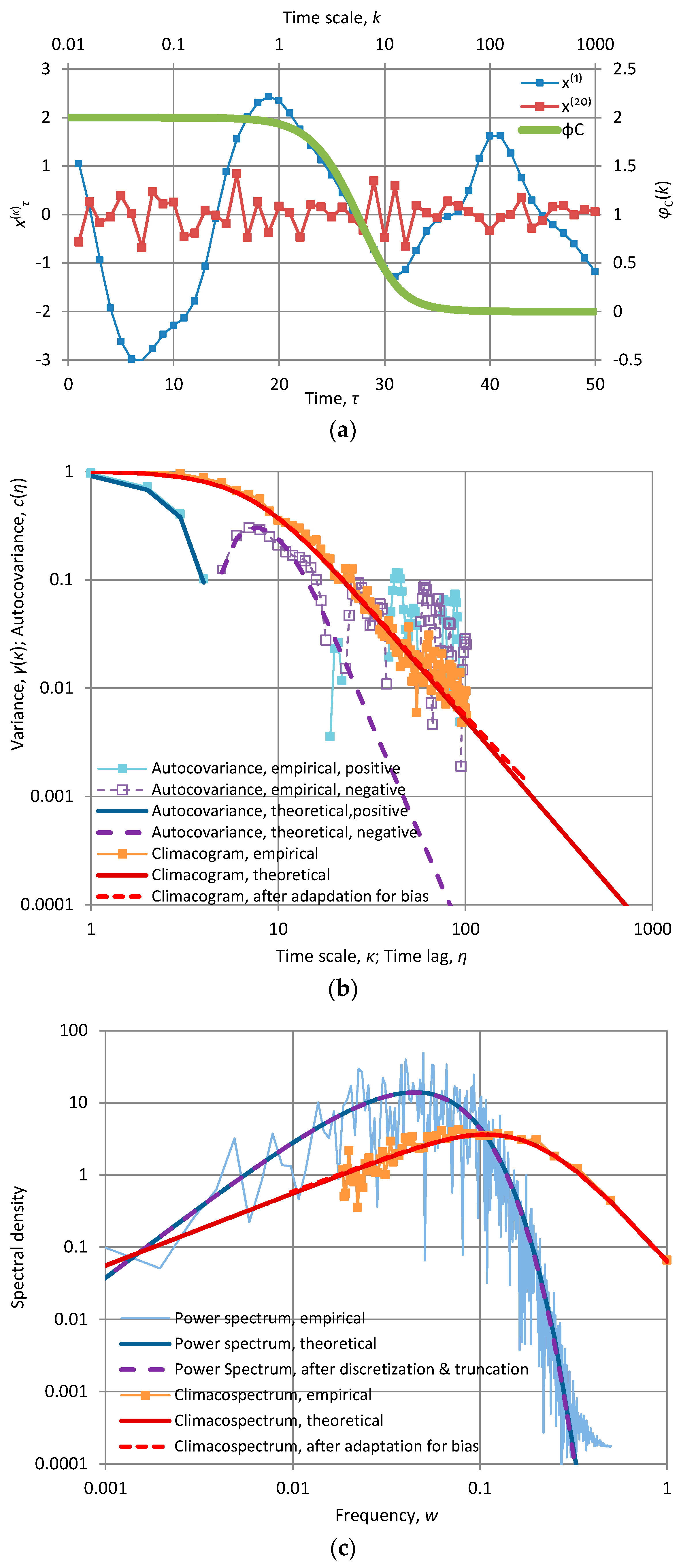
Appendix A.2.8. Harmonic Oscillation Treated as a Stochastic Process
A harmonic oscillation, here expressed as
is very easily modelled as a deterministic process but, when it is superimposed to a stochastic process, the resulting process is a stochastic process, too. Obviously the second-order characteristics of this composite process are affected by periodic components and therefore we need to know which equations should be superimposed to those of the stochastic component (see also [40,41]). These equations are given in Table A8. Remarkably, the climacogram retains information about the phase (2πb/T) of the process (through the spikes appearing at , m ∈ N0, which depend on the phase). Note that this information is completely lost in the autocovariance function and the power spectrum.
An application is depicted in Figure A10. The example process is the average of a FHK with H = M = 0.8 and a harmonic oscillation. It is difficult to identify the presence of the oscillation from visual inspection of the time series, but the detailed graph of any of the second-order characteristics, plotted in Figure A10, captures the periodic behaviour. Note that for the application, the generation was done by the SMA model for the entire (composite) process and not by separating the generation of the stochastic and the deterministic component. This is an indication of the flexibility and generality of the generation algorithm.
![Entropy 19 00581 g017]()
Table A8.
Mathematical expressions of the second order characteristics of a harmonic oscillation treated as a stochastic process and their asymptotic properties.
Table A8.
Mathematical expressions of the second order characteristics of a harmonic oscillation treated as a stochastic process and their asymptotic properties.
| Characteristic | Mathematical Expression | Local Asymptotic Properties | Global Asymptotic Properties | Equation |
|---|---|---|---|---|
| Climacogram | where T is the period, m ∈ N0 and the harmonic oscillation is described by , 0 ≤ b ≤ T | (A109) | ||
| Climacospectrum | does not converge as k → | (A110) | ||
| Entropy production | (for ) | and do not converge as k → | (A111) | |
| Autocovariance function | 0 | does not converge as k → | (A112) | |
| Power spectrum | (not applicable) | (A113) | ||
Figure A10.
Characteristic graphs as in Figure A2 but for a time series generated by the FHK-C model with λ = 1, α = 10, and H = M = 0.8 in which a harmonic oscillation with T = 5α = 50 is superimposed.
Figure A10.
Characteristic graphs as in Figure A2 but for a time series generated by the FHK-C model with λ = 1, α = 10, and H = M = 0.8 in which a harmonic oscillation with T = 5α = 50 is superimposed.
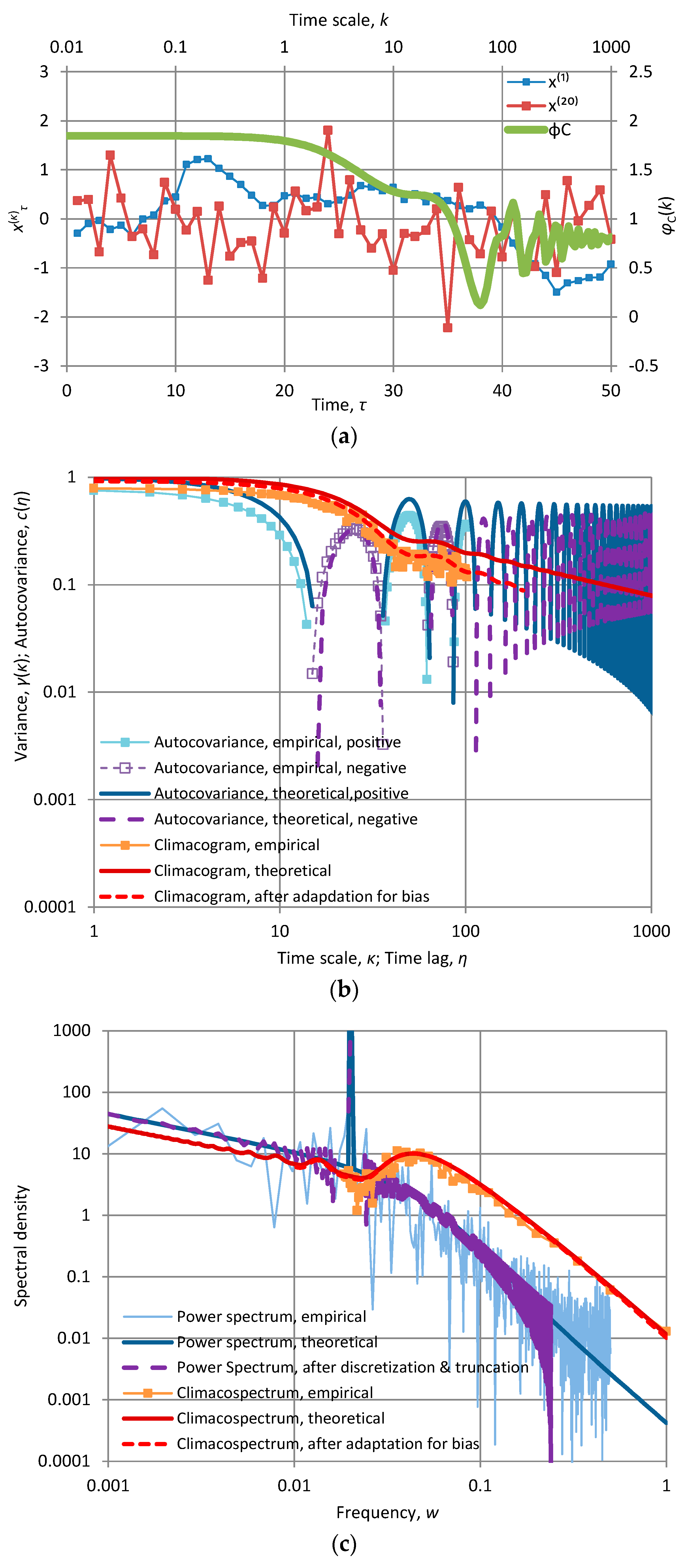
References
- Boltzmann, L. Über die Beziehung zwischen dem zweiten Hauptsatze der mechanischen Wärmetheorie und der Wahrscheinlichkeitsrechnung respektive den Sätzen über das Wärmegleichgewicht. Wien. Ber. 1877, 76, 373–435. (In German) [Google Scholar]
- Shannon, C.E. The mathematical theory of communication. Bell Syst. Tech. J. 1948, 27, 379–423. [Google Scholar] [CrossRef]
- Jaynes, E.T. Information theory and statistical mechanics. Phys. Rev. 1957, 106, 620–630. [Google Scholar] [CrossRef]
- Sonuga, J.O. Principle of maximum entropy in hydrologic frequency analysis. J. Hydrol. 1972, 17, 177–191. [Google Scholar] [CrossRef]
- Jackson, D.R.; Aron, G. Parameter estimation in hydrology: The state of the art. J. Am. Water Resour. Assoc. 1971, 7, 457–472. [Google Scholar] [CrossRef]
- Singh, V.P.; Fiorentino, M. A Historical Perspective of Entropy Applications in Water Resources. In Entropy and Energy Dissipation in Water Resources; Singh, V.P., Fiorentino, M., Eds.; Springer: Dordrecht, The Netherlands, 1992. [Google Scholar]
- Singh, V.P. The use of entropy in hydrology and water resources. Hydrol. Process. 1997, 11, 587–626. [Google Scholar] [CrossRef]
- Singh, V.P. Hydrologic synthesis using entropy theory: review. J. Hydrol. Eng. 2011, 16, 421–433. [Google Scholar] [CrossRef]
- Singh, V.P.; Cui, H. Entropy Theory for Groundwater Modeling. Available online: http://www.aggs.in/Issues/JGWR-2015101.pdf (accessed on 24 October 2017).
- Singh, V.P.; Cui, H. Entropy theory for streamflow forecasting. Environ. Process. 2015, 2, 449–460. [Google Scholar] [CrossRef]
- Singh, V.P. Entropy theory. In Handbook of Applied Hydrology, 2nd ed.; Singh, V.P., Ed.; McGraw Hill: New York, NY, USA, 2017. [Google Scholar]
- Porporato, A.; Rigby, J.R.; Daly, E. Irreversibility and fluctuation theorem in stationary time series. Phys. Rev. Lett. 2007, 98, 94101. [Google Scholar] [CrossRef] [PubMed]
- Kondepudi, D.; Prigogine, I. Modern Thermodynamics; Wiley: Chichester, UK, 1998. [Google Scholar]
- Pujol, T.; Llebot, J.E. Extremal principle of entropy production in the climate system. Q. J. R. Meteorol. Soc. 1999, 125, 79–90. [Google Scholar] [CrossRef]
- Ozawa, H.; Ohmura, A.; Lorenz, R.D.; Pujol, T. The second law of thermodynamics and the global climate system: A review of the maximum entropy production principle. Rev. Geophys. 2003, 41. [Google Scholar] [CrossRef]
- Prigogine, I. Moderation et transformations irreversibles des systemes ouverts. Bull. Classe Sci. Acad. R. Belg. 1945, 31, 600–606. [Google Scholar]
- Ziegler, H. Progress in Solid Mechanics; Sneddon, I.N., Hill, R., Eds.; North-Holland: Amsterdam, The Netherlands, 1963; Volume 4. [Google Scholar]
- Martyushev, L.M.; Seleznev, V.D. Maximum entropy production principle in physics, chemistry and biology. Phys. Rep. 2006, 426. [Google Scholar] [CrossRef]
- Niven, R. Entropy production extremum principles. In Handbook of Applied Hydrology, 2nd ed.; Singh, V.P., Ed.; McGraw Hill: New York, NY, USA, 2017. [Google Scholar]
- Koutsoyiannis, D. HESS Opinions: A random walk on water. Hydrol. Earth Syst. Sci. 2010, 14, 585–601. [Google Scholar] [CrossRef]
- Montanari, A.; Koutsoyiannis, D. A blueprint for process-based modeling of uncertain hydrological systems. Water Resour. Res. 2012, 48, W09555. [Google Scholar] [CrossRef]
- Koutsoyiannis, D. Hurst-Kolmogorov dynamics as a result of extremal entropy production. Phys. A Stat. Mech. Appl. 2011, 390, 1424–1432. [Google Scholar] [CrossRef]
- Hemelrijk, J. Underlining random variables. Stat. Neerl. 1966, 20. [Google Scholar] [CrossRef]
- Koutsoyiannis, D. Generic and parsimonious stochastic modelling for hydrology and beyond. Hydrol. Sci. J. 2016, 61, 225–244. [Google Scholar] [CrossRef]
- Koutsoyiannis, D.; Montanari, A. Negligent killing of scientific concepts: The stationarity case. Hydrol. Sci. J. 2015, 60, 1174–1183. [Google Scholar] [CrossRef]
- Kolmogorov, A.N. A simplified proof of the Birkhoff-Khinchin ergodic theorem. Uspekhi Mat. Nauk 1938, 5, 52–56. [Google Scholar]
- Papoulis, A. Probability, Random Variables and Stochastic Processes, 3rd ed.; McGraw-Hill: New York, NY, USA, 1991. [Google Scholar]
- Dimitriadis, P.; Koutsoyiannis, D. Climacogram versus autocovariance and power spectrum in stochastic modelling for Markovian and Hurst–Kolmogorov processes. Stoch. Environ. Res. Risk Assess. 2015, 29, 1649–1669. [Google Scholar] [CrossRef]
- Koutsoyiannis, D. Physics of uncertainty, the Gibbs paradox and indistinguishable particles. Stud. Hist. Philos. Mod. Phys. 2013, 44, 480–489. [Google Scholar] [CrossRef]
- Koutsoyiannis, D. Entropy: from thermodynamics to hydrology. Entropy 2014, 16, 1287–1314. [Google Scholar] [CrossRef]
- Koutsoyiannis, D.; Dimitriadis, P.; Lombardo, F.; Stevens, S. From fractals to stochastics: Seeking theoretical consistency in analysis of geophysical data. In Advances in Nonlinear Geosciences; Tsonis, A., Ed.; Springer: New York, NY, USA, 2018. [Google Scholar]
- Dechant, A.; Lutz, E. Wiener-Khinchin theorem for nonstationary scale-invariant processes. Phys. Rev. Lett. 2015, 115, 80603. [Google Scholar] [CrossRef] [PubMed]
- Mandelbrot, B. Gaussian Self-Affinity and Fractals: Globality, the Earth, 1/f Noise, and R/S (Vol. 8); Springer: New York, NY, USA, 2002. [Google Scholar]
- Kitanidis, P.K. Geostatistics. In Handbook of Hydrology; Maidment, D.R., Ed.; McGraw-Hill: New York, NY, USA, 1993. [Google Scholar]
- Gaetan, C.; Guyon, X. Spatial Statistics and Modeling; Springer: New York, NY, USA, 2010. [Google Scholar]
- Clark, I. Statistics or geostatistics? Sampling error or nugget effect? J. South. Afr. Inst. Min. Metall. 2010, 110, 307–312. [Google Scholar]
- Gneiting, T.; Schlather, M. Stochastic models that separate fractal dimension and the Hurst effect. SIAM Rev. 2004, 46, 269–282. [Google Scholar] [CrossRef]
- Keshner, M.S. 1/f noise. Proc. IEEE 1982, 70, 212–218. [Google Scholar] [CrossRef]
- Wornell, G.W. Wavelet-based representations for the 1/f family of fractal processes. Proc. IEEE 1993, 81, 1428–1450. [Google Scholar] [CrossRef]
- Markonis, Y.; Koutsoyiannis, D. Climatic variability over time scales spanning nine orders of magnitude: Connecting Milankovitch cycles with Hurst–Kolmogorov dynamics. Surv. Geophys. 2013, 34, 181–207. [Google Scholar] [CrossRef]
- Pappas, C.; Mahecha, M.D.; Frank, D.C.; Babst, F.; Koutsoyiannis, D. Ecosystem functioning is enveloped by hydrometeorological variability. Nat. Ecol. Evol. 2017, 1, 1263–1270. [Google Scholar] [CrossRef] [PubMed]
- Kang, H.S.; Chester, S.; Meneveau, C. Decaying turbulence in an active-grid-generated flow and comparisons with large-eddy simulation. J. Fluid Mech. 2003, 480, 129–160. [Google Scholar] [CrossRef]
- Dimitriadis, P.; Koutsoyiannis, D. Stochastic synthesis approximating any process dependence and distribution. Stoch. Environ. Res. Risk Assess. 2017. submitted. [Google Scholar]
- Jaynes, E.T. Probability Theory: The Logic of Science; Cambridge University Press: Cambridge, UK, 2003; p. 728. [Google Scholar]
- Swendsen, R.H. How physicists disagree on the meaning of entropy. Am. J. Phys. 2011, 79, 342–348. [Google Scholar] [CrossRef]
- Stein, M.L. Interpolation of Spatial Data; Springer: New York, NY, USA, 1999. [Google Scholar]
- Beran, J. Statistics for Long-Memory Processes; Chapman and Hall: New York, NY, USA, 1994. [Google Scholar]
- Taqqu, M.S. Fractional Brownian motion and long-range dependence. In Theory and Applications of Long-Range Dependence; Doukhan, P., Oppenheim, G., Taqqu, M.S., Eds.; Birkhäuser: Boston, MA, USA, 2003. [Google Scholar]
Figure 1.
Explanatory sketch for a stochastic process in continuous time and in discrete time. Note that the graphs display a realization of the process (it is impossible to display the process as such) while the notation is for the process per se (adapted from [24]).
Figure 1.
Explanatory sketch for a stochastic process in continuous time and in discrete time. Note that the graphs display a realization of the process (it is impossible to display the process as such) while the notation is for the process per se (adapted from [24]).

Figure 2.
Bounds of asymptotic values of CEPLT, φC(0) and φC(∞), and corresponding bounds of the log-log slopes of power spectrum and climacospectrum The “green square” represents the admissible region (note that s# can, by exception, take on values out of the square when φC(0) = 2 or φC(∞) = 0). The reasons why a process out of the square would be impossible or inconsistent are also marked. The lines φC(0) = 3/2 and φC(∞) = 1/2 represent neutrality and support the classification of stochastic processes into the indicated four categories (smaller squares within the “green square”).

Figure 3.
A power type variogram model with “nugget effect” (green dotted line), with equation vE(h) = 0.83 (h + 0.05)0.03 (corresponding to a “nugget” value v(0) = 0.83 (0.05)0.03 = 0.76) and its replacement with a FHK-C model with H = 0.75 and M = 0.2.
Figure 3.
A power type variogram model with “nugget effect” (green dotted line), with equation vE(h) = 0.83 (h + 0.05)0.03 (corresponding to a “nugget” value v(0) = 0.83 (0.05)0.03 = 0.76) and its replacement with a FHK-C model with H = 0.75 and M = 0.2.
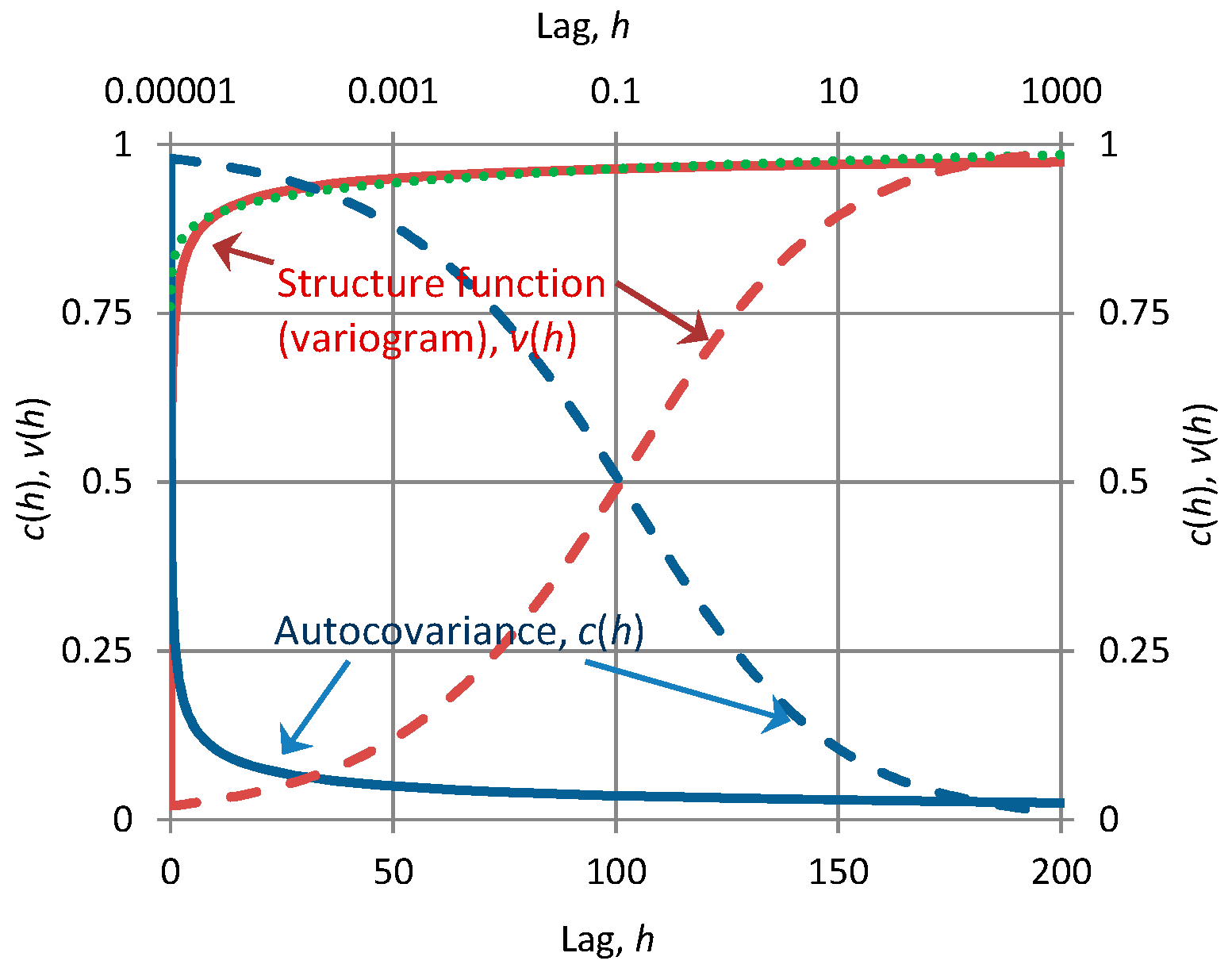
Figure 4.
The first fifty terms at time scales k = 1 and 20 of time series produced by various models, along with “stamps” of the models (green lines plotted with respect to the secondary axes) represented by the CEPLT, φC(k). The different models are (a) Markov; (b) FHK, with CEPLT close to the absolute maximum (H = M = 0.97); (c) FHK, with CEPLT close to the absolute minimum (H = M = 0.05); (d) FHK, with CEPLT close to the absolute maximum for large scales (H = 0.99) and close to the absolute minimum for small scales (M = 0.01); (e) GP with n = 1 (blackbody spectrum) with CEPLT equal to the absolute minimum (0) for large scales and to the absolute maximum (2) for small scales; (f) Approximation of (e) by FHK (H = 0.01, M = 0.99, also using the same initial sequence of random numbers as in (e) to visualize similarity); (g) AE with n = 2; (h) average of a FHK with H = M = 0.8 and a harmonic oscillation with T = 5α = 50. In all cases the discretization time scale is D = 1, the characteristic time scale a = 10, and the characteristic variance scale λ is chosen so that for time scale D, γ(D) = 1. The mean is 0 in all cases and the marginal distribution is normal. The FHK is implemented using the Cauchy-type climacogram.

Figure 5.
Ranges of asymptotic values for each of the most important second order functions of the examined processes. Wide light blue lines/boxes represent global properties (k, h → ∞, w → 0) while narrow dark red lines/boxes represent local properties (k, h → 0, w → ∞). Markov: Markov process; FHK: filtered Hurst-Kolmogorov process in any of the three forms; SE: smooth process with generalized exponential-type autocovariance; AE: antipersistent process with generalized exponential-type autocovariance; GP: generalized Planck. Note that the Markov process is identical with the SE and PE for n = 0.

Figure 6.
Envelopes of ranges of asymptotic values for each of the most important second order functions for all examined processes.
Figure 6.
Envelopes of ranges of asymptotic values for each of the most important second order functions for all examined processes.
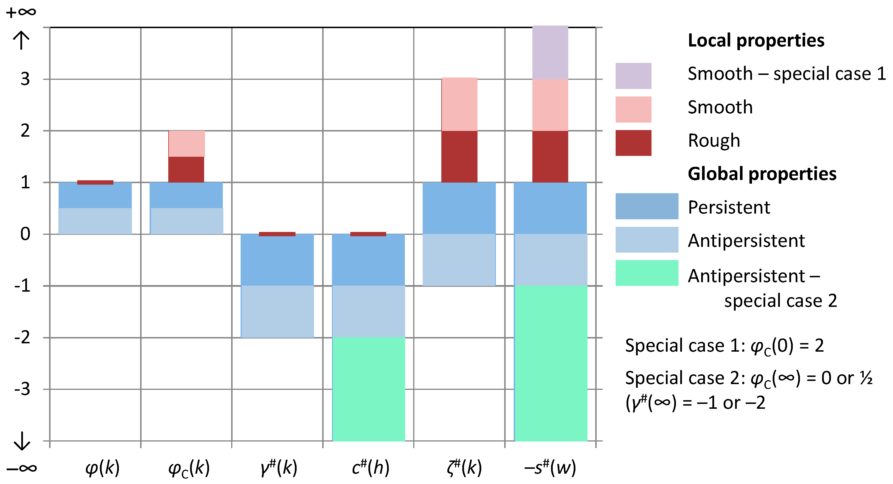
Figure 7.
Characteristic graphs of the turbulent velocity time series: (a) plot of the first fifty terms of the time series at time scales κ = 1, 20, 400 and 8000, along with the “stamp” φC(k) of the fitted model (green line plotted with respect to the secondary axes); (b) empirical and fitted theoretical climacogram; (c) empirical and fitted theoretical climacospectrum.

Table 1.
Definition of main characteristics and notations for a stochastic process in continuous time; see Figure 1 for clarification.
Table 1.
Definition of main characteristics and notations for a stochastic process in continuous time; see Figure 1 for clarification.
| Name of Quantity or Characteristic | Symbol and Definition | Remarks | Equation |
|---|---|---|---|
| Stochastic process of interest | x(t) | Assumed stationary | |
| Time, continuous | t | Dimensional quantity | |
| Cumulative process | Nonstationary | (3) | |
| Variance, instantaneous | γ0 ≔ Var[x(t)] | Constant (not a function of t) | (4) |
| Cumulative climacogram | Γ(t) ≔ Var[X(t)] | A function of t, Γ(0) = 0 | (5) |
| Climacogram | γ(k) ≔ Var[(1/k)(X(t + k) − X(t))] = Var[X(k)/k] = Γ(k)/k2 | Not a function of t, γ(0) = γ0 | (6) |
| Time scale, continuous | k | Units of time | |
| Autocovariance function | c(h) := Cov[x(t), x(t + h)] | c(0) = γ0 | (7) |
| Time lag, continuous | h | Units of time | |
| Structure function (or semivariogram or variogram) | [x(t) − x(t + h)] | (8) | |
| Climacostructure function | ξ(k) ≔ γ0 − γ(k) | (9) | |
| Power spectrum (or spectral density) | (10) | ||
| Frequency, continuous | w = 1/k | Units of inverse time | (11) |
Table 2.
Definition of main characteristics and notations for a stochastic process in discrete time and their relationship with those in continuous time; see Figure 1 for clarification.
Table 2.
Definition of main characteristics and notations for a stochastic process in discrete time and their relationship with those in continuous time; see Figure 1 for clarification.
| Name of Quantity or Characteristic | Symbol and Definition | Remarks | Equation |
|---|---|---|---|
| Stochastic process, discrete time | (12) | ||
| Time unit = discretization time step | D | Time step or length of time window of averaging | |
| Time, discrete | τ := t/D | Dimensionless quantity, integer | (13) |
| Characteristic variance | Var[ ] = γ(D) | (14) | |
| Climacogram | = γ(D) | (15) | |
| Time scale, discrete | κ := k/D | Dimensionless quantity | (16) |
| Autocovariance function | ≔ Cov[] | ||
| Time lag, discrete | η := h/D | Dimensionless quantity | (17) |
| Structure function | (18) | ||
| Power spectrum | (19) | ||
| Frequency, discrete | ω := wD = 1/κ | Dimensionless quantity | (20) |
Note: In time-related quantities, Latin letters denote dimensional quantities and Greek letters dimensionless ones. The Latin i, j, l may also be used as integers to denote quantities τ, η, κ, depending on the context.
Table 3.
Relationships between several characteristics of a process in continuous and discrete time.
Table 3.
Relationships between several characteristics of a process in continuous and discrete time.
| Related Characteristics | Direct Relationship | Inverse Relationship | Equation |
|---|---|---|---|
| (21) | |||
| (22) | |||
| (23) | |||
| (24) | |||
| ξ(k) ≔ γ0 − γ(k) | γ(k) = ξ(∞) − ξ(k) ( | (25) | |
| (26) | |||
Alternatively, where, in recursive mode, with , | (27) | ||
| (28) | |||
| (29) |
Table 4.
Models that can perform in each of the specified extremal or neutral cases of smoothness and persistence.
Table 4.
Models that can perform in each of the specified extremal or neutral cases of smoothness and persistence.
| Persistence | Smoothness | ||
|---|---|---|---|
| Maximal Roughness | Neutral Smoothness | Maximal Smoothness | |
| Maximal Persistence, | ~FHK | ~FHK | ~FHK |
| Neutral Persistence | ~FHK | Markov, FHK | SE, GP, FHK |
| Maximal Antipersistence | ~FHK | AE, FHK | GP, FHK |
Note: the symbol ‘~’ indicates that the model can perform in close approximation but not precisely.
© 2017 by the author. Licensee MDPI, Basel, Switzerland. This article is an open access article distributed under the terms and conditions of the Creative Commons Attribution (CC BY) license (http://creativecommons.org/licenses/by/4.0/).
Share and Cite
MDPI and ACS Style
Koutsoyiannis, D. Entropy Production in Stochastics. Entropy 2017, 19, 581. https://doi.org/10.3390/e19110581
AMA Style
Koutsoyiannis D. Entropy Production in Stochastics. Entropy. 2017; 19(11):581. https://doi.org/10.3390/e19110581
Chicago/Turabian StyleKoutsoyiannis, Demetris. 2017. "Entropy Production in Stochastics" Entropy 19, no. 11: 581. https://doi.org/10.3390/e19110581
Note that from the first issue of 2016, this journal uses article numbers instead of page numbers. See further details here.