A Connection Entropy Approach to Water Resources Vulnerability Analysis in a Changing Environment


1
School of Civil Engineering and Environmental Engineering, Anhui Xinhua University, Hefei 230088, China
2
Institute of Safety and Environmental Assessment, Anhui Xinhua University, Hefei 230088, China
3
School of Civil Engineering, Hefei University of Technology, Hefei 230009, China
4
Ministry of Education Key Lab of Water and Sand Science, School of Environment, Beijing Normal University, Beijing 100875, China
*
Author to whom correspondence should be addressed.
Entropy 2017, 19(11), 591; https://doi.org/10.3390/e19110591
Submission received: 5 September 2017
/
Revised: 26 October 2017
/
Accepted: 1 November 2017
/
Published: 6 November 2017
(This article belongs to the Special Issue Entropy Applications in Environmental and Water Engineering)
Abstract
:This paper establishes a water resources vulnerability framework based on sensitivity, natural resilience and artificial adaptation, through the analyses of the four states of the water system and its accompanying transformation processes. Furthermore, it proposes an analysis method for water resources vulnerability based on connection entropy, which extends the concept of contact entropy. An example is given of the water resources vulnerability in Anhui Province of China, which analysis illustrates that, overall, vulnerability levels fluctuated and showed apparent improvement trends from 2001 to 2015. Some suggestions are also provided for the improvement of the level of water resources vulnerability in Anhui Province, considering the viewpoint of the vulnerability index.
1. Introduction
The concept of vulnerability has its roots in geography and natural hazards research. Moreover, the original concept is the degree to which a system is likely to experience harm because of exposure to a hazard [1,2]. Vulnerability is now considered a central concept in a variety of other research contexts including anthropology, sociology, economics, aerography, ecology, management and sustainability science [3]. There are two key research perspectives in water resources vulnerability: a major role key research perspective is vulnerability of single purpose water systems, such as surface water vulnerability, groundwater vulnerability, and vulnerability of the drinking water supplies, etc. Padowski and Gorelick [4] presented a global analysis of urban water supply vulnerability in 70 surface water-supplied cities in a baseline (2010) condition and a future scenario (2040), which considered increased demand from urban population growth and projected agricultural demand under normal climate conditions, but did not account for climate change. Allouchea et al. [5] assessed groundwater vulnerability to contamination from anthropogenic activities and sea water intrusion based on a more robust “global risk index”, and the DRASTIC and GALDIT parametric methods were then linked to a novel land use index. Khakhar et al. [6] derived the intrinsic vulnerability of groundwater against contamination using the GIS platform, and applied DRASTIC model for Ahmedabad district in Gujarat (India), that also contributes to validating the existence of higher concentrations of contaminants/indicators with respect to groundwater vulnerability status in the study area. Rushforth and Ruddell [7] spatially mapped and analyzed the Water Footprint of Flagstaff (AZ, USA), using a county-level database of the U.S. hydro-economy, NWED, which can empower city managers to operationalize a city’s water footprint information to reduce vulnerability and increase resilience. Martinez et al. [8] assessed the potential effects of climate change and the vulnerability of water sources to support informed decision-making in Mexico City. Padowski and Jawitz [9] presented a quantitative national assessment of urban water availability and vulnerability for 225 U.S. cities with population greater than 100,000. Additionally, urban vulnerability measures developed here were validated using a media text analysis. Sullivan [10] brought forth the water vulnerability index whereby supply-driven vulnerability and demand-driven vulnerability, through the combination of these various dimensions in a mathematical manner.
Another major role key research perspective concerns vulnerability and the factors influencing water systems. Socio-economy and ecology have also been considered, that is the coupled human-environmental system. A major role of the vulnerability concept is the degree to which a system is either susceptible to, or unable to tackle the adverse effects of climate change. This includes climate variability as well as those extremes listed by the Intergovernmental Panel for Climate Change (IPCC) [11]. Furthermore, vulnerability to climate change has been stated as a function of the character, magnitude and rate of climate variation to which a system is exposed, its responsiveness and its adaptive capacity. Safi et al. [12] developed a climate change vulnerability index as a function of physical vulnerability, sensitivity, and adaptive capacity, and discussed its relationships with climate change mitigation policy support. Liersch et al. [13] established a vulnerability framework through the assessment of vulnerability (V) as a function of exposure (E), sensitivity (S) and adaptive capacity (AC), where the impacts on V by E and S can be summarized as external impacts (EI). The assessment result indicates the difference between the current situation and a chosen scenario of change. Yang et al. [14] presented a multifunctional hierarchy indicator system based on sensitivity and adaptability, and established an evaluation model, the Analytic Hierarchy Process Combining Set Pair Analysis (AHPSPA) model. This AHPSPA model was used to assess the water resource vulnerability of Beijing (China). Gain et al. [15] established a generalized methodological framework for vulnerability assessment to support a participatory decision making mechanism in the field of water resources management, with a particular focus on climate change adaptation. This was in addition to facilitating the work of those active in the field of water management in developing countries by moving towards operational solutions. Ionescu et al. [16] presented the contours of a formal framework of vulnerability to climate change developed on the basis of a grammatical probe that stemmed from the everyday meaning of vulnerability to technical consumption in the context of climate change. Al-Saidia et al. [17] developed the Country Vulnerability Index of Water Resources, which is a composite of socioeconomic and natural components. This approach integrates a country-level standpoint while taking into consideration the associated energy and food issues that are capable of reducing water resources vulnerability. Shabbir and Ahmad [18] analyzed the vulnerability status of the water resources system in Rawalpindi and Islamabad (Pakistan) with the help of an analytic hierarchy process, keeping in mind the intricate, integrated, comprehensive, and hierarchical nature of the vulnerability evaluation of water resources. Füssel [3] presented a conceptual framework and a terminology of vulnerability that makes it possible to develop a concise characterization of any vulnerability concept and the key differences between different concepts. Thus, he thereby bridged the gap between various traditions of vulnerability research.
This paper brings forth a synthesis of the two research views discussed above. First, we will identify the factors of the water system by looking at the human socioeconomic system and the coupled human-environmental system. Second, we will analyze the four transformation processes of the water system in a changing environment: sensitive state, damaged state, recovery state, and equilibrium state. The key impact of natural factors has been defined as natural resilience that deals with the change from a damaged state to a recovery state. The major effect of artificial factors is defined as artificial adaptation that aims for the change from a recovery state to an equilibrium state. Research on water resources vulnerability by synthesis sensitivity (S), natural resilience (R) and artificial adaptation (A) will also be performed.
2. Mechanism of Water Resources Vulnerability in a Changing Environment
With the backdrop of natural hazards science, vulnerability research places significant emphasis on the resilience, response, and resilience of the human socioeconomic system in response to disasters. Accordingly, the concept of vulnerability is required to include exposure, sensitivity, adaptation, and resilience when the system is disturbed, destroyed, or affected. This paper presents the concept of water resources vulnerability, which is the nature and state of a water resources system, wherein, the normal structure and function are compromised by a changing environment. Vulnerability also includes, the sensitivity and adaptation to the disturbance and destruction under a changing environment, the ability to bear and cope with such change, and the level of resilience to damage [12,13,14,19].
In this transformation mechanism, the water system can experience four states: the sensitive state, the damaged state, the recovery state, and the equilibrium state. The water system undergoes change because of the interference and destruction of the changing environment, in addition to the impacts stemming from environmental change factors. In this way, the water system can be said to be in a sensitive state. The degree of change in the sensitive state is the resulting water resources sensitivity [20], expressed by sensitive factors. A water system can be said to be in a damaged state as the result of environmental interference and destruction. In this scenario, the water system is able to self-regulate and repair through the system factors, for instance water resources endowment, and natural ecological environment. This ability to self-regulate and repair is termed natural resilience, which is adaptation in response to experienced environment and its effects, without planning explicitly or consciously focused on addressing changing environment [20].
Natural resilience is the capacity of the water system, but note that it still possesses relative weakness. The system is capable of self-repair when the degree of damage is weak, but while still in the damaged state it cannot meet the social and economic development and ecological environment requirements if the damage exceeds the natural recovery capacity. It is for this reason we are required to reduce water demand with socioeconomic development and the ecological environment through the adjustment of human behavior and the socioeconomic development mode. This is done, with the improvement of, for example, the ecological environment to adapt to the damaged state, which is defined as artificial or social adaptation. Artificial adaptation is an ability of water systems, humans, social economy and ecology to adjust to potential damage, to take advantage of opportunities, or to respond to consequences [21]. The degree of damage to the water system is steadily alleviated by the combined action of natural recovery and artificial adaptation, in addition to being a system of relative equilibrium. This equilibrium state is dynamic, with the system in a changing atmosphere. The best state for the recovery of the damaged water system is prior to the occurrence of environment changes. In general, it is quite difficult to attain the optimal state, so it may be easier to form a new water system in a changing environment. In accordance with the analysis of the mechanism of water resources, vulnerability in changing environment is presented in Figure 1.
2.1. Sensitivity
Water systems are influenced by environmental interference and destruction. These impact factors primarily include water resources utilization, water environment pollution, drought, and floods. Water resources sensitivity is caused and expressed by a sensitive index that looks at water utilization rate (i.e., the ratio of water consumption to water resources availabilities), emission intensity of industrial wastewater (i.e., industrial wastewater discharge to GDP), per capita sewage discharge (i.e., domestic sewage discharge to total population), and the proportion of economic losses of water disasters to GDP (i.e., economic losses of drought and flood disaster to GDP, see Table 1).
The sensitivity function of the water resources S(x) is proposed to quantitate sensitivity and the sensitive index, which is expressed as follows:
where S(x) denotes water resources sensitivity, x1 is the water utilization rate, and x2 is the emission intensity of industrial wastewater. Furthermore, x3 depicts the per capita sewage discharge, and x4 represents the proportion of economic losses of water disasters to GDP.
2.2. Natural Resilience
A water system enters a damaged state because of environmental interference and destruction. The damaged water system is able to self-regulate and repair with the help of water resources endowment, water environmental quality, eco-environmental quality and other factors that aim to encourage the adaption of or repair to the damaged water system. This ability to self-regulate and repair the damaged water system is caused and expressed by resilient index, which looks at the per unit area of available water resources (i.e., the ratio of water resources availabilities to national territorial area), surface water environment quality (i.e., water attainment ratio of monitoring section), and forest cover (i.e., forest coverage, see Table 2).
The natural resilience of the water resources function R(x) is proposed to quantify natural resilience and the resilient index, and is presented as follows:
where R(x) indicates water resources natural resilience, x5 is the per unit area of available water resources, and x6 represents surface water environment quality. The term x7 is the forest cover.
2.3. Artificial Adaptation
The natural resilience of water resources is constrained. The water system remains in a damaged state where the damage exceeds the natural recovery capacity. In this situation, we must take the initiative to adapt to the environmental changes by, for example, increasing water use efficiency, strengthening water environment protection, disaster prevention, and reduction for the purpose of adapting to the damaged state. This artificial adaptation is caused and expressed by the adaptive index, which includes per unit GDP of water consumption (i.e., the ratio of water consumption to GDP), compliance rate of industrial wastewater and treatment rate of urban sewage (i.e., discharge standard of industrial wastewater and urban sewage), and economic benefits of flood control and fight drought (i.e., economic benefits of disaster prevention and mitigation, see Table 3).
The proposed artificial adaptation function of water resources A(x) to quantify artificial adaptation and the adaptive index, and is presented as follows:
where A(x) denotes water resources artificial adaptation, x8 is the per unit GDP of water consumption, x9 indicates the compliance rate of industrial wastewater, x10 represents treatment rate of urban sewage, and x11 depicts the economic benefits of flood control and fight drought.
2.4. Water Resources Vulnerability in a Changing Environment
Water resources vulnerability in a changing environment (V) is the synthetic effect of three elements, namely, water resources sensitivity (S), natural resilience (R) and artificial adaptation (A), and is given as follows:
where V indicates water resources vulnerability in a changing environment, S(x) denotes sensitivity, R(x) indicates natural resilience, and A(x) presents artificial adaptation.
3. Methodology
Entropy is an concept extensively used in natural and social sciences. It has been developed and perfected in these fields, despite being a simple description of a microcosmic thermodynamic concept with roots in physics research. The evolution of entropy is essentially an extension of “state”, which is “state function” in thermodynamics. Entropy is required to possess the attributes of the state function of all, for having used the “mathematic analogy” methods of inference in this type of expansion of the “state”. Thereafter, connection entropy is also proposed by the method of “mathematical analogies”.
3.1. Development Course
The concept of entropy was primarily introduced in thermodynamics by Clausius in 1854. He initially used the term “equivalence value” to define the concept. In respect of statistical mechanics, the entropy of a system is equal to the logarithm of the number of accessible microstates corresponding to a macroscopical state of this system:
where k denotes Boltzmann’s constant and represents the number of microstates having consistency with the given equilibrium macro state.
The use of an intuitive logarithmic measure for information, primarily introduced by Hartley [22], puts forth the suggestion that the self-information of an event increases with the growth of its uncertainty, further implying that the probability of occurrence reduces. In this respect, “S” is termed as a measure of uncertainty.
Schrödinger [23] put forth a proposition regarding a local decrease of entropy for living systems when (1/D) represents the number of states that are prevented from random distribution:
where D indicates the number of possible energy states in the system that can be randomly filled with energy. Furthermore, D suggests a measure of disorder, and its reciprocal 1/D can be regarded as a direct measure of order.
In 1948, Shannon [24] published his famous paper titled “A Mathematical Theory of Communication”, wherein he introduced the entropy of a discrete probability distribution (p1, p2, …, pn), providing an H function of the following form:
where K denotes a positive constant. Moreover, K, merely implying choice of a unit of measurement, plays a focal function in the information theory as measures of information, choice, and uncertainty [24].
In 1972, De Luca and Termini [25] promulgated the concept of entropy again for finite fuzzy sets, similar to Shannon entropy although quite different conceptually, where the range is a set of nonnegative real numbers.
In 1992, Zhao [26] proposed the concepts of identical entropy, discrepancy entropy, contrary entropy, and connection entropy based on the definition of traditional entropy, to measure identity, diversity, opposites, and associative of systems which contains n set pairs.
3.2. Connection Entropy
Set pair analysis (SPA) is a new system analysis approach advanced by the Chinese scholar Zhao [1]. SPA considers both certainty and uncertainty as a system for the purpose of conducting identical-discrepancy-contrary analysis as well as further quantitative mathematical process using a connection number. Because of its realistic approach to deal with uncertainty, SPA has been put to extensive applications in sociology, economics, engineering technology, and management, and has produced numerous research results [14,27,28,29,30].
In the case of particular questions, analyses have been conducted on the identity, discrepancy, and opposition of a set pair, the formula of the connection number of set pair “H” for given conditions that describe the relationship between certainty and uncertainty. The expression with respect to set pair “H” is presented as follows [1]:
where , and a + b + c = 1. Furthermore, a denotes the identical degree of set pair H, b indicates the discrepancy degree, c is the contrary degree, and I is the coefficient of discrepancy and ; sometimes I may only refer to discrepancy. Finally, J is the coefficient of contrary, and has been ruled to be −1; sometimes it may only be considered as a mark of the opposites.
Here, n connection degrees are attained: u1 = a1 + b1I1 + c1J1, u2 = a2 + b2I2 + c2J2,…, and un = an + bnIn + cnJn through the analysis of n set pairs.
Identical entropy is defined as follows: , discrepancy entropy as follows: , contrary entropy as follows: , and connection entropy as follows [1]:
Entropy is the “state function” of a system that is considered a measure of randomness or disorder. The variation of thermodynamic entropy was considered as a measure of variation of unavailable energy. Statistical entropy will characterize (in respect of a macro state prepared as per a provided probability law) our uncertainty about the set of all microscopic experiments that can be conceived. Information on Shannon entropy is a measure of uncertainty or information of random events. More specifically, it is a measure of the uncertainty of the test results prior to the randomization test or the amount of information in the event subsequent to the event. Fuzzy entropy is a fuzziness measure of the system.
In the same way, identical entropy is a disorder measure. Moreover, discrepancy entropy is an order measure, and contrary entropy is a chaotic measure of uncertain systems [23]. Discrepancy includes identical and contrary in the connection degree, and therefore, discrepancy entropy is complex entropy, which comprises identical entropy and contrary entropy. The difference can be segregated with the help of the malleability of connection degree. Thus, discrepancy entropy is divided into identical entropy, discrepancy entropy and contrary entropy.
3.3. Improvement of Connection Entropy
It is quite important to improve the correlation entropy, as defined by Zhao [1], because the logarithmic function delivers no meaning, if a, b, c are likely to be 0 in the connection degree. The general expression of improvement of connection entropy is given as follows:
where indicates identical entropy, suggests discrepancy entropy, and denotes contrary entropy.
4. Analysis Method of Water Resources Vulnerability Based on Connection Entropy
4.1. Connection Number of “Identical-Discrepancy-Contrary” Hierarchy Method
As presented in Equation (8), the connection number is established on the basis of the distinction: identical, discrepancy, and contrary, called the identical-discrepancy-contrary connection number or three dimensional connection numbers. In practice, it is not enough to divide the described object into three components and therefore it is important to extend the basic expression of contact number (i.e., Equation (8)) to include more dimensions, which are termed as the malleability of the connection number, extending the connection number, and a multi-dimensional number yield [31]:
where are connection components, , and ; is the discrepancy coefficients, and , which sometimes perform the functions of a discrepancy mark only. Furthermore, denote the coefficient of contrary degrees that have been ruled to be minus unity and sometimes only marks the contrary.
On the basis of Equation (11), the multi-connection number and the construction of the identical-discrepancy-contrary hierarchical structure of connection number can be expressed as follows:
where a1, and a2 represent the identical degree and partial differential identical degree, respectively, and their coefficients can be assumed to be unity. Furthermore, b1I1, b2I2, and b3I3 indicate partial similar, middle, and partial opposite discrepancy degrees, correspondingly and their coefficients are , , and . Lastly, and indicate partial differential contrary degree and contrary degree, respectively, and J1, J2 are their coefficients, which are regulated to be minus unity.
The water resources vulnerability is generally divided into five levels [14,19], and assuming that xij (i = 1, 2, …, n; j = 1, 2, …, m) denotes the index sample and skj (k = 0, 1, 2, …, 5) the threshold value of standard, the connection number of the “identical-discrepancy-contrary” hierarchy method is described as follows [31]:
where xij suggests the ith sample value in the jth index, skj (k = 0, 1, 2, …, 5) indicates the kth standard node value in the same index, and I1, I2, I3, J1, and J2 are the same as in Equation (12).
4.2. Connection Entropy of the Vulnerability Index
The index of water resources vulnerability is considered as set A = {xij (i = 1, 2, …, n; j = 1, 2, …, m)}, and the thresholds of the vulnerability grade are considered as set Bk = {skj (k = 0, 1, 2, …, 5)}; thereafter, the two sets constitute a set pair Hk = (A, Bk).
The connection numbers of the vulnerability index with Equation (13), and thereafter, connection entropy of the vulnerability index, are described as follows:
where indicates identical entropy, denotes critical identical entropy, and indicates upper discrepancy entropy, Furthermore, implies medium discrepancy entropy, represents lower discrepancy entropy, is critical contrary entropy, and suggests contrary entropy.
4.3. Synthesis Connection Entropy of Water Resources Vulnerability
In general, in accordance with the significance of the vulnerability index, respective weights for the integrated vulnerability are provided. Consequently, taking advantage of the additively weighted synthesis method (average method), multiplicatively weighted synthesis method (geometric average method) or add-multiplicatively weighted synthesis method [32], the single index connection entropy is multiplied for the purpose of generating the integrated connection entropy Si. This brings forth the expression:
where Π indicates the system synthesis method and wj represents the weight of the jth vulnerability index.
4.4. Decision Criterion of Water Resources Vulnerability
The degree to which water resources vulnerability is subjected to a changing environment can be broken down into five grades (or levels) with 11 indices: low (I), slight (II), moderate (III), high (IV) and extreme (V). The calculation of contact entropy using Equation (14), shows an approximate value of contact entropy S with a range of (−1.314, 1.314). The interval (−1.314, 1.314) is divided into five parts: [0.877, 1.314), [0.292, 0.877), [−0.292, 0.292), [−0.877, −0.292), (−1.314, −0.877), denoting low (I), slight (II), moderate (III), high (IV) and extreme (V) grades of water resources vulnerability, respectively.
5. Case Study
Anhui Province is currently considered as the development frontier in China as it absorbs the economic radiation and industrial transfer from the coastal developed areas. It is also a bridgehead between the development of Western China as well as the rise of Central China. As a consequence, the area possesses unique geographical benefits, functioning as a junction between the East and the West and connects Northern and Southern China. Various obstacles to steady development have emerged in the province, with the water environment becoming a principal factor. The per capita water resources in Anhui Province are 1125 m3, which is approximately half the national average and merely 1/8 the world average, so it goes without saying that there is a shortage of water resources throughout the province. Furthermore, regional differences between annual precipitation and the four seasons are large, giving rise to frequent droughts and flood disasters. Water pollution is another serious concern in the Yangtze River, Huaihe River, and Chaohu Lake in Anhui Province, as parts of them have lost their utility value. Thus, water conflicts have been exacerbated and the vulnerability of the regional water environment has been exposed. In accordance with the above, it is quite apparent that the increasing deterioration of regional water resources vulnerability cannot be overlooked. Therefore, it is necessary to perform an analysis of regional water resources vulnerability in Anhui Province. Here, we study used a connection entropy approach to analyze water resources vulnerability in Anhui Province from 2001 to 2015, aiming at the provision of a theoretical basis for the improvement of the water situation in the region.
5.1. Standard Interval of the Vulnerability Index in Anhui Province
5.2. Connection Entropy of Vulnerability Index in Anhui Province
The index of water resources vulnerability in Anhui Province from 2001 to 2015 is considered as set A = {xij (i = 1, 2, …, 15; j = 1, 2, …, 11)} in Table 5, where xij suggests the sample value in 2001 if i = 1, the thresholds of vulnerability grade are considered as set Bk = {skj (k = 0, 1, 2, …, 5)} in Table 4, and the two sets constitute a set pair Hk = (A, Bk).
Thereafter, the connection number and the connection entropy of vulnerability index in Anhui Province can be attained with the application of Equations (13) and (14), respectively. For example, the connection entropy of vulnerability index in 2015 listed in Table 6 is thus obtained.
5.3. Weight of the Vulnerability Index in Anhui Province
In accordance with the mechanism of water resources vulnerability in a changing environment, the weights of sensitivity, natural resilience and artificial adaptation are 0.4, 0.3, and 0.3, respectively. The weights of the sensitive index are valued at 0.3, 0.25, 0.25, 0.2, the natural resilient index are 0.5, 0.3, 0.2, and those of the artificial adaptive index are 0.3, 0.25, 0.25, 0.2. The weights wj of the vulnerability index attained for Anhui Province are shown in Table 6.
5.4. Synthesis of Connection Entropy of Water Resources Vulnerability in Anhui Province
By means of a weighted average operator [32] for the synthesis of the connection entropy of water resources vulnerability, the equation for the synthesis connection entropy of water resources vulnerability in Anhui Province is presented as follows:
where wj suggests the weight of vulnerability index j.
The connection entropy of the vulnerability index in Anhui Province is synthesized by Equation (16) and the results are presented in Table 7.
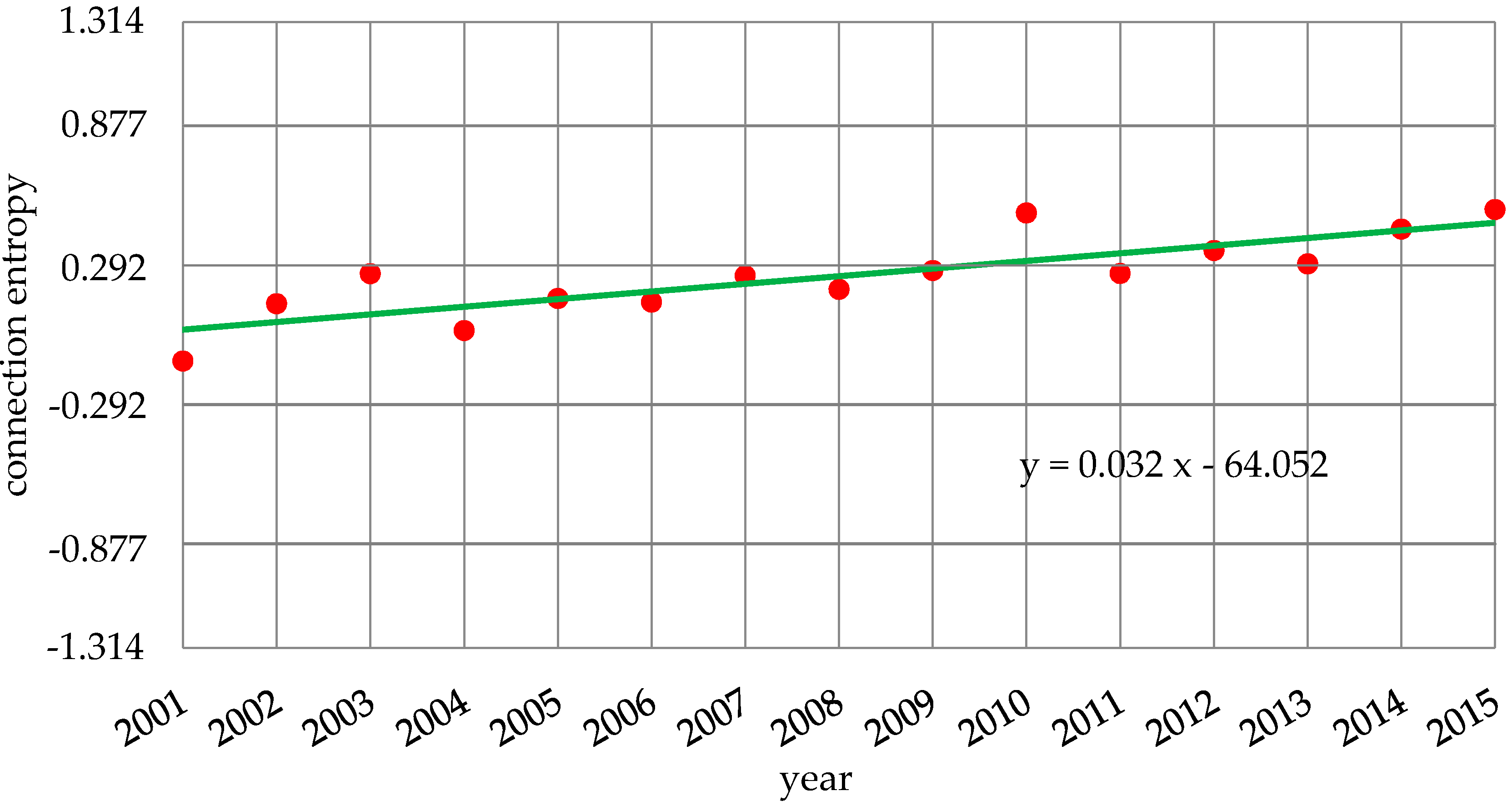
The value of the discrepancy entropy coefficients in Equation (16) can be measured with the application of the mean method [1]: , and . Moreover, the value of the contrary entropy coefficients, both J1 and J2, become equal to −1. Thus, the value of the synthesis of connection entropy of water resources vulnerability in Anhui Province is measured using Equation (16) and the findings are shown in Table 7. The curve for the synthesis of connection entropy of water resources vulnerability in Anhui Province is presented in Figure 2.
5.5. Synthesis of the Level of Water Resources Vulnerability in Anhui Province
5.6. Analysis of Results
The synthesis of the level of water resources vulnerability in Anhui Province appeared to be moderate in 2001–2009, and 2011, and slight in 2010, and 2012–2015 (Table 7). As evident from Figure 2, the following can be observed: the vulnerability level fluctuated and exhibited an apparent improving trend from 2001 to 2015.
The analysis of vulnerability of typical years is as follows: (1) the synthesis of the level of water resources vulnerability in 2003 was highest during 2001–2005 period as it was a wet year. The average annual rainfall was 1460.9 mm, which was 24.4% higher than the multi-year average. Water resources availability was 108.301 billion m3, which was 51.3% higher than the multi-year average. Thus, the vulnerability index water utilization rate was low, and the per unit area available amount of water resources was high. Good economic benefits are expected because of effective flood control and drought relief measures. (2) The synthesis of the level of water resources vulnerability in 2004 was the lowest during the 2002–2006 period as it was a low flow period. The average annual rainfall was 998.0 mm, 14.9% less than the multi-year average, and water resources availability was 50.065 billion m3, being 30.1% less than the multi-year average. Thus, the value of the vulnerability index water utilization rate was high, and that of the per unit area available amount of water resources was low, together with the per unit GDP of water consumption being high. (3) The synthesis of the level of water resources vulnerability in 2010 was the highest during the 2008–2012 period as it was a partially wet period. The average annual rainfall was 1308.90 mm, being 11.6% more than the multi-year average, and water resources availability was 93.905 billion m3, being 31.1% more than the multi-year average. Thus, the vulnerability index water utilization rate appears to be low, and the per unit area available amount of water resources is high, in addition to the reasonable economic benefits of flood control and fight drought.
6. Conclusions and Suggestions
From the finding presented in this paper, the following conclusions may be put forth:
- (1)
- This study considered the mechanism of water resources vulnerability in a changing environment, focusing on the analysis of four key states of a water system: sensitive state, damaged state, recovery state, and equilibrium state. The state of a water system generally changes from damaged to recovery via natural factors, followed by the transition from a state of recovery to one of equilibrium primarily because of artificial factors. The former is defined as natural resilience and the latter as artificial adaptation. This mechanism results offer much-needed insights into water resources vulnerability in a changing environment, but the mechanism of transformation process between four states is the focus of future research.
- (2)
- This paper proposed an analysis method to system uncertainty on the basis of connection entropy, extending the Zhao’s [1] original concept. In addition, our analysis of water resources vulnerability in Anhui Province, China showed that the vulnerability level fluctuated, as well as exhibiting apparent improvement trends over a 15-year period. The synthesize grade of water resources vulnerability in Anhui Province appeared to be moderate in 2001–2009, and 2011, and a slight in 2010, and 2012–2015.
- (3)
- The vulnerability level exhibited an apparent improving trend from 2001 to 2015, but still needs to be improved. There is a need to improve the perceptions of the vulnerability index, such as water utilization rate, per capita sewage discharge, surface water environment quality, per unit GDP of water consumption, and the economic benefits of flood control and fight drought.
Based on the results, we suggest the following improvements for water resources vulnerability in Anhui Province: on the one hand, there is an abated water resources sensitivity, whereby an increase in the reuse rate of industrial water can reduce water resources utilization. Moreover, sewage discharge can be reduced by the promotion of water saving policy and knowledge, encouraging water savings, and creating a greater awareness of (as well as building) a water-saving society. On the other hand, there is a need to improve natural resilience and artificial adaptation. Both can be achieved by developing sewage treatment to improve water environment quality, reduce high water consumption, eradicate backward industries, and promote new technology. Such actions will reduce the per unit GDP of water consumption and losses caused by floods and droughts, and improve the economic benefits of flood control and fight drought. Thus, for the purpose of ensuring sustainable development of economic, social and water resources in region, there is a need to improve the level of water resources vulnerability in the Anhui Province.
Acknowledgments
The authors would like to thank the support of the National Key Research and Development Program of China under Grant No. 2016YFC0401303 and No. 2016YFC0401305, the National Natural Science Foundation of China (Grant No. 51579059, No. 51509158, No. 51709071 and No. 51309004).
Author Contributions
Z.P. was responsible for the data analysis and code programming; Z.P. wrote the paper; R.Z. contributed the data; J.J. constructed the research framework and designed the study; C.L. and S.N. reviewed and edited the manuscript. All of the authors have read and approved the final manuscript.
Conflicts of Interest
The authors declare no conflict of interest.
References
- Zhao, K.Q. Set Pair Analysis and Preliminary Application; China Science Technology Press: Hangzhou, China, 2000. [Google Scholar]
- Turner, B.L., II; Kasperson, R.E.; Matson, P.A.; McCarthy, J.J.; Corell, R.W.; Christensen, L.; Eckley, N.; Kasperson, J.X.; Luers, A.; Martello, M.L.; et al. A framework for vulnerability analysis in sustainability science. Proc. Natl. Acad. Sci. USA 2003, 100, 8074–8079. [Google Scholar] [CrossRef] [PubMed]
- Füssel, H.M. Vulnerability: A generally applicable conceptual framework for climate change research. Glob. Environ. Chang. 2007, 17, 155–167. [Google Scholar] [CrossRef]
- Padowski, J.C.; Gorelick, S.M. Global analysis of urban surface water supply vulnerability. Environ. Res. Lett. 2014, 9, 104004. [Google Scholar] [CrossRef]
- Allouchea, N.; Maananb, M.; Gontaraa, M.; Rollob, N.; Jmala, I.; Bouria, S. A global risk approach to assessing groundwater vulnerability. Environ. Model. Softw. 2017, 88, 168–182. [Google Scholar] [CrossRef]
- Khakhar, M.; Ruparelia, J.P.; Vyas, A. Assessing groundwater vulnerability using GIS-based DRASTIC model for Ahmedabad district, India. Environ. Earth Sci. 2017, 76, 440. [Google Scholar] [CrossRef]
- Rushforth, R.R.; Ruddell, B.L. The vulnerability and resilience of a city’s water footprint: The case of Flagstaff, Arizona, USA. Water Resour. Res. 2016, 52, 2698–2714. [Google Scholar] [CrossRef]
- Martinez, S.; Kralisch, S.; Escolero, O.; Perevochtchikova, M. Vulnerability of Mexico City’s water supply sources in the context of climate change. J. Water Clim. Chang. 2015, 6, 518–533. [Google Scholar] [CrossRef]
- Padowski, J.C.; Jawitz, J.W. Water availability and vulnerability of 225 large cities in the United States. Water Resour. Res. 2012, 48. [Google Scholar] [CrossRef]
- Sullivan, C.A. Quantifying water vulnerability: A multi-dimensional approach. Stoch. Environ. Res. Risk Assess. 2011, 25, 627–640. [Google Scholar] [CrossRef]
- McCarthy, J.J.; Canziani, O.F.; Leary, N.A.; Dokken, D.J.; White, K.S. Climate Change 2001: Impacts, Adaptation, and Vulnerability. Contribution of Working Group II to the Third Assessment Report of the Intergovernmental Panel on Climate Change; Cambridge University Press: Cambridge, UK, 2001. [Google Scholar]
- Safi, A.S.; Smith, W.J.; Liu, Z. Vulnerability to climate change and the desire for mitigation. J. Environ. Stud. Sci. 2016, 6, 503–514. [Google Scholar] [CrossRef]
- Liersch, S.; Cools, J.; Kone, B.; Koch, H.; Diallo, M.; Reinhardt, J.; Fournet, S.; Aich, V.; Hattermann, F.F. Vulnerability of rice production in the Inner Niger Delta to water resources management under climate variability and change. Environ. Sci. Policy 2013, 34, 18–33. [Google Scholar] [CrossRef]
- Yang, X.H.; Sun, B.Y.; Zhang, J.; Li, M.S.; He, J.; Wei, Y.M.; Li, Y.Q. Hierarchy evaluation of water resources vulnerability under climate change in Beijing, China. Nat. Hazards 2016, 84, 63–76. [Google Scholar] [CrossRef]
- Gain, A.K.; Giupponi, C.; Renaud, F.G. Climate Change Adaptation and Vulnerability Assessment of Water Resources Systems in Developing Countries: A Generalized Framework and a Feasibility Study in Bangladesh. Water 2012, 4, 345–366. [Google Scholar] [CrossRef] [Green Version]
- Ionescu, C.; Klein, R.J.T.; Hinkel, J.; Kumar, K.S.K.; Klein, R. Towards a Formal Framework of Vulnerability to Climate Change. Environ. Model. Assess. 2009, 14, 1–16. [Google Scholar] [CrossRef]
- Al-Saidi, M.; Birnbaum, D.; Buriti, R.; Diek, E.; Hasselbring, C.; Jimenez, A.; Woinowski, D. Water Resources Vulnerability Assessment of MENA Countries Considering Energy and Virtual Water. Procedia Eng. 2016, 145, 900–907. [Google Scholar] [CrossRef]
- Shabbir, R.; Ahmad, S.S. Water resource vulnerability assessment in Rawalpindi and Islamabad, Pakistan using Analytic Hierarchy Process (AHP). J. King Saud Univ. Sci. 2016, 28, 293–299. [Google Scholar] [CrossRef]
- Pan, Z.; Jin, J.; Wu, K.; Res, K.D. Earch on the Indexes and Decision Method of Regional Water Environmental System Vulnerability. Resour. Environ. Yangtze Basin 2014, 23, 518–525. [Google Scholar] [CrossRef]
- Field, C.B.; Barros, V.R.; Dokken, D.J.; Mavh, K.J.; Mastrabdrea, M.D.; Bilir, T.E.; Chatterjee, M.; Ebi, K.L.; Estrada, Y.O.; Genova, R.C.; et al. (Eds.) Climate Change 2014: Impacts, Adaptation, and Vulnerability. Summaries, Frequently Asked Questions, and Cross-Chapter Boxes. A Contribution of Working Group II to the Fifth Assessment Report of the Intergovernmental Panel on Climate Change; World Meteorological Organization: Geneva, Switzerland, 2014. [Google Scholar]
- Hassan, R.; Scholes, R.; Ash, N. (Eds.) Appendix D: Glossary. In Ecosystems and Human Well-being: Current States and Trends; Island Press: Washington, DC, USA, 2005; Volume 1, pp. 893–900. [Google Scholar]
- Hartley, R.V. Transmission of Information. Bell Syst. Tech. J. 1928, 7, 535–563. [Google Scholar] [CrossRef]
- Schrödinger, E. What Is Life? The Physical Aspects of Living Cell; Cambridge University Press: Cambridge, UK, 1944. [Google Scholar]
- Shannon, C.E. A mathematical theory of communication. Bell Syst. Tech. J. 1948, 27, 379–423. [Google Scholar] [CrossRef]
- De Luca, A.; Termini, S. A definition of a nonprobabilistic entropy in the setting of fuzzy sets. Inf. Control. 1972, 20, 301–312. [Google Scholar] [CrossRef]
- Zhao, K. Study on set pair analysis and entropy. J. Zhejiang Univ. 1992, 6, 65–72. [Google Scholar]
- Su, M.R.; Yang, Z.F.; Chen, B. Set pair analysis for urban ecosystem health assessment. Commun. Nonlinear Sci. Numer. Simul. 2009, 14, 1773–1780. [Google Scholar] [CrossRef]
- Wang, W.; Jin, J.; Ding, J.; Li, Y. A new approach to water resources system assessment―Set pair analysis method. Sci. China Ser. E Technol. Sci. 2009, 52, 3017–3023. [Google Scholar] [CrossRef]
- Kumar, K.; Garg, H. TOPSIS method based on the connection number of set pair analysis under interval-valued intuitionistic fuzzy set environment. Comput. Appl. Math. 2016, 1–11. [Google Scholar] [CrossRef]
- Pan, Z.; Wang, Y.; Jin, J.; Liu, X. Set pair analysis method for coordination evaluation in water resources utilizing conflict. Phys. Chem. Earth 2017. [Google Scholar] [CrossRef]
- Pan, Z.; Wu, C.; Jin, J. Set Pair Analysis Methods for Water Resource System Evaluation and Prediction; Science Press: Beijing, China, 2016. [Google Scholar]
- Jin, J.; Wei, Y. Generalized Intelligent Evaluation Method for Complex System and Its Application; Science Press: Beijing, China, 2008. [Google Scholar]
Figure 1.
Mechanism diagram of water resources vulnerability in changing environment.
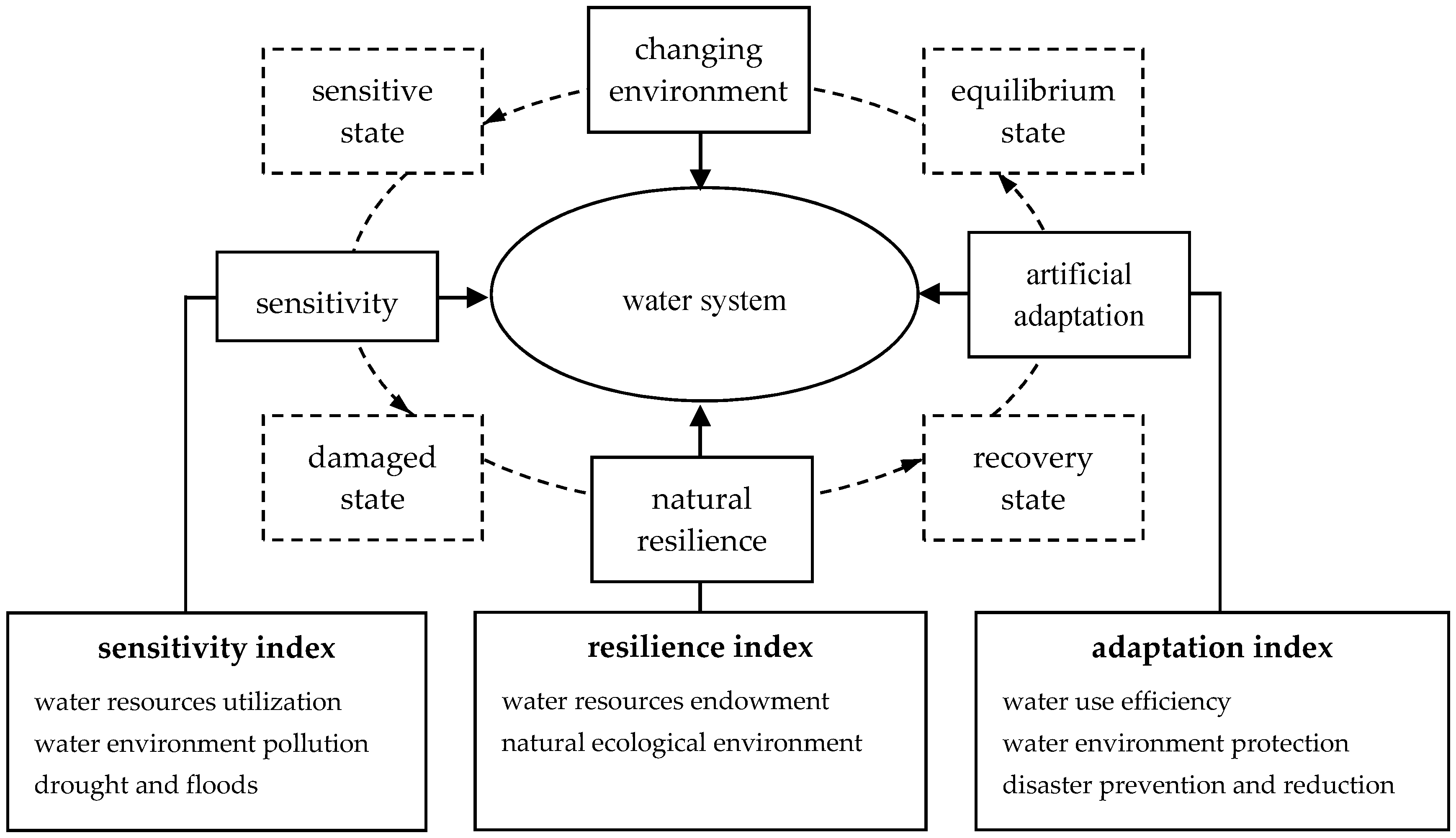
Figure 2.
Synthesize connection entropy trend line of water resources vulnerability in Anhui Province.
Figure 2.
Synthesize connection entropy trend line of water resources vulnerability in Anhui Province.

Table 1.
Sensitive index of water resources.
| Sensitive Factor | Sensitive Index | |
|---|---|---|
| Water resources utilization | x1 | Water utilization rate (%) |
| Water environment pollution | x2 | Emission intensity of industrial wastewater (t/104ұ) |
| x3 | Per capita sewage discharge (t/person) | |
| Drought and floods | x4 | Proportion of economic losses of water disasters to GDP (%) |
Table 2.
Resilient index of water resources.
| Resilient Factor | Resilient Index | |
|---|---|---|
| Water resources endowment | x5 | Per unit area available amount of water resources (104·m3/km2) |
| Water environmental quality | x6 | Surface water environment quality (%) |
| Eco-environmental quality | x7 | Forest cover (%) |
Table 3.
Adaptive index of water resources.
| Adaptive Factor | Adaptive Index | |
|---|---|---|
| Water use efficiency | x8 | Per unit GDP of water consumption (m3/104ұ) |
| Water environment protection | x9 | Compliance rate of industrial wastewater (%) |
| x10 | Treatment rate of urban sewage (%) | |
| Disaster prevention and reduction | x11 | Economic benefits of flood control and fighting drought (108ұ) |
Table 4.
Standard interval of the vulnerability index in Anhui Province.
| Index | Standard Interval | |||||
|---|---|---|---|---|---|---|
| Low (I) | Slight (II) | Moderate (III) | High (IV) | Extreme (V) | ||
| Sensitive | x1 (%) | 0–10 | 10–25 | 25–40 | 40–60 | 60–100 |
| x2 (t/104Ұ) | 0–10 | 10–25 | 25–40 | 40–55 | 55–100 | |
| x3 (t/person) | 0–5 | 5–10 | 10–40 | 40–60 | 60–100 | |
| x4 (%) | 0–1.0 | 1.0–2.5 | 2.5–4.0 | 4.0–4.5 | 4.5–5.5 | |
| Natural resilience | x5 (104·m3/km2) | 75–100 | 55–75 | 35–55 | 15–35 | 5–15 |
| x6 (%) | 90–100 | 80–90 | 70–80 | 50–70 | 0–50 | |
| x7 (%) | 30–50 | 20–30 | 15–20 | 10–15 | 5–10 | |
| Artificial adaptation | x8 (m3/104Ұ) | 5–24 | 24–140 | 140–610 | 610–1060 | 1060–1600 |
| x9 (%) | 97.5–100 | 92.5–97.5 | 85–92.5 | 80–85 | 15–80 | |
| x10 (%) | 80–100 | 60–80 | 40–60 | 20–40 | 0–20 | |
| x11 (108Ұ) | 400–600 | 200–400 | 100–200 | 60–100 | 0–60 | |
Table 5.
Index data of the vulnerability index in Anhui Province in 2001–2015.
| Year | x1 | x2 | x3 | x4 | x5 | x6 | x7 | x8 | x9 | x10 | x11 |
|---|---|---|---|---|---|---|---|---|---|---|---|
| 2001 | 45.22 | 17.79 | 11.47 | 3.13 | 34.00 | 41.00 | 27.95 | 603.56 | 95.24 | 7.84 | 128.00 |
| 2002 | 25.36 | 16.90 | 12.27 | 1.48 | 59.13 | 51.08 | 27.95 | 588.48 | 95.74 | 15.80 | 91.80 |
| 2003 | 16.83 | 14.88 | 12.13 | 5.72 | 77.65 | 48.69 | 27.95 | 458.79 | 95.88 | 20.14 | 440.67 |
| 2004 | 41.89 | 13.31 | 13.04 | 0.74 | 35.90 | 41.70 | 30.30 | 435.80 | 96.91 | 25.69 | 70.00 |
| 2005 | 28.92 | 10.89 | 14.29 | 3.49 | 51.57 | 44.30 | 26.06 | 386.10 | 97.36 | 31.28 | 209.00 |
| 2006 | 41.67 | 11.40 | 14.61 | 1.00 | 41.62 | 64.60 | 26.06 | 393.80 | 97.12 | 32.90 | 145.30 |
| 2007 | 32.60 | 9.99 | 15.24 | 1.98 | 51.80 | 64.70 | 26.06 | 305.90 | 94.77 | 37.64 | 420.50 |
| 2008 | 38.09 | 8.29 | 15.08 | 2.41 | 50.13 | 69.30 | 26.06 | 288.80 | 96.17 | 52.08 | 100.00 |
| 2009 | 39.81 | 7.30 | 15.64 | 1.44 | 52.56 | 72.10 | 26.06 | 290.04 | 96.21 | 72.81 | 86.00 |
| 2010 | 31.15 | 5.74 | 16.66 | 0.92 | 67.33 | 77.70 | 27.53 | 238.50 | 97.67 | 77.75 | 260.00 |
| 2011 | 48.94 | 4.62 | 25.07 | 0.61 | 43.17 | 65.50 | 27.53 | 195.00 | 97.47 | 79.04 | 145.00 |
| 2012 | 41.16 | 3.90 | 27.09 | 0.28 | 50.26 | 70.60 | 27.53 | 167.60 | 98.38 | 86.39 | 154.80 |
| 2013 | 50.55 | 3.73 | 28.16 | 0.80 | 41.99 | 72.40 | 27.53 | 155.50 | 98.51 | 88.44 | 187.10 |
| 2014 | 34.95 | 3.34 | 29.20 | 0.14 | 55.81 | 77.90 | 28.65 | 131.00 | 98.69 | 90.19 | 103.11 |
| 2015 | 31.58 | 3.25 | 30.07 | 0.34 | 65.54 | 81.80 | 28.65 | 131.20 | 98.70 | 91.80 | 136.89 |
Sources: Statistics Bureau of Anhui Province, 2002–2016, and Water Resources Bulletin of Anhui Province, 2001–2015.
Table 6.
Connection entropy of vulnerability index in 2015.
| Index | Connection Entropy | wj |
|---|---|---|
| x1 | S15,1 = 0.0000 + 0.0000 + 0.3083I1 + 0.5844I2 + 0.2363I3 + 0.0000J1 + 0.0000J2 | 0.120 |
| x2 | S15,2 = 0.3772 + 0.5844 + 0.1717I1 + 0.0000I2 + 0.0000I3 + 0.0000J1 + 0.0000J2 | 0.100 |
| x3 | S15,3 = 0.0000 + 0.0000 + 0.1754I1 + 0.5844I2 + 0.3732I3 + 0.0000J1 + 0.0000J2 | 0.100 |
| x4 | S15,4 = 0.3691 + 0.5844 + 0.1791I1 + 0.0000I2 + 0.0000I3 + 0.0000J1 + 0.0000J2 | 0.080 |
| x5 | S15,5 = 0.0000 + 0.2879 + 0.5844I1 + 0.2562I2 + 0.0000I3 + 0.0000J1 + 0.0000J2 | 0.150 |
| x6 | S15,6 = 0.0000 + 0.0929 + 0.5844I1 + 0.4676I2 + 0.0000I3 + 0.0000J1 + 0.0000J2 | 0.090 |
| x7 | S15,7 = 0.0000 + 0.4964 + 0.5844I1 + 0.0692I2 + 0.0000I3 + 0.0000J1 + 0.0000J2 | 0.060 |
| x8 | S15,8 = 0.0000 + 0.0385 + 0.5844I1 + 0.5346I2 + 0.0000I3 + 0.0000J1 + 0.0000J2 | 0.090 |
| x9 | S15,9 = 0.2603 + 0.5844 + 0.2838I1 + 0.0000I2 + 0.0000I3 + 0.0000J1 + 0.0000J2 | 0.075 |
| x10 | S15,10 = 0.3254 + 0.5844 + 0.2199I1 + 0.0000I2 + 0.0000I3 + 0.0000J1 + 0.0000J2 | 0.075 |
| x11 | S15,11 = 0.0000 + 0.0000 + 0.1966I1 + 0.5844I2 + 0.3502I3 + 0.0000J1 + 0.0000J2 | 0.060 |
| ∑ | S15 = 0.1112 + 0.2776 + 0.3635I1 + 0.2964I2 + 0.0867I3 + 0.0000J1 + 0.0000J2 |
Table 7.
Synthesize connection entropy of water resources vulnerability in Anhui Province.
| Year | Synthesize Connection Entropy | Value | Grade |
|---|---|---|---|
| 2001 | S1 = 0.0000 + 0.0757 + 0.2358I1 + 0.3786I2 + 0.3047I3 + 0.1166J1 + 0.0336J2 | −0.109 | III |
| 2002 | S2 = 0.0000 + 0.1302 + 0.3956I1 + 0.3372I2 + 0.1765I3 + 0.0996J1 + 0.0082J2 | 0.132 | III |
| 2003 | S3 = 0.0144 + 0.2517 + 0.3810I1 + 0.2092I2 + 0.1793I3 + 0.1082J1 + 0.0012J2 | 0.258 | III |
| 2004 | S4 = 0.0113 + 0.1641 + 0.2431I1 + 0.2964I2 + 0.3117I3 + 0.1139J1 + 0.0077J2 | 0.019 | III |
| 2005 | S5 = 0.0000 + 0.1185 + 0.3924I1 + 0.3888I2 + 0.1694I3 + 0.0702J1 + 0.0052J2 | 0.154 | III |
| 2006 | S6 = 0.0002 + 0.1593 + 0.2956I1 + 0.3815I2 + 0.2750I3 + 0.0320J1 + 0.0000J2 | 0.138 | III |
| 2007 | S7 = 0.0032 + 0.1468 + 0.3988I1 + 0.4082I2 + 0.1678I3 + 0.0170J1 + 0.0000J2 | 0.249 | III |
| 2008 | S8 = 0.0088 + 0.1120 + 0.3518I1 + 0.4649I2 + 0.2066I3 + 0.0016J1 + 0.0000J2 | 0.192 | III |
| 2009 | S9 = 0.0142 + 0.1683 + 0.3773I1 + 0.3927I2 + 0.1788I3 + 0.0112J1 + 0.0000J2 | 0.271 | III |
| 2010 | S10 = 0.0287 + 0.2735 + 0.4791I1 + 0.3001I2 + 0.0585I3 + 0.0000J1 + 0.0000J2 | 0.513 | II |
| 2011 | S11 = 0.0462 + 0.2157 + 0.2949I1 + 0.3195I2 + 0.2225I3 + 0.0395J1 + 0.0000J2 | 0.259 | III |
| 2012 | S12 = 0.0928 + 0.2184 + 0.2810I1 + 0.3596I2 + 0.1864I3 + 0.0035J1 + 0.0000J2 | 0.355 | II |
| 2013 | S13 = 0.0763 + 0.2184 + 0.2807I1 + 0.3248I2 + 0.2020I3 + 0.0346J1 + 0.0000J2 | 0.299 | II |
| 2014 | S14 = 0.1166 + 0.2293 + 0.3222I1 + 0.3520I2 + 0.1236I3 + 0.0000J1 + 0.0000J2 | 0.445 | II |
| 2015 | S15 = 0.1112 + 0.2776 + 0.3635I1 + 0.2964I2 + 0.0867I3 + 0.0000J1 + 0.0000J2 | 0.527 | II |
© 2017 by the authors. Licensee MDPI, Basel, Switzerland. This article is an open access article distributed under the terms and conditions of the Creative Commons Attribution (CC BY) license (http://creativecommons.org/licenses/by/4.0/).
Share and Cite
MDPI and ACS Style
Pan, Z.; Jin, J.; Li, C.; Ning, S.; Zhou, R. A Connection Entropy Approach to Water Resources Vulnerability Analysis in a Changing Environment. Entropy 2017, 19, 591. https://doi.org/10.3390/e19110591
AMA Style
Pan Z, Jin J, Li C, Ning S, Zhou R. A Connection Entropy Approach to Water Resources Vulnerability Analysis in a Changing Environment. Entropy. 2017; 19(11):591. https://doi.org/10.3390/e19110591
Chicago/Turabian StylePan, Zhengwei, Juliang Jin, Chunhui Li, Shaowei Ning, and Rongxing Zhou. 2017. "A Connection Entropy Approach to Water Resources Vulnerability Analysis in a Changing Environment" Entropy 19, no. 11: 591. https://doi.org/10.3390/e19110591
Note that from the first issue of 2016, this journal uses article numbers instead of page numbers. See further details here.