A Novel Derivation of the Time Evolution of the Entropy for Macroscopic Systems in Thermal Non-Equilibrium


Department of Mechanical & Aerospace Engineering, University of Roma Sapienza, 00184 Roma, Italy
*
Author to whom correspondence should be addressed.
Entropy 2017, 19(11), 594; https://doi.org/10.3390/e19110594
Submission received: 30 June 2017
/
Revised: 20 October 2017
/
Accepted: 4 November 2017
/
Published: 7 November 2017
(This article belongs to the Special Issue Entropy, Time and Evolution)
Abstract
:The paper discusses how the two thermodynamic properties, energy (U) and exergy (E), can be used to solve the problem of quantifying the entropy of non-equilibrium systems. Both energy and exergy are a priori concepts, and their formal dependence on thermodynamic state variables at equilibrium is known. Exploiting the results of a previous study, we first calculate the non-equilibrium exergy En-eq can be calculated for an arbitrary temperature distributions across a macroscopic body with an accuracy that depends only on the available information about the initial distribution: the analytical results confirm that En-eq exponentially relaxes to its equilibrium value. Using the Gyftopoulos-Beretta formalism, a non-equilibrium entropy Sn-eq(x,t) is then derived from En-eq(x,t) and U(x,t). It is finally shown that the non-equilibrium entropy generation between two states is always larger than its equilibrium (herein referred to as “classical”) counterpart. We conclude that every iso-energetic non-equilibrium state corresponds to an infinite set of non-equivalent states that can be ranked in terms of increasing entropy. Therefore, each point of the Gibbs plane corresponds therefore to a set of possible initial distributions: the non-equilibrium entropy is a multi-valued function that depends on the initial mass and energy distribution within the body. Though the concept cannot be directly extended to microscopic systems, it is argued that the present formulation is compatible with a possible reinterpretation of the existing non-equilibrium formulations, namely those of Tsallis and Grmela, and answers at least in part one of the objections set forth by Lieb and Yngvason. A systematic application of this paradigm is very convenient from a theoretical point of view and may be beneficial for meaningful future applications in the fields of nano-engineering and biological sciences.
1. Introduction
1.1. Definition of Scope
This paper presents a derivation of the entropy evolution in macroscopic systems initially out of equilibrium. The derivation begins by showing that for any given macroscopic system it is possible, under certain very general assumptions, to calculate a “non-equilibrium exergy” by analytically solving the diffusion and the thermodynamic equations. Once it is accepted that exergy—under the above mentioned assumptions—is well-defined and measurable for systems not extremely remote from their equilibrium, as long as the energy of a system is known (it is given by the initial T distribution), a non-equilibrium entropy can be derived which reduces in the limit to the standard definition when the initial state of the system is an equilibrium one.
The procedure is based only on physical and classical first-order thermodynamic reasoning (heat and mass diffusion laws), and no new axiom is invoked except for the local equilibrium assumption. It is presented here for a continuum, but an extension to finite ensembles of interacting homogeneous particles is possible. Even if the procedure implies the local equilibrium assumption, and its degree of accuracy is perfectly satisfactory as long as the relevant scales of the problem are such that the continuum hypothesis holds. The method falls within the frame of Classical Irreversible Thermodynamics (CIT), and the conclusions we reach in this study are placed in a more general context by comparing their qualitative and quantitative aspects with microscopic theories like Tsallis’ entropy [1] and with the multi-scale hypothesis of Grmela et al. [2]. Furthermore, our results overcome the problem raised by Lieb and Yngvason [3] about the non-physicality of a unique and monotonic entropy function in the non-equilibrium realm.
The possibility of rigorously extending the definition of entropy to encompass non-equilibrium states is of great interest in all scientific fields dealing with systems that, from the very small to the very large, exist only in non-equilibrium conditions. The analysis of chemical processes in cells [4,5], atmospheric cycles [6] and complex living and non-living systems [2,7,8,9,10] would be simpler if a generally valid description of the evolution of fundamental thermodynamic quantities in non-equilibrium regions were at hand. From a microscopic point of view, the relaxation of non-equilibrium physical systems towards equilibrium has been derived in [11] using the principle of steepest entropy ascent. Here our point of view is different: as we will explain, it is based on macroscopic phenomenological assumptions and, in the limit of these assumptions, it is exact and rigorous. For these reasons, we believe that our approach is amenable to a lot more of applications than most of other non-equilibrium formulations.
It was shown [12] that the exergy destruction can, under a reasonable set of conditions, be taken as the Lagrangian of the Stokes-Navier equations (see also [13] for a detailed discussion). A derivation of the non-equilibrium exergy was published by the present authors [14] and the calculations were applied to one-, two-, and three-dimensional domains in thermal non-equilibrium. Once the energy and the exergy of an evolving system are known in space and time, the entropy of the system can be computed from the definition of the exergy (E = U − T0S):
Equation (1) is in fact the non-equilibrium extension proposed by Haftopoulos and Gyftopoulos [15,16,17], Gyftopoulos and Beretta [18] and Beretta [19] (it must be mentioned that an opposite point of view exists (Gaggioli [20,21,22]), that postulates the existence of a quantity called “non-equilibrium entropy” and derives Equation (7) as a corollary. In response to a Reviewer’s remark, we are well aware that Equation (1) is in fact derived in [15,16,17,18], and as such it would be correct to state it as a theorem: our considering it here an assumption is in reality a weaker position). In the remainder of this paper, all applications refer, for simplicity, to solid bodies. The extension to systems consisting—in part or in toto—of variable density media (specifically, of gases) is immediate, and begins with the substitution of the enthalpy H in lieu of the internal energy U in Equation (1). The expression (1) does not require the introduction of a “non-equilibrium temperature”, since T0 is the uniform and constant value of the temperature of the reference thermal bath (the “environment”). It will be shown below that, since there may exist several iso-energetic states with different internal energy distributions, and upon relaxation from an initial non-equilibrium state to a final one in equilibrium all or part of the energy is either redistributed or exchanged with the remaining universe, while the exergy history depends precisely on the degree of internal inhomogeneity (i.e., of departure from equilibrium), the entropy defined by Equation (1) is multi-valued. This means that two twin systems prepared in such a way as to be iso-energetic at time t0 but having—for instance—different internal temperature distributions T1(x, t0) and T2(x, t0), have different initial entropies and shall evolve towards equilibrium along two uncorrelated paths, with possibly very different entropy generation rates even under the same boundary conditions for t > t0. This feature may appear obvious and even intuitive, but our method provides a quantification of this effect.
1.2. On the Existence of a Non-Equilibrium Entropy Function
Classical Thermodynamics deals with systems “in equilibrium”, where the system (solid or fluid, simple or composite, continuous or discrete) is in a certain physical state described by a set of state variables whose variables are independent of time: no internal changes, no mass- or energy exchange with other systems, are allowed (it is possible to include under this definition the so-called ideal steady-state processes, if their inherent dynamics are “lumped” by assuming that the mass- and energy flows through their boundaries remain unchanged in time. Such—strongly idealized—processes may display a constant value of the system’s entropy). “Time” is not a variable in equilibrium thermodynamics, but it is experimental evidence has proven that, both in nature and in real engineering applications, an equilibrium system constitutes a useful approximation that leads to first-order estimates of the energy exchanges between the system and the surroundings, while neglecting most or even all of the internal dynamics of the system itself. Even in the most accurate, and in some tutorial cases, exact descriptions of such systems, any change in the imposed constraints, like the removal of a rigid or an adiabatic partition, would generate internal mass- and/or energy exchanges that can be described only in terms of time-dependent processes. To adapt equilibrium thermodynamics into the realm of real processes, the concepts of quasi-equilibrium and quasi-reversible process were introduced, by assuming that a system evolves in time from one state to the other through an infinite series of very small steps taking place along an “equilibrium path”. This is a very successful approximation that led to the construction of which is a vast body of theoretical knowledge, and is at the basis of innumerable successful applications in all scientific fields.
In engineering applications, the discrepancy between the “ideal, equilibrium” behavior and that of the real system is handled by introducing numerical corrections into the model by means of properly defined coefficients that go under the name of “efficiencies”: the effects of the internal derangement from homogeneity result in a final state that is different from the one predicted by the “quasi-equilibrium” assumption, which suggests that the real path of the transformation was in fact different from the postulated one. In such cases it is necessary to conclude that, since energy is on the whole conserved, the “lost work” is converted into “irreversible entropy generation” causing a shift of a portion of the “ideal” work (or heat) towards the molecular or atomic scales of the participating media and increasing the temperature of the final state.
The non-equilibrium thermodynamic systems considered in this study are spatially and temporally non-uniform, but their non-uniformity is sufficiently smooth to allow for the definition of suitable time and space derivatives of non-equilibrium state variables. To account for spatial non-uniformity, extensive non-equilibrium state variables are defined as spatial densities of the corresponding extensive equilibrium state variables. If the system is sufficiently close to thermodynamic equilibrium, intensive non-equilibrium state variables like temperature and pressure take on values close to the equilibrium ones; further away from equilibrium, the problem becomes more complex, and one of the possibilities is to consider their gradients (spatial and temporal) as additional independent variables of the problem, and suitable boundary and initial conditions must be assigned. This is the Extended Irreversible Thermodynamics approach [23,24,25]. A quite different paradigm is proposed by the so-called Quantum Thermodynamics Theory (QT in the following) [26] and by its more recent development, Steepest-Entropy-Ascent Quantum Thermodynamics (SEAQT) [11]: in the former, the evolution of the system is described by a non-linear evolution equation, sum of the Hamiltonian term and a nonlinear, entropy-generating term. In SEAQT [11], an arbitrary isolated system in non-equilibrium is studied using the principle of steepest entropy ascent reformulated in a variational form. Their model makes no use of the local equilibrium assumption, and expresses the conjugate fluxes and forces by means of the novel concepts of hypo-equilibrium state and non-equilibrium intensive properties, which describe the non-mutual equilibrium status between subspaces of the thermodynamic state space. SEAQT rederives the Onsager relations and can describe the behavior of the system in far-from-equilibrium regions. In the present study, we do not use the Steepest Entropy Ascent assumption but introduce the “local equilibrium assumption”, which considers each very small spatial subdomain of the system as being homogeneous, well-mixed, and without a discernible spatial structure. As a consequence, the local entropy density is the same function of the other local intensive variables as it is in equilibrium. This amounts to assuming spatial and temporal continuity and differentiability of all locally defined intensive variables such as temperature and internal energy density, and results in the possibility of computing the global entropy of the system by integrating its local counterpart over the domain of interest. This approach obviously may fail at the smallest scales, where local derivatives may not exist or be discontinuous, but deals rather well with the large majority of observable phenomena at the so-called macro- and mesoscales, as long as the characteristic time defined as the ratio of the square of the domain dimension to the thermal diffusivity, τ = δx2/α, is larger than the molecular timescales. The practical usefulness of this approach is enormous. It suffices here to mention that all the thermo-fluid codes based on finite-volume or finite-element discretizations are in fact instantiations of the local equilibrium method.
When studying a non-equilibrium system, the first question one should answer is: are we interested in its global entropy and its time evolution or also in the behavior of the local entropy density? Since the former is derived by integrating the latter, it would seem that our goal is to calculate the local entropy density. However, in real cases we apply standard transport equations and physical laws (e.g., Fourier or Cattaneo for heat diffusion, Fick’s law for mass diffusion, energy transport equations in fluids etc.) to calculate the local entropy density, and therefore the emphasis is shifted to the dynamics of the global entropy of the system. In logical terms, this is an initial value problem for the system as a whole, but the equations that rule the internal smoothing of the gradients are in general parabolic and therefore the “driving forces” that guide the system’s evolution towards equilibrium or towards a different non-equilibrium state are dictated by both the initial conditions of the system (e.g., the distribution of mass and energy at the time of the opening of the window of observation) and by the (possibly time-dependent) boundary conditions. In other words, the local subdomains exchange different energy fluxes in such a way as to smooth out the initial spatially inhomogeneous energy distribution, but these fluxes—and as a consequence S(x, t), which is assumed here to exist in the form of Equation (1)—depend at each instant of time on the prevailing boundary conditions on the system’s external frontier. It looks like we are dealing with a multi-valued function, which therefore is often considered to be of a completely different nature than its equilibrium counterpart. In [27] the concept of entropy is rigorously derived from the definition of pure weight processes (pure mechanical work) and from the assumption that in the neighborhood of any given state A of a system there exist states of non-equilibrium from which A can return to equilibrium by means of zero-work processes. Here the context is different: since it is generally accepted that exergy is a proper indicator of the degree of irreversibility in a process [28], it appears to be the proper function to use in the description of the evolution of a system in the non-equilibrium domain. Incidentally, this is in line with Gibbs’ original definition of available energy that clearly envisioned a “relaxation process” from a non-equilibrium state to an equilibrium one through which some energy could be made “available”. However, there is no general agreement on the existence of such a quantity, and the only systematic treatment of the concept of non-equilibrium exergy is a paper by the present authors [14]. The scope of this paper is to use the Gyftopoulos–Beretta formulation to derive a “time-dependent entropy function” from the exergy E(x,t) and internal energy U(x,t) of a system to show that entropy is - under the assumptions postulated herein - a quantity defined equally well for equilibrium and non-equilibrium macroscopic systems.
2. Energy and Exergy
2.1. Energy
Consider an arbitrary system P of mass M known to be in an initial non-equilibrium state P(t = 0) of non-equilibrium. If the relevant scales are sufficiently removed from the smallest ones (those identified by statistical mechanical behavior), and if the gradients of the relevant measurables remain bounded throughout the system, we can subdivide P(t = 0) into a finite number k of spatial domains δPj such that , with each domain small enough to be considered in local equilibrium within the timescales imposed by the evolution of P. Each one of these domains has a measurable energy (notice that in the following formula uj is the TOTAL energy of the mass let mj, and is measured in J. For simplicity we assume hereafter the specific heat to be constant. The reference state is assumed to be the “dead state” at p0, T0, V0, …):
and thus both the total and the specific energy of P at the time t = 0 are computable as well, i.e.,:
At any other instant τ = t0 + dt, consider now another finite number n, not necessarily equal to k, of spatial domains, each one still small enough to be considered in local equilibrium within the prevailing timescales between t0 and t = τ: the energy of the (closed) system is:
Since the time interval τ is arbitrary, the evolution of the energy of the system is:
where dU/dt denotes the “infinitesimal” (continuous or finite) variation in time of the system’s energy. If P is isolated, then U(t) = U(0) at any time, and the evolution shall consist of a pure redistribution of the energy among the small spatial subdomains in which P is divided. If P can exchange energy with the external world, then dU/dt is dictated by the prevailing boundary conditions.
2.2. Availability and Exergy
Gibbs [29] defined an available energy or availability A as a thermodynamic function representing the maximum work that can be extracted from a system that proceeds from an initial arbitrary state to its final equilibrium state. In Gibbs’ original formulation, no restraint is imposed on the initial state of the system, and the system is assumed to be isolated [22]. Under the assumptions posited here, each subdomain j of P has therefore a computable (or measurable) available energy. Since the final state of the system is assumed to be an equilibrium state, (which implies complete homogeneity for any j), the total availability of the initial state can be calculated as the integral in time of the sum of the individual availabilities of each of the individual sub-domains:
Notice that neither the Gibbs’ available energy nor the adiabatic availability of Gyftopoulos and Beretta are additive: each subdomain j possesses at each instant of time 0 < t < τ an available energy aJ that depends on the “energetic and entropic distance” of j from the final “internal” equilibrium state. This means that Equation (7) must be interpreted as an infinite sum (in time) of the corresponding “system pictures” taken at each instant of time. When the process is completed, the system is in internal equilibrium, though not necessarily at its dead state, at a time t. If we introduce the possibility that in the time interval [0, t] P(τ) interacts with an external reference environment, its exergy is classically defined as the maximum work that can be extracted from this exclusive interaction such that:
where the sum implies that the boundary interactions may result in some internal non-uniformity (gradient of some or all of the thermodynamic quantities throughout P). Since, at time τ, P is in equilibrium, the “classical” definition of the exergy is valid for the entire system, namely:
Extending the above reasoning to initial non-equilibrium states, let us now define the non-equilibrium exergy of P(t = 0):
It can be shown that the latter quantity is always larger than the equilibrium exergy (Equation (8)) and is equal to the available energy only in the very special case in which the final state of the isolated system is the so-called dead state, i.e., all of its thermodymanic properties are identical to those of the reference state. We therefore maintain that Equation (10) describes the evolution of non-equilibrium systems in a more general way than Equation (7).
Since exergy is additive, the terms ej in (8) can also be computed directly, considering the evolution of each j-th subdomain from its initial local state δPj(t = 0) to its final dead state δPj(t = tfin) = (p0, T0, c0, V0, …). To perform this calculation, a complete specification of the reference state and of the boundary conditions must be provided at every instant of time.
3. Entropy Evolution in a Solid in an Initial Non-Equilibrium State
Let us consider a given solid body of known mass (spanning a spatial domain one-, two-, or three dimensional) with an initial temperature distribution and assume that the internal temperature throughout the body evolves according to Fourier’s law. We shall refer in general to the mass distribution as “the solid”.
The Fourier model for the heat conduction equation in solids under convective boundary conditions is:
where T0 is the temperature of the environment, is the boundary of the solid, is the local outward normal to the boundary and α is a measure of the heat transfer by convection at the boundaries. Taking the temperature of the immediate surroundings T0 as reference, we can calculate the exergy of the solid as a function of time. In the second of Equation (11), α is different from zero, since the problem implies a thermal exchange on all or part of the boundary between the solid and the environment. The contribution to the total exergy from each particle of solid at location and time t is:
where cv,j is the specific heat of the material that may be dependent on the local temperature.
The instantaneous contribution to the non-equilibrium exergy at time t is calculated in [14] as
where V is the volume of the solid and C its heat capacity. The cumulative amount of exergy at time is given by the difference between the exergy at time 0, E(0), and the exergy at time t, E(t). The total non-equilibrium exergy is then found by taking the limit , i.e., by the difference .
The equilibrium exergy of the system is given by:
Recalling that Teq = , the difference between the total non-equilibrium exergy and the exergy Ecl corresponding to an equilibrium transformation can be written, in the case of an environment at constant temperature and considering, for simplicity, the case of constant heat capacity, as:
The quantity calculated by Equation (15) is always non-negative (this follows directly from Jensen’s inequality for concave functions), and this leads to the important conclusion that the non-equilibrium exergy E (Equation (13)) is always greater than (or at most equal to) the classical equilibrium exergy Ecl (Equation (15)).
If temperature gradients on the surface of the solid still exist for t → ∞, they will generate convective heat exchanges at large times. This may happen when the temperature on the boundary of the solid is not uniform, a common engineering example being the convective fin, whose root is in thermal contact with a large mass at constant temperature while the fin surface and the tip exchange heat by convection with the environment at a fixed temperature: in this case the exergy of the system “fin” will assume a constant value—different from zero—for t → ∞. In this and all similar cases it is more convenient to analyze the evolution of the irreversible exergy destruction inside of the solid, as explained in [14].
Since the energy of the system is known at each instant of time, i.e.,:
Equation (1) provides the sought after expression for the instantaneous entropy, namely:
4. A Non-Conservative Evolution Equation for Exergy: The Entropy Generation Rate
Since exergy formally satisfies a non-conservative balance equation, an exergy current is associated with the temperature flow inside the solid there is an exergy current. In fact, the exergy formally satisfies a non-conservative balance equation. In the absence of an internal source, the derivative of the exergy with respect to t, at any point in the solid, is:
where we used and . The previous expression can also be rewritten as
If we identify the exergy flux by ( is the heat flux) the dynamic balance Equation (18) becomes:
where is the rate of exergy destruction per unit volume inside the solid. This term is definite negative, as it must be, because the Second Law imposes that the rate of time change of the exergy always be greater than the exergy flux. From Equation (20) shows that—in a physical sense—there is no “exergy balance”, because a portion of the influx is unavoidably destroyed by irreversibility. The equivalent balance equation for the entropy flux can be written as [14]:
with the entropy flux is given by , the entropy production rate being .
Both the entropy balance equation and the exergy balance equations contain two terms: one () is due to interactions with the environment, while the other accounts for the irreversible changes inside the system. Of course, the irreversible entropy production rate inside the solid is related to the exergy destruction by and is always positive.
Let us add a further remark. Result (17) for the instantaneous entropy is independent of the particular form of the evolution equations of the temperature. In contrast, Equations (20) and (21) depend on the specific equation describing the evolution. For example, if we postulate, instead of the linear Fourier Equation (11), a non-linear evolution equation (arising for example in materials having heat transfer properties described by a nonlinear dependence of the heat flux on the gradient of the temperature, see, e.g., [30]):
where, in particular, the function may be a power or a polynomial, then the corresponding equations for the entropy flux and entropy production change to and .
The remainder of this paper presents a discussion about the evolution and the properties of the entropy function defined by Equation (17) related to irreversible changes inside the system [31].
5. The Non-Equilibrium Entropy as a Multi-Valued Function of the Energy
An immediate consequence of the equations henceforth derived is that the entropy of non-equilibrium states is not in univocal correspondence with the energy level, because different distributions possess different non-equilibrium exergy.
Indeed, suppose that we take two different initial temperature distributions, T1(x,0) and T2(x,0). We choose these distributions in such a way that the total energy integrals given by:
are equal. The corresponding exergies and entropies are given, respectively, by:
and:
Notice that the differences and , taking into account Equation (42), can be written as:
and, in general, these quantities are different from zero. This is consistent with the fact that different states, possessing the same initial total energy, possess different values of the exergy and the entropy. In this sense we can say that the non-equilibrium entropy is a multi-valued function of energy.
6. An Application Example: Transient Entropy Generation in a Solid Bar with an Uneven Temperature Distribution at t = 0
As a simple example, we take the distribution of initial temperature on a rod of length L. If the initial distribution is described by:
where T1 is a temperature and is a dimensionless parameter (we emphasize the dependence on with the subscript on the letter T for temperature). It is possible to check that the total energy is given, in dimensionless units, by:
and is independent of the specific value of . So, by varying , for example, between −2 and 1, we get different iso-energetic initial distributions.
Correspondingly, we can calculate the evolution of the exergy:
and the evolution of the entropy:
Notice that the values of are constrained on the plane and all three values exponentially evolve towards a value of 0. A plot of these quantities for three different values of the parameter is given in Figure 1. The initial energy, equal for the three different initial states, is given by since we arbitrarily set . The evolution of the temperature is obtained by the standard Fourier methods. The plots in Figure 1 are obtained directly from Equations (28)–(30) for a Biot number equal to 1.
As a final remark, we can search for a bound to the non-equilibrium entropy. Indeed, since Equation (17) involves the logarithm, i.e., is a concave function, we can use Jensen’s inequality to relate the value of the entropy to the value of the energy. Indeed, we can write:
and obtain:
Thus, the values of the non-equilibrium entropy are bounded by those of the energy. Also, from this equation and Equation (1) it follows that the non-equilibrium exergy has a lower bound given by:
Notice that Equation (32) can also be interpreted also in a different way. If we take the entropy variation from the initial state to the final state T0 we obtain:
The classical equilibrium entropy variation can be found by letting the system first reach its adiabatic equilibrium Teq and then reversibly the “dead state” temperature T0. Since adiabatic equilibrium is attained at , the corresponding equilibrium entropy is given by
From Equation (31) it follows that:
which shows that, for an arbitrary non-equilibrium transformation, the non-equilibrium entropy variation is greater than, or at most equal to, the equilibrium entropy .
Let us now consider the case of an initial distribution independent of x, i.e., a constant temperature value over the solid, say . Then it is apparent that in (32), for t = 0, the equality holds. However, the equality holds at as well. Then between and , the quantity must have at least one maximum. So, if the initial condition is a constant temperature, there is a finite time such that the difference is a maximum. Let us set this maximum equal to , i.e., . Then we can write or . Together with (32) we then get the bounds:
The inequalities (37) show that the values of the entropy function, at least in the case of constant initial conditions on the solid, is strongly constrained by the values of the energy. Analogously, we can write a bound on the exergy function as:
It would be interesting to calculate the order of magnitude of the maximum . This is left for future investigations.
7. An Application Example: Transient Entropy Generation in a Solid Bar with an Uneven Temperature Distribution at t = 0
Consider a slender homogeneous metallic bar of length L and cross section A = s2, with s << L. The aft surface of the bar (at x = L) is subject to a non-uniform heat flux, and its temperature distribution T(x,t0) is sinusoidal. We shall compare two cases. In the first cooling mode, the bar is cooled by conduction via a solid interface of constant conductivity ki attached to its fore surface, and thermal energy is then discharged into the environment (at T0) along L. In the second case, the bar is cooled by convection on its fore surface by a liquid of constant properties with a convection heat exchange coefficient h independent of x.
As a first example, we take a bar isolated at its extrema (i.e., ). The evolution of the temperature is described by the Fourier series:
where the equilibrium temperature Teq is given by:
and the Fourier coefficients are given by the integrals:
As initial condition, we take a sinusoidal function with n crests, where n is a positive integer:
Obviously, we must have in order to get a positive distribution on the bar. Since the cosine functions are the Fourier eigenfunctions, the evolution of the temperature is given by:
We can calculate exactly the functions , and thanks to the result given in [32]. Thus:
After some manipulation, we obtain for the entropy:
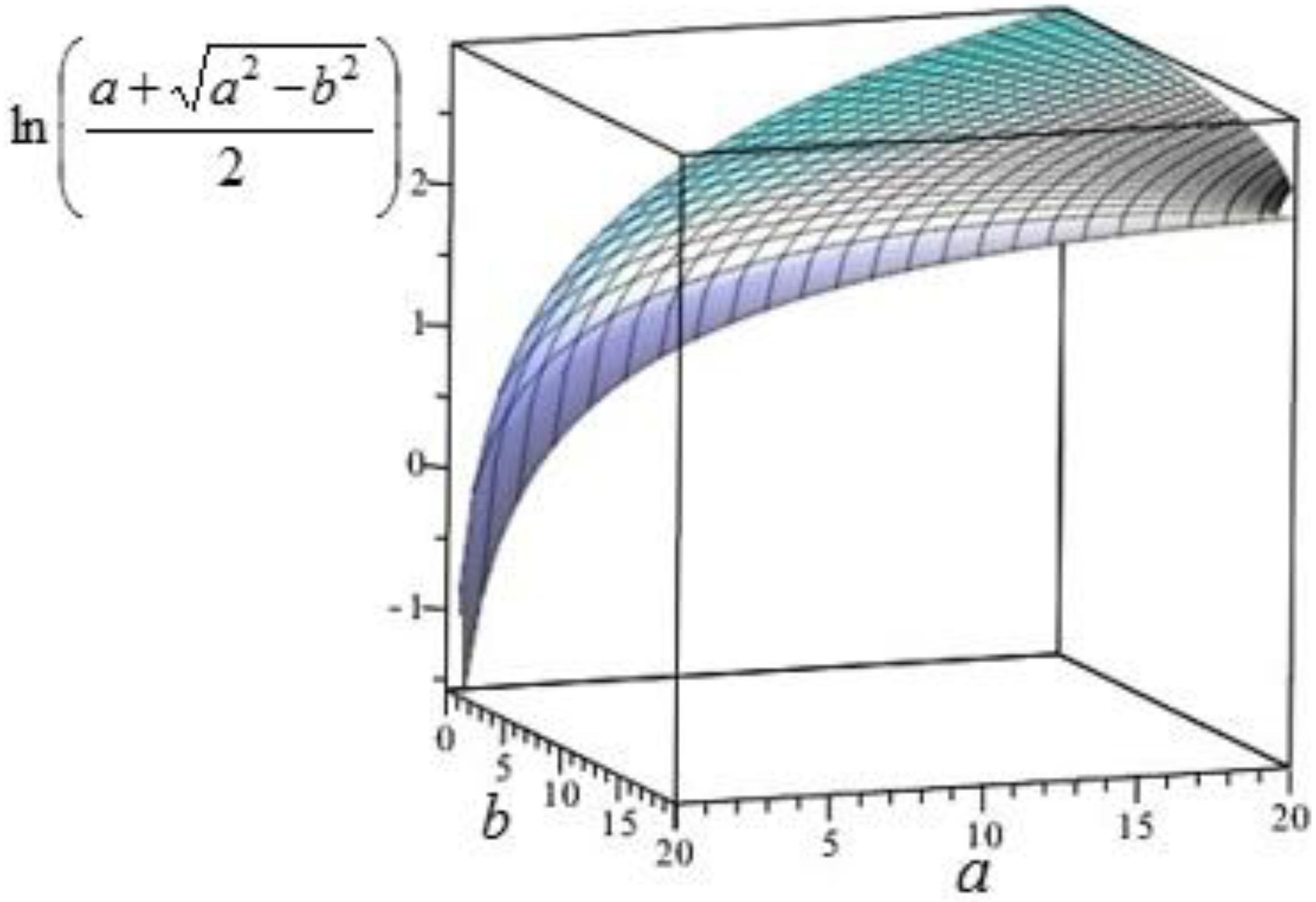
The energy is conserved since we have adiabatic boundaries and, thus:
and the exergy is given by:
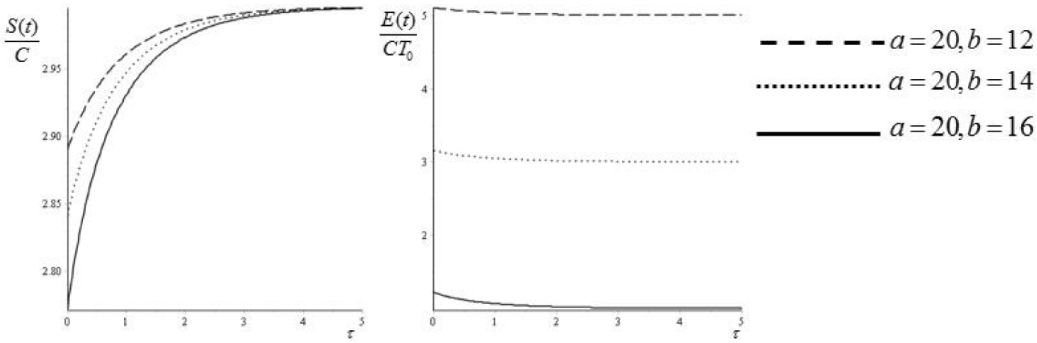
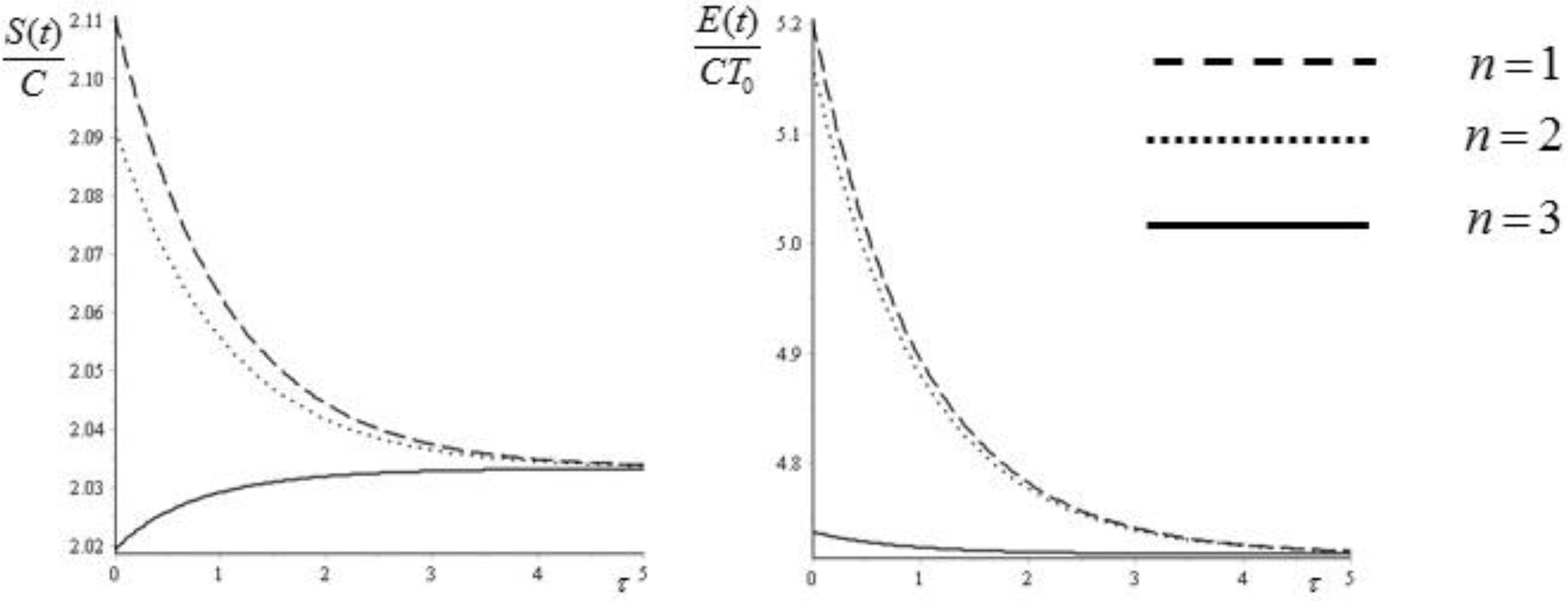
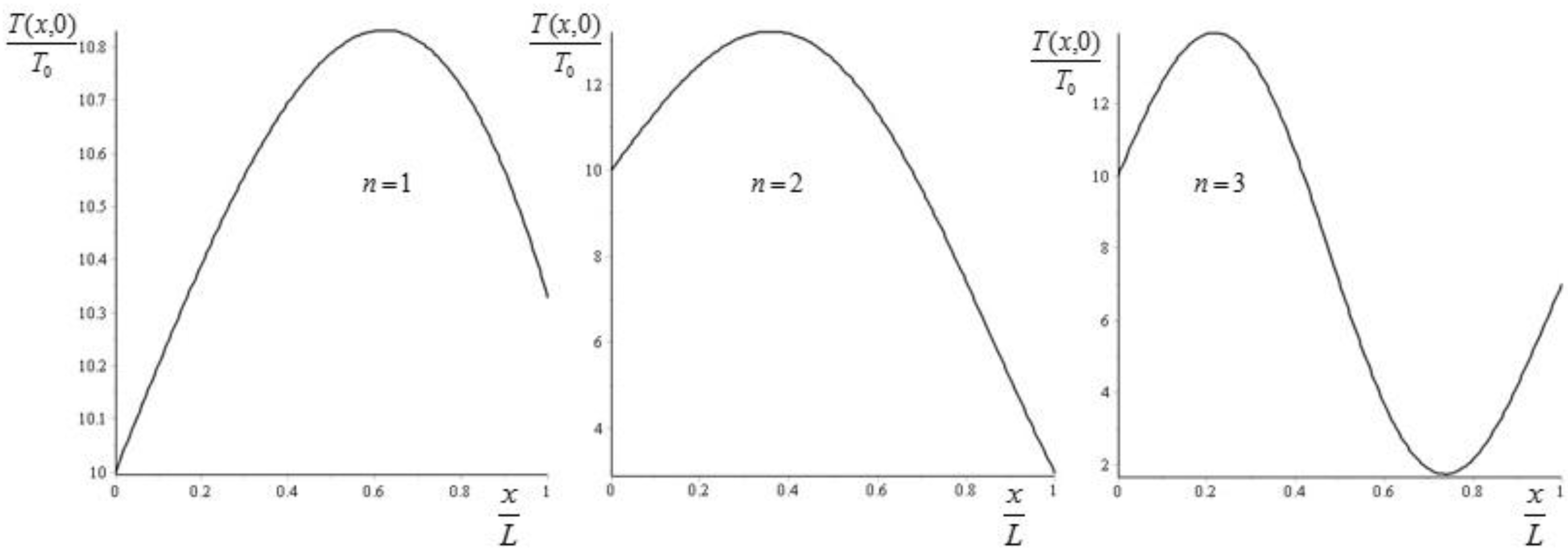
From Equation (45) we see that adding more crests to the initial condition forces the system to a faster approach to equilibrium. If we take and , then we can plot the values of for , corresponding to (see Figure 2).
The values of are then obtained by moving towards (since the exponential term relaxes very fast). It follows then that increases exponentially from the value to the value . Some specific examples are given in Figure 3.
The next example is a bar having the extreme at at a constant temperature, say equal to . The other extreme, at , can exchange heat by convection. The evolution of the temperature is explicitly described by:
where is the Biot number associated with the extreme at x = L exchanging energy via convection and the are the Fourier eigenvalues given by the roots of the transcendental equation . The Fourier coefficients are given by the following integrals:
As initial condition we take the stationary state plus the nth Fourier mode, i.e.,:
The evolution of temperature is described by:
8. Discussion
The general procedure adopted in this study was that of deriving the evolution of the thermal field within a system initially in thermal non-equilibrium, by analytically solving the applicable diffusion equation. Four quantities are of interest in the present context:
- (1)
- The Gibbs’ available energy , defined as the double integral of the quantity from to and from t = 0 to t = ∞, when the system has reached its adiabatic internal equilibrium at Teq;
- (2)
- The classical equilibrium exergy , defined as the double integral of the quantity from to and from t = 0 to t = ∞;
- (3)
- The non-equilibrium exergy , defined as the double integral of the quantity from to and from t = 0 to t = ∞.
- (4)
- The non-equilibrium entropy , defined by Equation (1).
The first conclusion follows from the very definitions of each quantity: A, Eeq and En−eq attain different values, as expected. As for the Sn−eq, it also follows from its definition that, since the initial energy level is known and the non-equilibrium exergy can be calculated at each instant of time, a non-equilibrium entropy can be defined for any system as , its value depending, as predicted, both on the boundary conditions and on the initial T profile. Correspondingly, for each initial temperature -and for a given set of boundary conditions- the initial entropy of the non-equilibrium system is . The original Gibbs entropy/energy plane may thus be extended into a 3-D representation, in which each point in the “non-equilibrium” zone (that obviously corresponds in our model to a different temperature distribution) is identified by a different non-equilibrium exergy value. Iso-energetic initial states may have very different entropy “content”, the exact value depending essentially on the degree of non-uniformity of the initial energy distribution. A higher disuniformity leads to a faster relaxation of the entropy. This is analogous to the Tsallis’ entropy. Given a certain number k of initial subdomains and a level of the initial energy , we may consider every temperature distribution as a randomly assigned energy allocation over a number k of possible “cells”. Each one of these allocations can be assigned a single value of the non-equilibrium entropy , but the reverse is not true, in that any S(t0) may correspond to an infinite number of allocations of . Tsallis’ “correlation parameter” q may be seen as an “indicator” attached to every distribution : given , q is known, but the reverse is not true. Notice that, when the initial energy is equidistributed, S(t0) is equal to its equilibrium value, as is Tsallis’ entropy for q = 0; and that in the limit of infinitely small δx (k → ∞), each distribution tends to a finite limit Sn-eq calculated here as does Tsallis’ entropy for ∀q (This analogy must be taken with care. We are assuming here that the k domains represent the possible states among which the T(t0,x) can be distributed. While it is correct to imagine that the energy can be allocated randomly among these states, there is no logical implication that the probabilities of the allocation (a) are not correlated and (b) sum to unity. Thus, the analogy is non complete from a formal point of view).
The non-equilibrium entropy depends not only on the energy level, but on the initial energy distribution, and therefore it is a multi-valued function: thus, the conclusion by Lieb and Yngvason (“it is generally not possible to find a unique entropy that has all relevant physical properties” [3]) is confirmed, but our method demonstrates that this objection, while true, can be circumvented if we accept a multi-valued entropy.
Finally, our method embeds, so to say, a weaker form of the multi-level approach by Grmela et al. [2]. The nature and distribution of the spatial subdomains k was not specified here, the only assumption being that their number is sufficiently large. It is clear though that an increase of k corresponds to the analysis being applied to a “lower level” in Grmela’s sense, as long as, of course, the local equilibrium hypothesis is applicable. In the limit k → ∞, if the phenomenological conditions are such that local equilibrium is no longer applicable, non-local effects (like those accounted for by the Cattaneo equation, for instance) may be included in the calculation of the non-equilibrium exergy, and suitable formulae can still be derived with a degree of approximation depending only on the accuracy of the adopted correlations. Notice that the GENERIC formalism [33] postulates the existence of a modified Ginzburg-Landau Hamiltonian, consisting of an operator L applied to the reversible part of the process and a “dissipative operator” M applied to the entropic portion. The two operators are linked by certain well-defined rules. Our work stems from a different application of the Ginzburg-Landau assumption that avoids the use of two different operators and adopts exergy as the “non-equilibrium potential”, i.e., as the potential that is driving the system towards equilibrium, under the “driving forces” established—problem by problem—by the boundary and initial conditions
9. Conclusions
A quantity exists called the non-equilibrium entropy, the very existence of which is negated by classical Thermodynamics. This quantity can be univocally calculated for any system once the non-equilibrium energy U(t) and the corresponding non-equilibrium exergy E(t) during the relaxation from non-equilibrium to equilibrium are calculated. U is exactly known once the system initial state is completely (in the sense discussed above) described, and E can be calculated if, additionally, a reference “reservoir” is defined. Under quite simple assumptions that apply to most macroscopic systems of engineering interest, S(t) assumes different values for iso-energetic initial non-equilibrium states that display different distributions of intensive variables (e.g., temperature, pressure or concentration). A visual representation of the state of affairs can be obtained by extending the Gyftopoulos-Beretta S/U plane into a third dimension: in the 3D space S/U/E, only along the equilibrium line is Seq a single-valued function of U. At any non-equilibrium point in the state space, where for a certain U different Enon-eq may correspond because of the internal dishomogeneity of the system, there are as many Snon-eq values as there are Enon-eq. Thus, to each initial internal distribution there corresponds a unique and exactly computable value of Snon-eq, and all of these Snon-eq have Seq as their upper bound. It is also possible to derive an equation for the evolution of the Snon-eq to Seq, i.e., for the relaxation of a system to equilibrium. The results presented here are derived under a local equilibrium assumption and via an explicit time integration, and therefore do not necessarily apply when the smaller space- or timescales of the dishomogeneities are such that such assumption is not applicable, like in explosions, ablation, highly exothermic chemical reactions and the like.
Author Contributions
Enrico Sciubba and Federico Zullo contributed equally to this work.
Conflicts of Interest
The authors declare no conflict of interest.
List of Symbols
| Entity and Units | Symbol |
| Availability, J/kg, J | a,A |
| Density, kg/m3 | ρ |
| Coordinate | x |
| Energy, J/kg, J | u,U |
| Entropy, J/(kg·K), J/K | s,S |
| Exergy, J/kg, J | e,E |
| Mass, kg | M |
| Mass density, kg/m, kg/m2 | m |
| Rod length, m | L |
| Specific heat, J/(kg·K) | c |
| Temperature, K | T |
| Temperature scaling factor, T1/T0 | w |
| Time, s | t |
| Volume, m3 | V |
References
- Tsallis, C. 1988: Possible generalization of Boltzmann–Gibbs statistics. J. Stat. Phys. 1988, 52, 479–487. [Google Scholar] [CrossRef]
- Grmela, M.; Grazzini, G.; Lucia, U.; Yahia, L.H. Multiscale Mesoscopic Entropy of Driven Macroscopic Systems. Entropy 2013, 15, 5053–5064. [Google Scholar] [CrossRef]
- Lieb, E.H.; Yngvason, J. The entropy concept for non-equilibrium states. Proc. R. Soc. A 2013, 469, 2158. [Google Scholar] [CrossRef] [PubMed]
- Demirel, Y. Nonequilibrium thermodynamics modeling of coupled biochemical cycles in living cells. J. Non-Newtonian Fluid Mech. 2010, 165, 953–972. [Google Scholar] [CrossRef]
- Prigogine, I. Introduction to Thermodynamics of Irreversible Processes; Interscience Pub.: New York, NY, USA, 1955. [Google Scholar]
- Kleidon, A. A basic introduction to the thermodynamics of the Earth. Philos. Trans. R. Soc. Lond. B Biol. Sci. 2010, 365, 1303–1315. [Google Scholar] [CrossRef] [PubMed]
- Dewulf, J.; Langenhove, H.; Muys, B.; Bruers, S.; Bakshi, B.; Grubb, G.; Paulus, D.; Sciubba, E. Exergy: its potential and limitations in environmental science and technology. Environ. Sci. Technol. 2008, 42, 2221–2232. [Google Scholar] [CrossRef] [PubMed]
- Grubbström, R.W. An attempt to introduce dynamics into generalized exergy considerations. Appl. Energy 2007, 84, 701–718. [Google Scholar] [CrossRef]
- Grubbström, R.W. On the Exergy Content of an Isolated Body in Thermodynamic Disequilibrium. Int. J. Energy Optim. Eng. 2012, 1, 1–18. [Google Scholar] [CrossRef]
- Jörgensen, S.E.; Fath, B.D. Fundamentals of Ecological Modelling; Elsevier: Amsterdam, The Netherlands, 2001. [Google Scholar]
- Li, G.; von Spakovsky, M.R. Study of Nonequilibrium Size and Concentration Effects on the Heat and Mass Diffusion of Indistinguishable Particles using Steepest-Entropy-Ascent Quantum Thermodynamics. J. Heat Transfer 2017, 139, 122003. [Google Scholar] [CrossRef]
- Sciubba, E. Do the Navier-Stokes Equations Admit of a Variational Formulation? In Variational and Extremum Principles in Macroscopic Systems; Sieniutycz, S., Farkas, H., Eds.; Elsevier: Amsterdam, The Netherlands, 2005. [Google Scholar]
- Barbera, E. On the principle of minimal entropy production for Navier-Stokes-Fourier fluids. Contin. Mech. Thermodyn. 1999, 11, 327–330. [Google Scholar] [CrossRef]
- Sciubba, E.; Zullo, F. Exergy Dynamics of Systems in Thermal or Concentration Non-Equilibrium. Entropy 2017, 19, 263. [Google Scholar] [CrossRef]
- Hatsopoulos, G.N.; Gyftopoulos, E.P. A Unified Quantum Theory of Mechanics and Thermodynamics. Part I: Postulates. Found. Phys. 1976, 6, 15–31. [Google Scholar] [CrossRef]
- Hatsopoulos, G.N.; Gyftopoulos, E.P. A Unified Quantum Theory of Mechanics and Thermodynamics. Part IIa: Available Energy. Found. Phys. 1976, 6, 127–141. [Google Scholar] [CrossRef]
- Hatsopoulos, G.N.; Gyftopoulos, E.P. A Unified Quantum Theory of Mechanics and Thermodynamics. Part IIb: Stable Equilibrium States. Found. Phys. 1976, 6, 439–455. [Google Scholar] [CrossRef]
- Gyftopolous, E.P.; Beretta, G.P. Thermodynamics: Foundations and Applications; Macmillan Pub.: London, UK, 1991. [Google Scholar]
- Beretta, G.P. Axiomatic Definition of Entropy for Nonequilibrium States. Int. J. Thermodyn. 2008, 11, 39–48. [Google Scholar]
- Gaggioli, R.A. Teaching elementary thermodynamics and energy conversion: Opinions. Energy 2010, 35, 1047–1056. [Google Scholar] [CrossRef]
- Gaggioli, R.A.; Richardson, D.H.; Bowman, A.J. Available Energy—Part I: Gibbs revisited. J. Energy Resour. Technol. 2002, 124, 105–109. [Google Scholar] [CrossRef]
- Gaggioli, R.A.; Paulus, D.M. Available Energy—Part II: Gibbs extended. J. Energy Resour. Technol. 2002, 124, 110–115. [Google Scholar] [CrossRef]
- Cimmelli, V.A.; Jou, D.; Ruggeri, T.; Ván, P. Entropy Principle and Recent Results in Non-Equilibrium Theories. Entropy 2014, 16, 1756–1807. [Google Scholar] [CrossRef]
- Gyarmati, I.; Gyarmati, E. Non-Equilibrium Thermodynamics; Springer: Berlin, Germany, 1970. [Google Scholar]
- Lebon, G.; Jou, D.; Casas-Vazquez, J. Understanding Non-Equilibrium Thermodynamics; Springer: New York, NY, USA, 2008. [Google Scholar]
- Beretta, G.P.; Gyftopoulos, E.P.; Park, J.L. Quantum thermodynamics. A new equation of motion for a general quantum system. IL Nuovo Cimento B 1985, 87, 77–97. [Google Scholar] [CrossRef]
- Zanchini, E.; Beretta, G.P. Recent Progress in the Definition of Thermodynamic Entropy. Entropy 2014, 16, 1547–1570. [Google Scholar] [CrossRef]
- Kotas, T.J. Teaching the Exergy Methods to Engineers. In Teaching Thermodynamics; Levins, J., Ed.; Plenum Press: Berlin, Germany, 1986; pp. 373–385. [Google Scholar]
- Gibbs, J.W. 1875: On the Equilibrium of Heterogeneous Substances. In The Scientific Papers of J.W. Gibbs; Dover Publications: New York, NY, USA, 1961; Volume 1. [Google Scholar]
- Straughan, B. A note on convection with nonlinear heat flux. Ricerche Mat. 2007, 56, 229–239. [Google Scholar] [CrossRef]
- Zullo, F. Entropy Production in the Theory of Heat Conduction in Solids. Entropy 2016, 18, 87. [Google Scholar] [CrossRef]
- Gradshtein, I.S.; Ryzhik, I.M. Table of Integrals, Series and Products; Elsevier: Amsterdam, The Netherlands, 2007. [Google Scholar]
- Grmela, M.; Öttinger, H.C. Dynamics and thermodynamics of complex fluids. I. Development of a general formalism. Phys. Rev. E 1997, 56, 6620. [Google Scholar] [CrossRef]
Figure 1.
The extension of the Gibbs entropy/energy plane to non-equilibrium cases: the plane shown is described by and contains the orbits of the system, i.e., its evolution lines for different values of .
Figure 1.
The extension of the Gibbs entropy/energy plane to non-equilibrium cases: the plane shown is described by and contains the orbits of the system, i.e., its evolution lines for different values of .
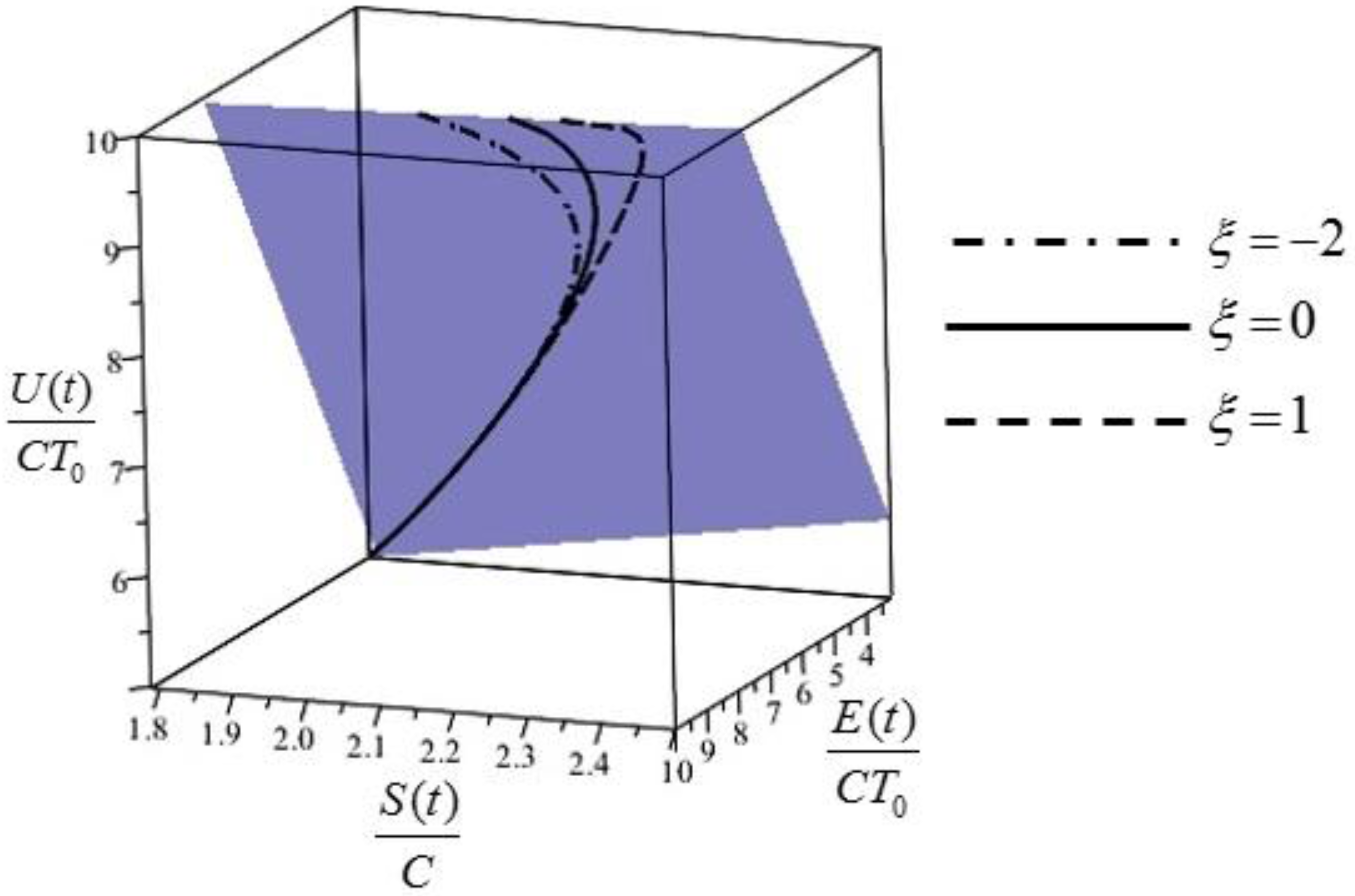
Figure 2.
Plot of for , corresponding to for the initial condition (43). The values of are obtained by moving towards .
Figure 2.
Plot of for , corresponding to for the initial condition (43). The values of are obtained by moving towards .

Figure 3.
Entropy (45) and exergy (47) as functions of the dimensionless time for three different pairs of values (a, b).
Figure 3.
Entropy (45) and exergy (47) as functions of the dimensionless time for three different pairs of values (a, b).

Figure 4.
Entropy (45) and exergy (47) as functions of the dimensionless time . The values of the temperatures are and .
Figure 4.
Entropy (45) and exergy (47) as functions of the dimensionless time . The values of the temperatures are and .

Figure 5.
The initial condition (50) corresponding to the plots in Figure 4.
Figure 5.
The initial condition (50) corresponding to the plots in Figure 4.
© 2017 by the authors. Licensee MDPI, Basel, Switzerland. This article is an open access article distributed under the terms and conditions of the Creative Commons Attribution (CC BY) license (http://creativecommons.org/licenses/by/4.0/).
Share and Cite
MDPI and ACS Style
Sciubba, E.; Zullo, F. A Novel Derivation of the Time Evolution of the Entropy for Macroscopic Systems in Thermal Non-Equilibrium. Entropy 2017, 19, 594. https://doi.org/10.3390/e19110594
AMA Style
Sciubba E, Zullo F. A Novel Derivation of the Time Evolution of the Entropy for Macroscopic Systems in Thermal Non-Equilibrium. Entropy. 2017; 19(11):594. https://doi.org/10.3390/e19110594
Chicago/Turabian StyleSciubba, Enrico, and Federico Zullo. 2017. "A Novel Derivation of the Time Evolution of the Entropy for Macroscopic Systems in Thermal Non-Equilibrium" Entropy 19, no. 11: 594. https://doi.org/10.3390/e19110594
Note that from the first issue of 2016, this journal uses article numbers instead of page numbers. See further details here.