Comparison of Two Entropy Spectral Analysis Methods for Streamflow Forecasting in Northwest China

1
College of Water Resources and Architectural Engineering, Northwest A&F University, Yangling 712100, China
2
Department of Biological & Agricultural Engineering and Zachry Department of Civil Engineering, Texas A&M University, 2117 TAMU, College Station, TX 77843, USA
*
Author to whom correspondence should be addressed.
Entropy 2017, 19(11), 597; https://doi.org/10.3390/e19110597
Submission received: 27 September 2017
/
Revised: 1 November 2017
/
Accepted: 5 November 2017
/
Published: 7 November 2017
(This article belongs to the Special Issue Entropy Applications in Environmental and Water Engineering)
Abstract
:Monthly streamflow has elements of stochasticity, seasonality, and periodicity. Spectral analysis and time series analysis can, respectively, be employed to characterize the periodical pattern and the stochastic pattern. Both Burg entropy spectral analysis (BESA) and configurational entropy spectral analysis (CESA) combine spectral analysis and time series analysis. This study compared the predictive performances of BESA and CESA for monthly streamflow forecasting in six basins in Northwest China. Four criteria were selected to evaluate the performances of these two entropy spectral analyses: relative error (RE), root mean square error (RMSE), coefficient of determination (R2), and Nash–Sutcliffe efficiency coefficient (NSE). It was found that in Northwest China, both BESA and CESA forecasted monthly streamflow well with strong correlation. The forecast accuracy of BESA is higher than CESA. For the streamflow with weak correlation, the conclusion is the opposite.
1. Introduction
Accurate streamflow forecasting is important for developing measures to flood control, river training, navigation, reservoir operation, hydropower generation plan and water resources management. Time series models, such as autoregressive (AR) or autoregressive moving average (ARMA) models, as proposed by Box and Jenkins [1], are generally used for monthly streamflow forecasting [2,3,4]. These models assume that streamflow time series is stochastic and are linear which limits their application [5]. Monthly streamflow time series not only exhibits stochastic characteristics but also seasonal and periodic patterns. Entropy spectral analysis can extract important information of time series, such as the periodic characteristics [6,7,8,9,10,11]. Therefore, combining entropy spectral theory with time series analysis provides a new way for streamflow forecasting. Considering frequency f as a random variable, Burg [12] defined entropy, called Burg entropy, and developed an algorithm for the estimation of spectral density function of time series using the principle of maximum entropy (POME). The algorithm is termed Burg entropy spectral analysis (BESA) and has been widely used for spectral analysis of geomagnetic series [13], climate indices [8,14], surface air temperature [15], tide levels [16], precipitation and runoff series [17], and flood stage [18]. BESA is recommended as better than traditional methods for long-term hydrological forecasting [19,20,21,22,23]. Huo et al. [24] applied BESA to simulate and predict groundwater in the west of Shandong province plain of the Yellow River downstream and achieved satisfactory results. Wang and Zhu [25] considered that implicit periodic components of monthly and annual hydrological time series were better identified by BESA. Shen et al. [26] proposed a more rigorous recursion algorithm for maximum entropy spectral estimation method. In addition to meeting forward and backward minimum error of BESA, the algorithm also needed to satisfy a condition that the optimal prediction error was orthogonal to the signal. It was considered that the spectral density resolution of this method was higher than that of BESA. Boshnakov and Lambert-Lacroix [27] proposed an extension of the periodic Levinson-Durbin algorithm which was considered more reliable. However, multi-peak spectral density is difficult to determine under non-stationary conditions. Hence, monthly streamflow that features strong seasonal and periodic characteristics cannot be well simulated [28].
Frieden [29] was the first to use configurational entropy in image reconstruction and Gull and Daniell [30] applied it to radio astronomy. Based on the finite length cepstrum model, Wu [31] deduced an explicit spectral density function estimation formula and solved the complex calculation problem of CESA. Nadeu [32] regarded that spectral estimation precision of CESA was higher than that of BESA for both ARMA and MA, while the corresponding precisions were quite similar for AR. Katsakos et al. [33] found that the precision was higher when the spectral density of white noise series was estimated. Based on the spectral density estimation formula constructed by Wu, Cui, and Singh [28] derived a single variable streamflow forecasting model and found that the forecasting accuracy of CESA was superior to BESA for 19 different rivers in the US. For monthly streamflow forecasting, resolution and reliability of CESA were better than those of BESA.
The objective of this paper therefore was to compare the forecast performances of BESA and CESA for monthly streamflow forecasting in Northwestern China. The paper is organized as follows. First, a brief introduction to streamflow forecasting is given. Second, a maximum entropy spectral analysis prediction model is derived and evaluation methods are discussed. Third, application to streamflow forecasting is discussed. Fourth, results are discussed. Finally, conclusions were given.
2. Derivation and Evaluation of Maximum Entropy Spectral Analysis Prediction Model
2.1. Maximum Entropy Model
Let streamflow time series frequency f be a random variable, and the normalized spectral density P(f) be taken as the probability density function. Thus, the Burg entropy can be defined as
The configurational entropy is defined in the same form as the Shannon entropy and can be written as
where W = 1/(2Δt) is the Nyquist fold-over frequency and f is the frequency that varies from −W to W, Δt is the sampling period, P(f) is the normalized spectral density of streamflow series.
2.2. Constraints for Model
For a given streamflow time series, the constraints can be formed from the relationship between the spectral density P(f) and autocorrelation function ρ(n), which can be written as
where Δt is the discretization or sampling interval, and . N is normally taken from ¼ up to ½ of the series length according to the periodicity of streamflow.
2.3. Determination of Spectral Density
To obtain the least biased spectral density P(f) by entropy maximizing, one needs to maximize the Burg and configurational entropies. Entropy maximizing can be done by using the method of Lagrange multipliers in which the Lagrangian function for the Burg entropy and configurational entropies can be formulated as follows:
where λn, n = 0, 1, 2, …, N, are the Lagrange multipliers. Taking the partial derivative of Equations (4) and (5) with respect to P(f) and equating the derivative to zero, the least-biased spectral densities P(f) obtained from the maximization of the Burg entropy and configurational entropy, respectively, are
It can be seen from the above two equations that the spectral density derived from the Burg entropy is in the form of inverse of polynomials, while the one from the configurational entropy is in the exponential form, which is easier to manipulate. The form in Equation (6) suggests that BESA is related to a linear prediction process.
2.4. Solution of the BESA Model
The spectral density derived is defined in the same form as the autoregressive model. On the basis of minimum of the forward and backward prediction error, a method of parameter estimation was presented by Burg, which can be written as
where is the i-th parameter value of the k-order autoregressive model, and the parameter is estimated by minimizing the forward and backward prediction error.
where , x(t) is the streamflow time series.
For configurational entropy, the Lagrange multipliers and the extension of autocorrelation function can be computed by cepstrum analysis. Then, Wu [31] deduced the explicit solution based on the maximization of configurational entropy. Taking the inverse Fourier transform of the log-magnitude of Equation (7), it becomes
where the second part of the left side of Equation (10) can be denoted as
Doing the integration of both sides of Equation (10), one gets
where δn is the Dirac delta function defined as
Equation (12) can be expanded as a set of N linear equations:
Equation (14) shows that the Lagrange multipliers can be determined from the values of cepstrum which entails the spectral density that is obtained from Equation (7). It is the main difference from Burg entropy.
For convenience of solving for the spectral density function, Nadeu [32] developed a simple method for computing cepstrum based on the use of the causal part of autocorrelation, where ρ(n) is used only for −N ≤ n ≤ N. Thus, cepstrum can be estimated by the following recursive relation:
On the other hand, for the configurational entropy, the autocorrelation is extended with the inverse relationship of Equation (15) using the autocepstrum as
Therefore, with model order m determined, the autocorrelation function can be estimated as
with extension coefficients , and m is the model order.
Equation (17) extends the autocorrelation function with the configurational entropy maximized. Surprisingly, the autocorrelation extends with a linear combination of past lags, which is the same with the Burg entropy or the AR method. Thus, Equation (17) can be also written as
where T is the total time period.
The extended autocorrelation in Equation (18) is a linear combination of the previous values weighted with coefficients . Burg (1975) suggested weighing time series using the extension coefficients as
2.5. Determination of Model Order
The order of forecasting model m is identified by the Bayesian Information Criterion (BIC) [34]. BIC can reduce the order of the model by penalizing free parameters more strongly compared with AIC (Akaike information criterion).
where N is the length of time series and is the variance of residual.
2.6. Procedure for Streamflow Forecasting
The computation procedure for monthly streamflow forecasting is shown in Figure 1. The computation steps are as follows: (1) Streamflow data x(t) are normalized with Equation (21); (2) The parameters in the model (BESA and CESA) are estimated and the cepstrum values are determined for computing the Lagrange multipliers; (3) The forecast order m is identified by the Bayesian Information Criterion (BIC) and monthly streamflow is forecasted; (4) The prediction results of streamflow series are obtained by inverse normalization and exponential transformation.
where zscore is a standardized function and y(t) is a logarithmic sequence minus the mean divided by the standard deviation of the original sequence.
2.7. Evaluation of Model Forecast Performances
Four criteria were selected to evaluate the prediction model performance: relative error (RE), root mean square error (RMSE), coefficient of determination (R2), and Nash–Sutcliffe efficiency coefficient (NSE). The relative error provides the average magnitude of differences between observed values and predicted values relative to observed values. RMSE also represents the difference between observed and predicted values, however, it is scale-dependent. The coefficient of determination is defined as the square of the coefficient of correlation. It ranges between 0 and 1, and its higher values indicate better prediction. The Nash–Sutcliffe efficiency coefficient, defined by Nash and Sutcliffe [35], ranges from negative infinity to 1. Higher values of NSE represent more agreement between model predictions and observations, and negative values indicate that the model is worse than the mean value as a predictor.
where N is the number of observed streamflow data, Qo(i) is the i-th observed streamflow, Qf(i) is the i-th forecasted streamflow, and are the average values of observed and forecasted streamflow, respectively.
3. Application to Streamflow Forecasting
3.1. Observed Data and Characteristics
The two entropy spectral analysis methods, BESA and CESA, were testedusing observed streamflow data from six river sites on the Yellow River, Heihe River, Zamu River, Xiying River, Datong River, and Daxia River. The Yellow River has a large drainage area of 752,443 km2, with an average monthly streamflow of 633 m3/s. Datong River and Daxia River are tributaries of the Yellow River. These two rivers have drainage areas of 151,33 km2 and 7154 km2, with average monthly streamflow of 88 m3/s and 27 m3/s, respectively. Zamu River and Xiying River belong to the Shiyang River watershed, with drainage areas of 851 km2 and 1120 km2. The Heihe River is the second largest interior river in Northwest China, with a drainage area of 130,000 km2. Six hydrological stations selected in this paper are located in the Yellow River, Heihe River and Shiyang River, respectively. Tangnaihai station is located on the mainstream of Yellow River, while Xiangtang and Zheqiao stations are located on the tributary of Yellow River, Zamusi and Jiutiaoling stations are situated on the Shiyang River. Yingluoxia station is located in the Heihe River and it marks the boundary between the upstream and middle reaches. The location and basic information of each station are shown in Figure 2 and Table 1.
Monthly streamflow box-plots with all available data are presented in Figure 3. The bottom (Q1) and top (Q3) of the box are the first and third quartiles of streamflow, and the band inside the box is the median of streamflow. The inter quartile range (IQR) is equal to the difference between first and third quartiles. The limit of whiskers is called the inner fence which is 1.5 IQR from the quartile and the outer fence is 3 IQR from the quartile. Outliers are points that fall outside the limits of whiskers. + represents mild outliers which are between an inner and outer fence. × represents the extreme outliers which are beyond one of the outer fences. As shown in Figure 3, streamflow is concentrated during the flood season (June–September), and it drops down in the non-flood season. Because precipitation is the most important streamflow supply and the precipitation in these basins is concentrated during June–September.
There are many mild and extreme outliers for monthly streamflow data during the flood season at Xiangtang and Zheqiao stations, respectively. This is mainly due to poor vegetation coverage and barren hills in Datong River (Xiangtang station) downstream regions. Meanwhile, rainfall is mainly concentrated from June to September and mainly consists of heavy rain. Daxia River (Zheqiao station) upstream and downstream flow through the rocky mountainous region and loess plateau, separately. Serious soil erosion, heavy rain, mudslides, and landslides are frequent there. Streamflow during the flood season has many positive outliers for every station (Figure 3), and logarithmic processing is able to reduce the skewness of positive outliers in Section 2.7.
3.2. Comparison the Results of BESA and CESA
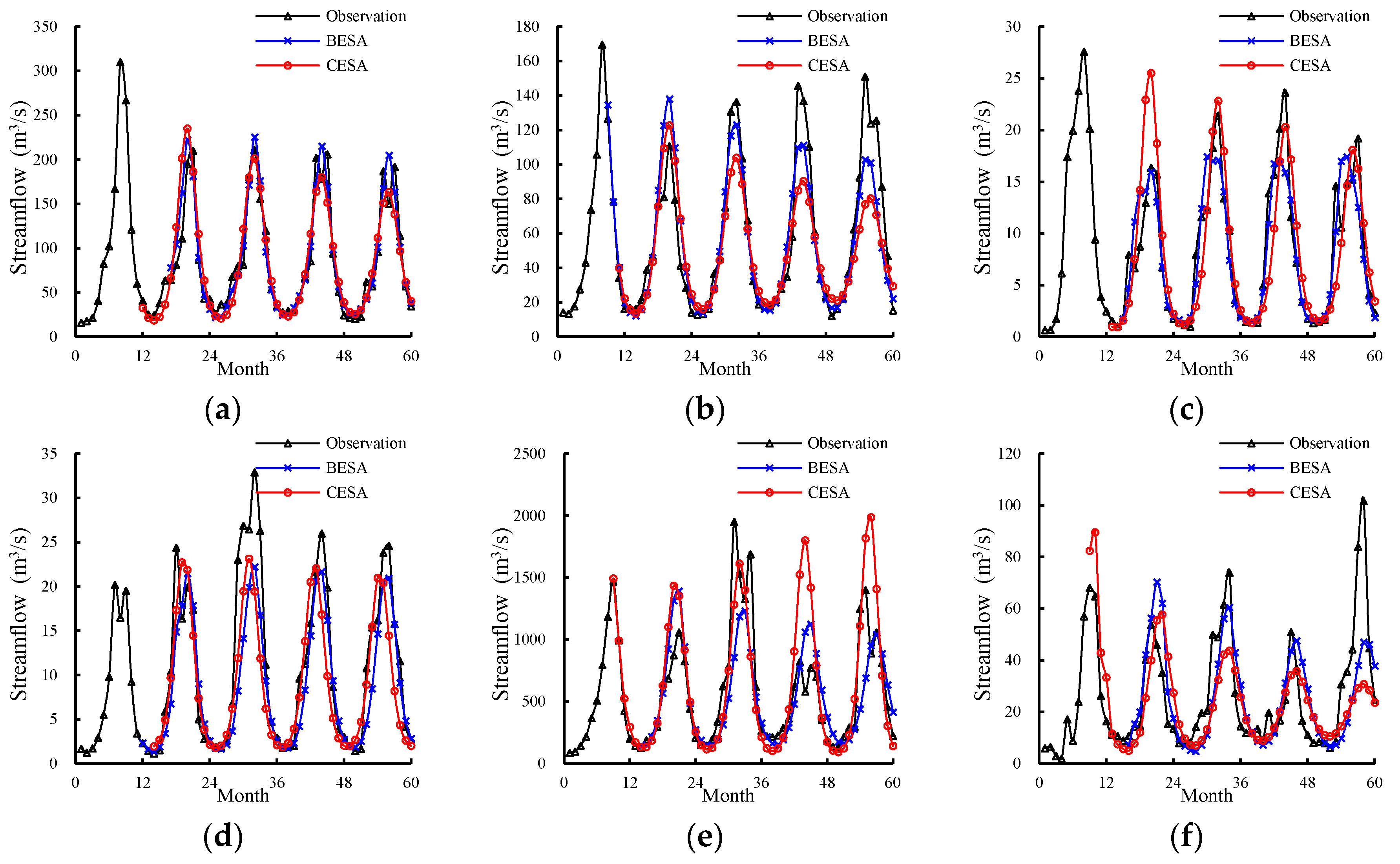
It is shown in a previous study that with the increase of the training time, both the accuracy of the training time and the precision of the lead time do not increase. Streamflow is forecasted by the two entropy spectral analysis methods with a five year training time (2003–2007) and a three year lead time (2008–2010) for representative stations. The simulated values and observed values for the two entropy spectrum models during the training period are shown in Figure 4. Both models were capable of simulating preferably streamflow variations at all stations. However, simulation results were better for the short leading time than that of the long leading time. The error between observed and simulated values was increasing with the lead time extension. The simulation values were better in drought seasons than in flood seasons, which mainly reflected the peak position and peak values. The maximum discharge during the flood seasons for six rivers appeared in different months for every year. This may lead to one month in advance or delay for the simulated values than the observed values for both methods. The predicted streamflow in the flood seasons was lower than observed streamflow for some stations. It was mostly at Yingluoxia, Tangnaihai and Zheqiao stations. Compared with CESA, the predicted and observed values were closer in flood seasons for BESA model. Overall, the simulation of streamflow time series at the above stations was superior for BESA to CESA.
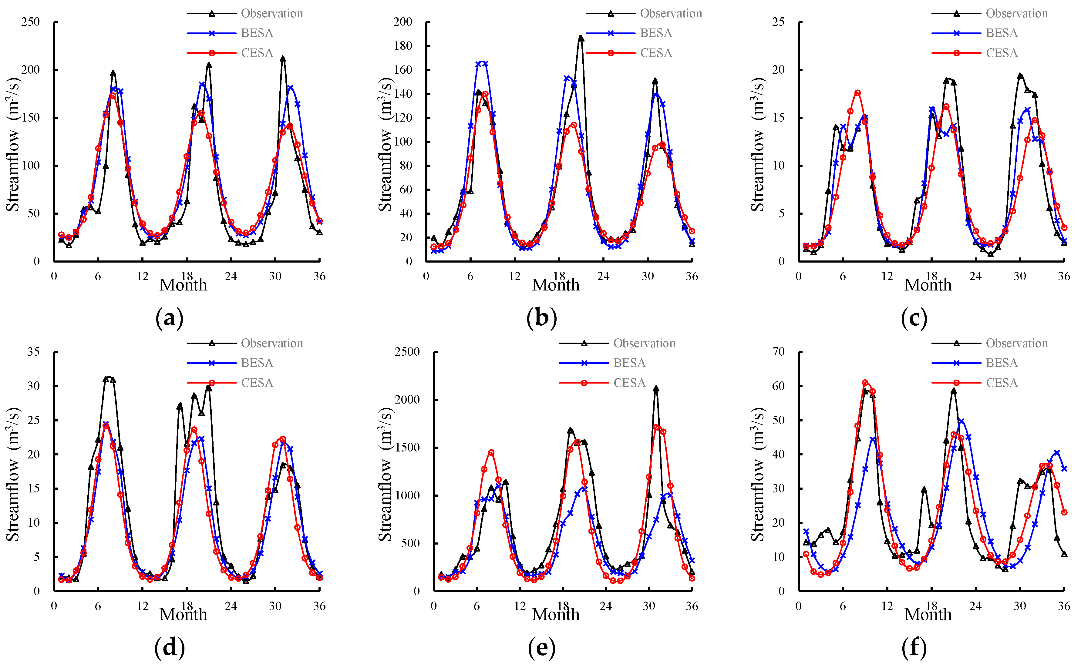
The forecasted values and observed values for two entropy spectral models in the lead time are shown in Figure 5. For Xiangtang, Yingluoxia, Zamusi, and Jiutiaoling stations, both models satisfactorily forecasted streamflow. In the first lead year, two models accurately forecasted the time of maximum monthly streamflow at Xiangtang, Yingluoxia, and Jiutiaoling stations. Nevertheless, the predicted maximum streamflow for the last two years appeared one month earlier or later. At Zamusi station, BESA accurately forecasted the bi-modal values of the flood season for the lead time, while CESA did not. BESA forecasted the number of peaks in the following two years, but the peak position appeared one month earlier or later. At Tangnaihai and Zheqiao stations, the difference between the predicted and observed values for BESA model was large. However, CESA still did not forecast the multimodal pattern of partial flood season, while uni-modal year of streamflow in the flood season had better forecast results.
The performance metrics of the models are shown in Table 2. It can be seen that the optimum order of BESA and CESA models range from 8 to 16 and 8 to 13, respectively. The R2 and NSE values at Xiangtang, Yingluoxia, Zamusi, and Jiutiaoling stations during the training period were relatively high, with the values of over 0.86 and 0.70, respectively. The R2 and NSE values at Tangnaihai and Zheqiao stations were lower than at the former four stations. The simulation of streamflow time series during the training period for BESA was better than that of CESA for the former four stations, and performance metrics were superior to CESA. For the other stations, the simulation results were equivalent for the two models. Streamflow forecasting by the two entropy spectrum models was good at Xiangtang, Yingluoxia, Zamusi, and Jiutiaoling stations during the verification period. The corresponding R2 and NSE values were all higher than 0.88 and 0.70, respectively. However, streamflow forecasting at Tangnaihai and Zheqiao stations was relatively poor. Although the R2 values were more than 0.76, the NSE values were between 0.48 and 0.49. BESA performed better at Xiangtang, Yingluoxia, Zamusi, and Jiutiaoling stations while CESA was more suitable for forecasting streamflow at Tangnaihai and Zheqiao stations.
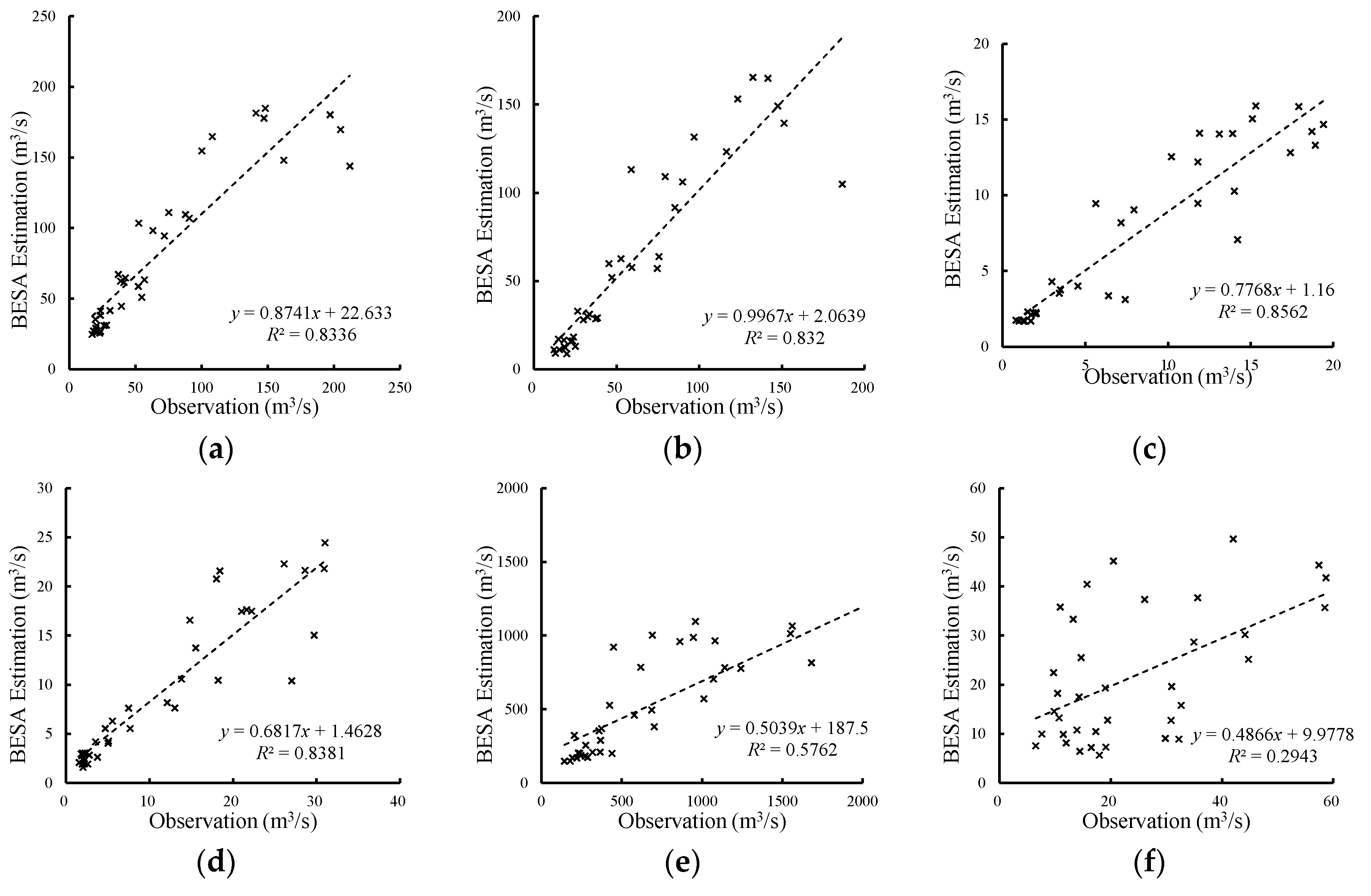
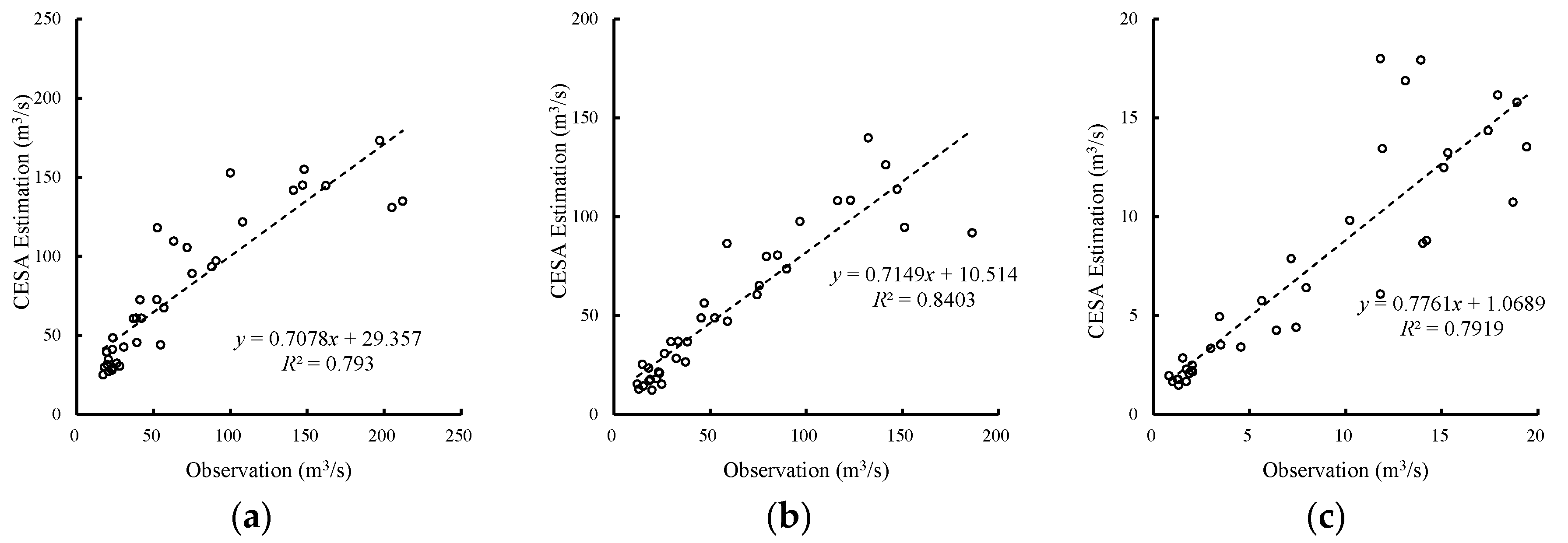
Comparison of monthly streamflow estimated by BESA and CESA and observed values during the verification period is shown in Figure 6 and Figure 7, respectively. The slope of the trend line was closer to 1, indicating that the bias between predicted and observed values was smaller. The larger R2 suggested that the correlation between predicted and observed values was better. That is to say, the predicted values were much closer to the observed values. At Xiangtang, Yingluoxia, Zamusi, and Jiutiaoling stations, the trend line slope of BESA was much closer to 1 than that of CESA and the corresponding R2 was higher. By contrast, the trend line slope of CESA was much closer to 1 than that of BESA at Tangnaihai and Zheqiao stations, and the correlation coefficient was much higher.
Above all, the fitness of BESA for simulating the observed streamflow sequence was better than that of CESA. The forecast accuracy of BESA at Xiangtang, Yingluoxia, Zamusi, and Jiutiaoling stations was better than that of CESA. Nevertheless, it was the opposite at Tangnaihai station. Neither model made better forecasts at Zheqiao station.
3.3. Comparison with Other Autocorrelation Models
The autoregressive coefficients of BESA and CESA are obtained by maximizing Burg entropy and Configurational entropy, respectively. In order to demonstrate the improved accuracy of the predictions, we performed comparison with two other autocorrelation models. The first one is the AR model, and its coefficients are calculated by Yule-Walker function. The second one is the seasonal autoregressive model (SAR), and it rearranges the streamflow by month to avoid the seasonality. The comparison of the performance metrics is shown in Table 3. It can be seen that the BESA and CESA performed better than the AR and SAR models. This is because the BESA and CESA combine the maximum entropy principle and spectral analysis. The model estimated by maximum entropy principle is unbiased with all available data and no further hypothesis are needed. The spectral analysis can detect the periodical pattern of time series. Thus, BESA and CESA is more accurate and reliable than AR and SAR model.
4. Discussion
Despite the fact that the six hydrological stations are in the same area, they differ in factors such as the type of river, control catchment area, vegetation condition, and human activities. Datong River (Xiangtang station), Daxia River (Zheqiao station), and the Yellow River (Yingluoxia station) belong to outflow rivers, whereas Heihe River (Yingluoxia station), Xiying River (Jiutiaoling station), and Zamu River (Zamusi station) belong to interior rivers. As the upstream of Yellow River, the catchment area of Tangnaihai station is the largest, which is about 120,000 km2. Both Xiangtang and Zheqiao stations are located on the tributary of Yellow River, while Zamusi and Jiutiaoling stations are situated on the Shiyang River. Although four hydrological stations are located on the downstream, the catchment area are all less than 20,000 km2. Yingluoxia station is located on the upstream Heihe River, with a catchment area of 10,009 km2. For Xiangtang, Zamusi and Jiutiaoling stations, the upper reaches of piedmont watershed scale have good vegetation coverage and little human activity. By comparison, vegetation coverage is slightly poorer in the middle and lower reaches. Yingluoxia station is located on the Heihe upstream, but its catchment area and vegetation coverage are similar to the upstream of the watershed mentioned above. The impact of human activity is small above Tangnaihai station. In addition, industrial and agricultural water use is rare. Since the 1990s, the grassland has a tendency to gradually degradation. The upstream piedmont of Daxia River (i.e., Zheqiao station-owned) stony mountainous area covered with pasture except for few woods. Its downstream flow through loess plateau with ravines crossbar, poor vegetation and serious soil erosion and concentrated human activities.
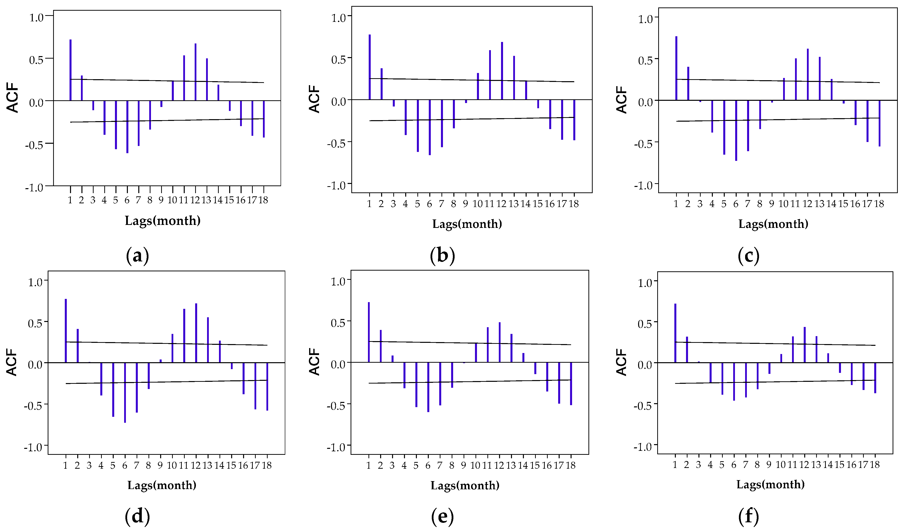
Whether outliers, control catchment area, vegetation condition, and human activities, all reflect correlation of streamflow data. The autocorrelation of the six stations is shown in Figure 8. It can be seen that the autocorrelation of Tangnaihai and Zheqiao stations is relatively low (i.e., the autocorrelation coefficient is less than 0.5 at the 12th lag, and other stations are higher than 0.6). Based on the level of autocorrelation, the six stations can be grouped into two categories. The autocorrelation in the first category (Xiangtang, Yingluoxia, Zamusi, and Jiutiaoling stations) is higher than the second category (Tangnaihai and Zheqiao stations). As streamflow forecasting is based on the autocorrelation with the past series, the streamflow series with strong correlation will be more reliable forecasted. Thus, streamflow forecasting effects of the first category are better than the second category. BESA fitness may be better and unbiased because of the difference methods of the two forecast models. For BESA, the autoregressive coefficients are calculated by Levinson–Burg algorithm, which is developed from the AR model. For CESA, the autoregressive coefficients are calculated by cepstrum estimation. Therefore, entropy spectrum analysis methods need to be chosen carefully according to the situation of the study area.
The six stations selected in this paper are all located in Northwest China. Streamflow is principally composed of precipitation. Precipitation is the main recharge source of streamflow among them. Annual precipitation mainly occurs during June to September. All six rivers originate from alpine regions where April and May are spring flood periods, and flood is mainly formed by snow melt. Although annual precipitation mainly occurs during June to September, rainfall is mostly heavy rain and the month with maximum precipitation is not fixed. Hence, the maximum monthly streamflow is also unset. The input of autoregressive model is only previous monthly streamflow data, which may influence the forecast accuracy of the autoregressive model in the flood season. Therefore, adding precipitation as a predictor, selecting one or more models with high accuracy in the flood season, and using the entropy spectrum model and its combination (such as combined streamflow forecasting based on cross entropy [36]) to forecast can be used as the next research direction.
5. Conclusions
Two entropy spectral analysis methods (Burg entropy and configurational entropy) are mainly developed for streamflow forecasting in Northwest China. The following conclusions are drawn from this study:
- The autoregressive coefficients obtained by maximizing Burg entropy and configurational entropy leads to more reliable than those by Levinson-Durbin algorithm. So, the streamflow forecasted by BESA and CESA is more accurate than that of the AR and SAR models.
- For the streamflow with strong correlation, both BESA and CESA forecast monthly streamflow well. The R2 and NSE were over 0.84 and 0.68, respectively. The forecast accuracy of BESA is higher than that of CESA. For the streamflow with weak correlation, the conclusion is the opposite.
- The time of peak flow forecasted by both models (BESA and CESA) may be either earlier or later than observed. The peak flow is generally underestimated by both models. BESA accurately forecasted the bi-modal values of the flood season for the lead time, while CESA had better forecast results for the streamflow data with weak correlation.
- In Northwest China, streamflow in the flood periods is principally composed of precipitation. The month with maximum precipitation is not fixed. Hence, the study of streamflow characteristics and spectral pattern associated with the precipitation can be used as the next research direction.
Acknowledgments
We are grateful for the grant support from the National Natural Science Fund in China (Project Nos. 91425302, 51279166 and 51409222), the Fundamental Research Funds for the Central University (Project No. 2452016069), and the Doctoral Program Foundation of Northwest A & F University (Project No. 2452015290). We wish to thank the editor and anonymous reviewers for their valuable comments and constructive suggestions, which were used to improve the quality of the manuscript.
Author Contributions
Z.H.Z. designed the study and performed the experiments. J.L.J. wrote the paper and reviewed it. X.L.S. and V.P.S. reviewed and edited the manuscript. G.X.Z. drew the research area map and gave some feasible suggestions. All authors have read and approved the final manuscript.
Conflicts of Interest
The authors declare no conflict of interest.
References
- Box, G.E.; Jenkins, G.M. Time Series Analysis: Forecasting and Control; Holden-Day: Oakland, CA, USA, 1976. [Google Scholar]
- Carlson, R.F.; Maccormick, A.J.A.; Watts, D.G. Application of linear random models to four annual streamflow series. Water Resour. Res. 1970, 6, 1070–1078. [Google Scholar] [CrossRef]
- Hipel, K.W.; McLeod, A.I. Time Series Modelling of Water Resources and Environmental Systems; Elsevier: Amsterdam, The Netherlands, 1994; Volume 45. [Google Scholar]
- Haltiner, J.P.; Salas, J.D. Development and testing of a multivariate, seasonal ARMA (1,1) model. J. Hydrol. 1988, 104, 247–272. [Google Scholar] [CrossRef]
- Elshorbagy, A.; Simonovic, S.; Panu, U. Noise reduction in chaotic hydrologic time series: Facts and doubts. J. Hydrol. 2002, 256, 147–165. [Google Scholar] [CrossRef]
- Singh, V.P.; Cui, H. Entropy theory for streamflow forecasting. Environ. Process. 2015, 2, 449–460. [Google Scholar] [CrossRef]
- Fleming, S.W.; Marsh Lavenue, A.; Aly, A.H.; Adams, A. Practical applications of spectral analysis to hydrologic time series. Hydrol. Process. 2002, 16, 565–574. [Google Scholar] [CrossRef]
- Ghil, M.; Allen, M.; Dettinger, M.; Ide, K.; Kondrashov, D.; Mann, M.; Robertson, A.W.; Saunders, A.; Tian, Y.; Varadi, F. Advanced spectral methods for climatic time series. Rev. Geophys. 2002, 40. [Google Scholar] [CrossRef]
- Labat, D. Recent advances in wavelet analyses: Part 1. A review of concepts. J. Hydrol. 2005, 314, 275–288. [Google Scholar] [CrossRef]
- Labat, D.; Ronchail, J.; Guyot, J.L. Recent advances in wavelet analyses: Part 2—Amazon, Parana, Orinoco and Congo discharges time scale variability. J. Hydrol. 2005, 314, 289–311. [Google Scholar] [CrossRef]
- Marques, C.; Ferreira, J.; Rocha, A.; Castanheira, J.; Melo-Goncalves, P.; Vaz, N.; Dias, J. Singular spectrum analysis and forecasting of hydrological time series. Phys. Chem. Earth Parts A/B/C 2006, 31, 1172–1179. [Google Scholar] [CrossRef]
- Burg, J.P. Maximum entropy spectral analysis. In Proceedings of the 37th Annual International Meeting, Oklahoma, OK, USA, 31 October 1967. [Google Scholar]
- Currie, R.G. Geomagnetic line spectra-2 to 70 years. Astrophys. Space Sci. 1973, 21, 425–438. [Google Scholar] [CrossRef]
- Pardo-Igúzquiza, E.; Rodríguez-Tovar, F.J. Maximum entropy spectral analysis of climatic time series revisited: Assessing the statistical significance of estimated spectral peaks. J. Geophys. Res. 2006, 111. [Google Scholar] [CrossRef]
- Hasanean, H. Fluctuations of surface air temperature in the eastern mediterranean. Theor. Appl. Climatol. 2001, 68, 75–87. [Google Scholar] [CrossRef]
- Wang, D.; Chen, Y.-F.; Li, G.-F.; Xu, Y.-H. Maximum entropy spectral analysis for annual maximum tide levels time series of the changjiang river estuary. J. Coast. Res. 2004, 43, 101–108. [Google Scholar]
- Dalezios, N.R.; Tyraskis, P.A. Maximum entropy spectra for regional precipitation analysis and forecasting. J. Hydrol. 1989, 109, 25–42. [Google Scholar] [CrossRef]
- Huang, Z.S. The application of spectrum analysis method in hydrogy. Hydrology 1983, 3, 101–108. [Google Scholar]
- Krstanovic, P.; Singh, V.P. A univariate model for long-term streamflow forecasting. Stoch. Hydrol. Hydraul. 1991, 5, 173–188. [Google Scholar] [CrossRef]
- Krstanovic, P.; Singh, V.P. A real-time flood forecasting model based on maximum-entropy spectral analysis: I. Development. Water Resour. Manag. 1993, 7, 109–129. [Google Scholar] [CrossRef]
- Krstanovic, P.; Singh, V.P. A real-time flood forecasting model based on maximum-entropy spectral analysis: II. Application. Water Resour. Manag. 1993, 7, 131–151. [Google Scholar] [CrossRef]
- Singh, V.P. Entropy Theory and Its Application in Environmental and Water Engineering, 1st ed.; Wiley: Hoboken, NJ, USA, 2013. [Google Scholar]
- Singh, V.P. Entropy Theory in Hydrologic Science and Engineering; McGraw-Hill: New York, NY, USA, 2015. [Google Scholar]
- Huo, C. Use of auto-regression model of time series in the simulation and forecast of groundwater dynamic in irrigation areas. Geotech. Investig. Surv. 1990, 1, 36–38. [Google Scholar]
- Wang, D.; Zhu, Y.S. Research on cryptic period of hydrologic time series based on mem1spectral analysis. Hydrology 2002, 2, 19–23. [Google Scholar]
- Shen, H.F.; Li, M.S.; Luo, F. Strict maximum entropy spectral estimation based on recursive algorithm. Radar Sci. Technol. 2008, 4, 288–291. [Google Scholar]
- Boshnakov, G.N.; Lambert-Lacroix, S. A periodic levinson–durbin algorithm for entropy maximization. Comput. Stat. Data Anal. 2012, 56, 15–24. [Google Scholar] [CrossRef]
- Cui, H.; Singh, V.P. Configurational entropy theory for streamflow forecasting. J. Hydrol. 2015, 521, 1–17. [Google Scholar] [CrossRef]
- Frieden, B.R. Restoring with maximum likelihood and maximum entropy. J. Opt. Soc. Am. 1972, 62, 511–518. [Google Scholar] [CrossRef] [PubMed]
- Gull, S.F.; Daniell, G.J. Image reconstruction from incomplete and noisy data. Nature 1978, 272, 686–690. [Google Scholar] [CrossRef]
- Wu, N.L. An explicit solution and data extension in the maximum entropy method. IEEE Trans. Acoust. Speech Signal Process. 1983, 31, 486–491. [Google Scholar]
- Nadeu, C. Finite length cepstrum modelling—A simple spectrum estimation technique. Signal Process. 1992, 26, 49–59. [Google Scholar] [CrossRef]
- Katsakos-Mavromichalis, N.; Tzannes, M.; Tzannes, N. Frequency resolution: A comparative study of four entropy methods. Kybernetes 1986, 15, 25–32. [Google Scholar] [CrossRef]
- Schwarz, G. Estimating the dimension of a model. Ann. Stat. 1978, 6, 461–464. [Google Scholar] [CrossRef]
- Nash, J.E.; Sutcliffe, J.V. River flow forecasting through conceptual models partI—A discussion of principles. J. Hydrol. 1970, 10, 282–290. [Google Scholar] [CrossRef]
- Men, B.; Long, R.; Zhang, J. Combined forecasting of streamflow based on cross entropy. Entropy 2016, 18, 336. [Google Scholar] [CrossRef]
Figure 1.
The computation procedure of entropy spectral analysis.
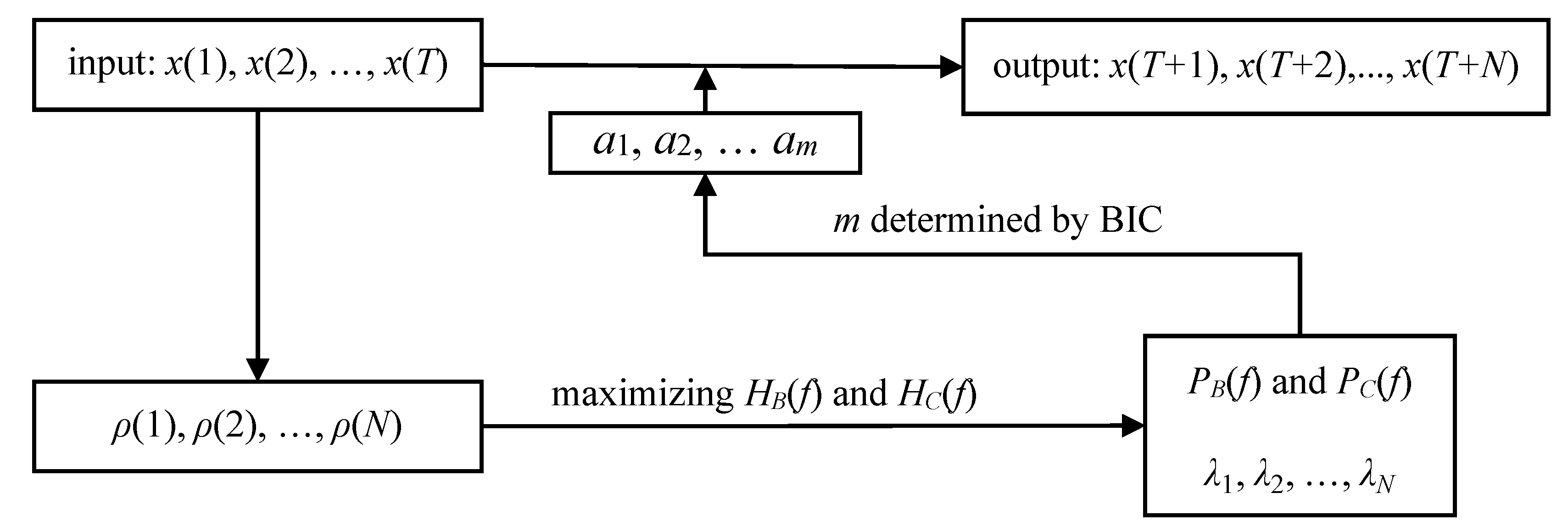
Figure 2.
The location of selected stations.
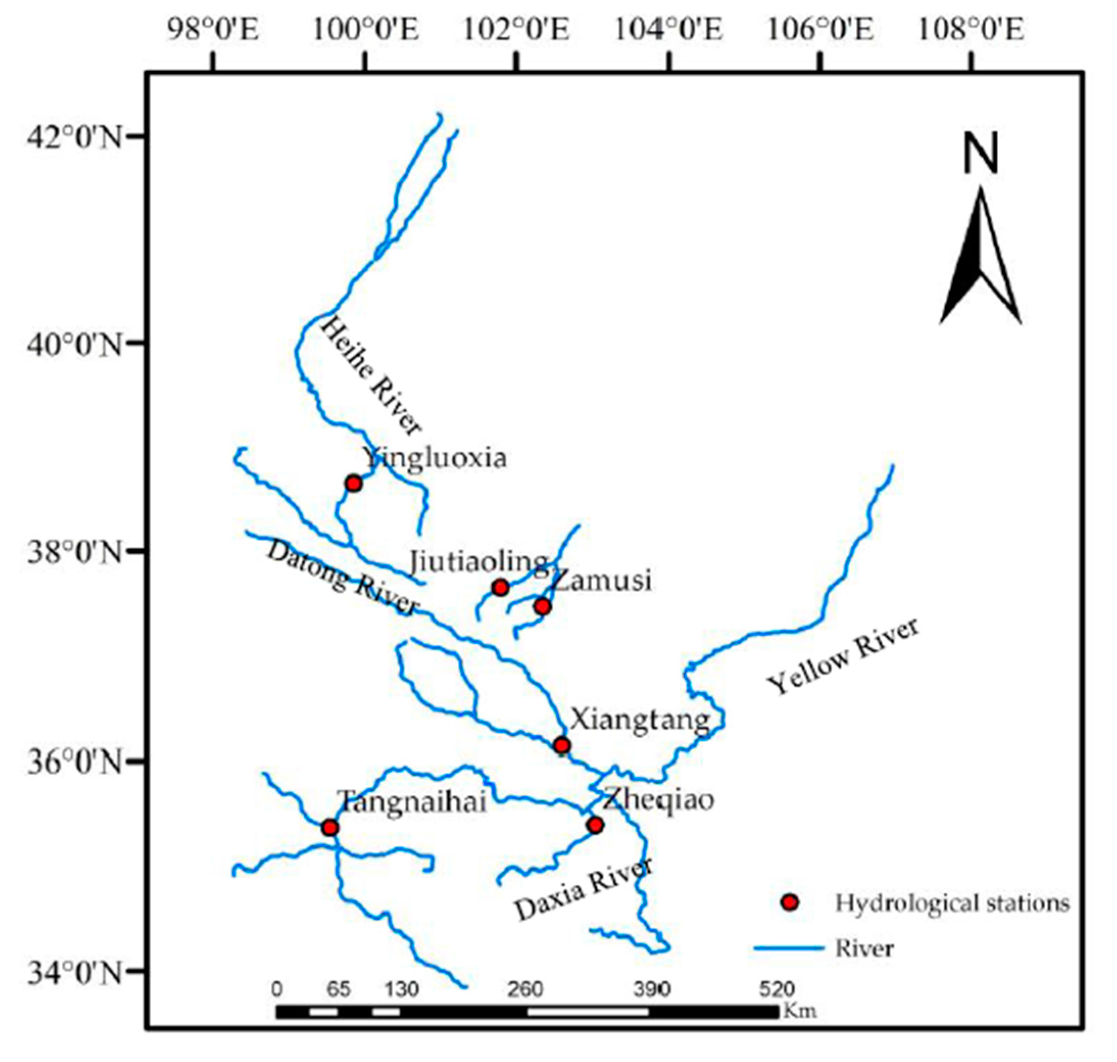
Figure 3.
Monthly streamflow for selected stations. (a) Xiangtang station; (b) Yingluoxia station; (c) Zamusi station; (d) Jiutiaoling station; (e) Tangnaihai station; (f) Zheqiao station.
Figure 3.
Monthly streamflow for selected stations. (a) Xiangtang station; (b) Yingluoxia station; (c) Zamusi station; (d) Jiutiaoling station; (e) Tangnaihai station; (f) Zheqiao station.
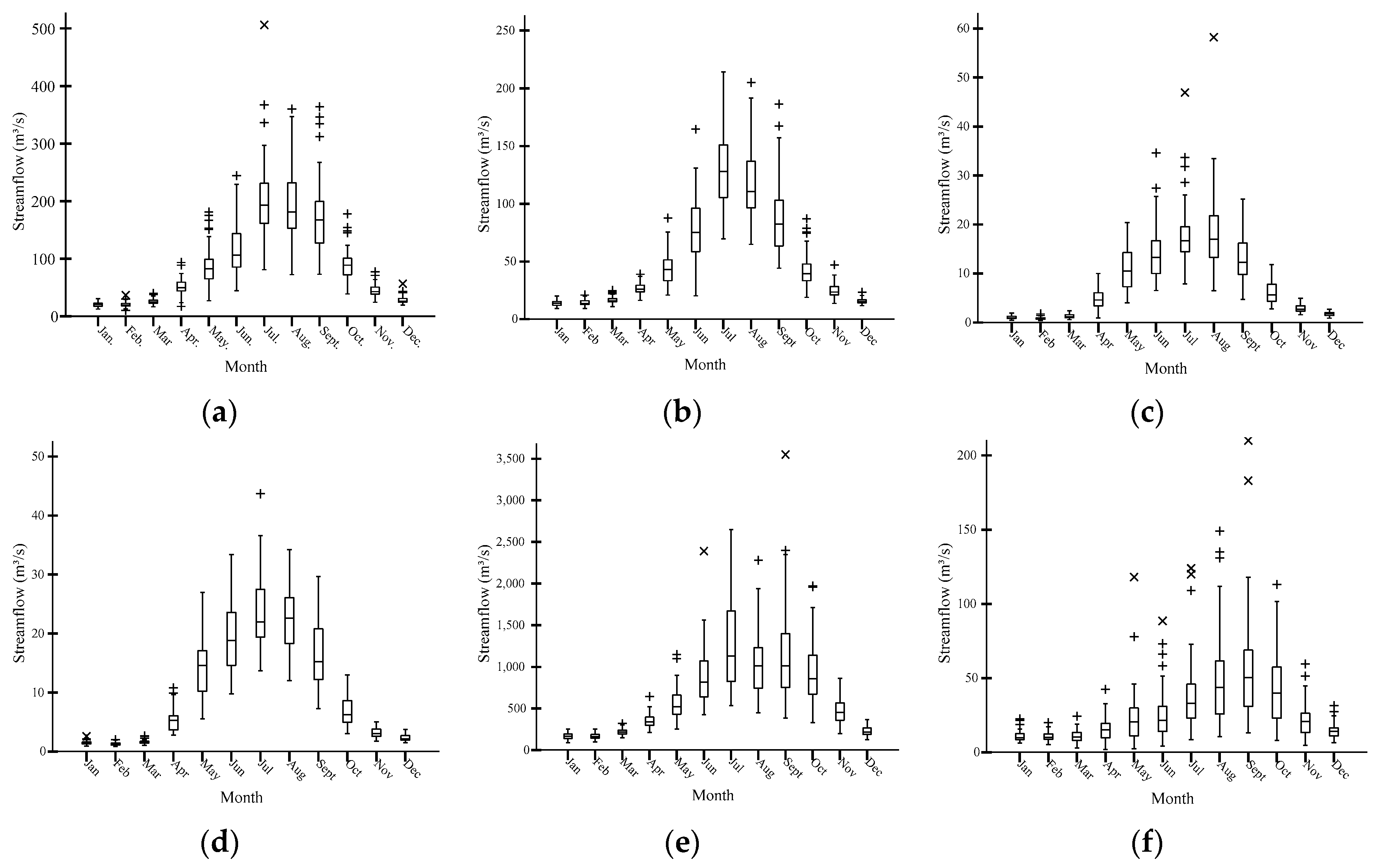
Figure 4.
Streamflow forecasted using entropy spectral analysis of representative stations in training time. (a) Xiangtang station; (b) Yingluoxia station; (c) Zamusi station; (d) Jiutiaoling station; (e) Tangnaihai station; (f) Zheqiao station.
Figure 4.
Streamflow forecasted using entropy spectral analysis of representative stations in training time. (a) Xiangtang station; (b) Yingluoxia station; (c) Zamusi station; (d) Jiutiaoling station; (e) Tangnaihai station; (f) Zheqiao station.

Figure 5.
Streamflow forecasted using entropy spectral analysis of representative stations in lead time. (a) Xiangtang station; (b) Yingluoxia station; (c) Zamusi station; (d) Jiutiaoling station; (e) Tangnaihai station; (f) Zheqiao station.
Figure 5.
Streamflow forecasted using entropy spectral analysis of representative stations in lead time. (a) Xiangtang station; (b) Yingluoxia station; (c) Zamusi station; (d) Jiutiaoling station; (e) Tangnaihai station; (f) Zheqiao station.

Figure 6.
Forecasted values of Burg entropy spectral analysis (BESA) related to observed values in the lead time. (a) Xiangtang station; (b) Yingluoxia station; (c) Zamusi station; (d) Jiutiaoling station; (e) Tangnaihai station; (f) Zheqiao station.
Figure 6.
Forecasted values of Burg entropy spectral analysis (BESA) related to observed values in the lead time. (a) Xiangtang station; (b) Yingluoxia station; (c) Zamusi station; (d) Jiutiaoling station; (e) Tangnaihai station; (f) Zheqiao station.

Figure 7.
Forecasted values of configurational entropy spectral analysis (CESA) related to observed values in the lead time. (a) Xiangtang station; (b) Yingluoxia station; (c) Zamusi station; (d) Jiutiaoling station; (e) Tangnaihai station; (f) Zheqiao station.
Figure 7.
Forecasted values of configurational entropy spectral analysis (CESA) related to observed values in the lead time. (a) Xiangtang station; (b) Yingluoxia station; (c) Zamusi station; (d) Jiutiaoling station; (e) Tangnaihai station; (f) Zheqiao station.

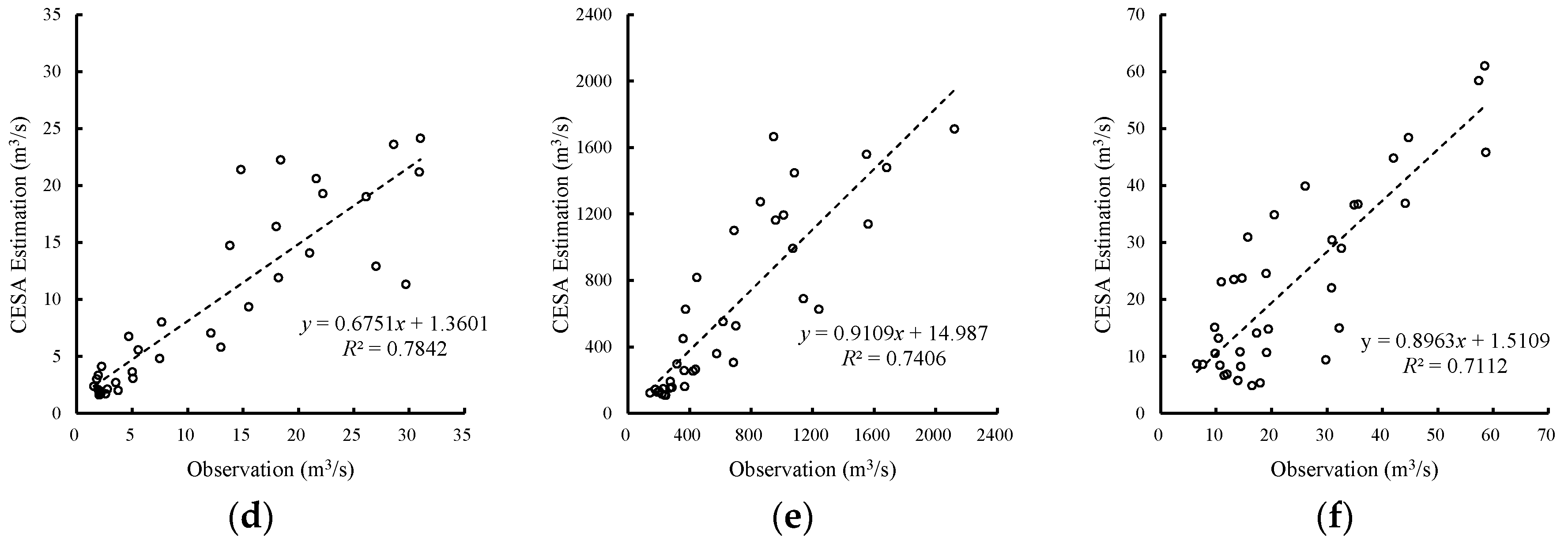
Figure 8.
Autocorrelation plot of representative stations. (a) Xiangtang station; (b) Yingluoxia station; (c) Zamusi station; (d) Jiutiaoling station; (e) Tangnaihai station; (f) Zheqiao station.
Figure 8.
Autocorrelation plot of representative stations. (a) Xiangtang station; (b) Yingluoxia station; (c) Zamusi station; (d) Jiutiaoling station; (e) Tangnaihai station; (f) Zheqiao station.


Table 1.
Basic information of steamflow data for selected stations.
| No. | Station | Longitude | Latitude | River | Basin Area (km2) | Catchment Area (km2) | Record Length | Average (m3/s) | Peak (m3/s) |
|---|---|---|---|---|---|---|---|---|---|
| 1 | Xiangtang | 102°51′E | 36°22′N | Datong | 15133 | 15,126 | 1950–2016 | 88 | 506 |
| 2 | Yingluoxia | 100°11′E | 38°48′N | Heihe | 130,000 | 10,009 | 1954–2012 | 51 | 214 |
| 3 | Zamusi | 102°34′E | 37°42′N | Zamu | 851 | 851 | 1952–2010 | 8 | 58.2 |
| 4 | Jiutiaoling | 102°03′E | 37°52′N | Xiying | 1120 | 1077 | 1972–2010 | 10 | 43.7 |
| 5 | Tangnaihai | 100°09′E | 35°30′N | Yellow | 752,443 | 121,972 | 1956–2016 | 633 | 3550 |
| 6 | Zheqiao | 103°16′E | 35°38′N | Daxia | 7154 | 6843 | 1963–2016 | 27 | 210 |
Table 2.
Results of forecasting at representative stations by two entropy methods.
| Station | Model | Model Order | Training Time (2003–2007) | Lead Time (2008–2010) | ||||||
|---|---|---|---|---|---|---|---|---|---|---|
| RE | RMSE | R2 | NSE | RE | RMSE | R2 | NSE | |||
| xiangtang | BESA | 16 | 0.169 | 19.4 | 0.953 | 0.904 | 0.376 | 27.3 | 0.913 | 0.773 |
| CESA | 11 | 0.231 | 24.5 | 0.920 | 0.840 | 0.405 | 28.1 | 0.890 | 0.760 | |
| yingluoxia | BESA | 8 | 0.202 | 17.3 | 0.915 | 0.834 | 0.235 | 21.2 | 0.912 | 0.798 |
| CESA | 10 | 0.267 | 22.8 | 0.874 | 0.708 | 0.185 | 21.1 | 0.917 | 0.801 | |
| zamusi | BESA | 14 | 0.207 | 2.7 | 0.913 | 0.832 | 0.268 | 2.5 | 0.925 | 0.838 |
| CESA | 12 | 0.316 | 3.7 | 0.864 | 0.690 | 0.382 | 3.5 | 0.840 | 0.684 | |
| jiutiaoling | BESA | 11 | 0.229 | 4.5 | 0.920 | 0.768 | 0.245 | 4.9 | 0.915 | 0.755 |
| CESA | 13 | 0.346 | 5.1 | 0.868 | 0.697 | 0.318 | 5.4 | 0.886 | 0.707 | |
| tangnaihai | BESA | 13 | 0.312 | 303.3 | 0.750 | 0.548 | 0.295 | 354.8 | 0.759 | 0.482 |
| CESA | 8 | 0.335 | 340.3 | 0.805 | 0.447 | 0.360 | 273.0 | 0.861 | 0.693 | |
| zheqiao | BESA | 15 | 0.362 | 19.0 | 0.621 | 0.255 | 0.291 | 9.1 | 0.876 | 0.618 |
| CESA | 8 | 0.466 | 17.8 | 0.640 | 0.365 | 0.369 | 8.6 | 0.843 | 0.659 | |
Table 3.
Comparison of the performance metrics by four models.
| Station | BESA | CESA | AR | SAR | ||||
|---|---|---|---|---|---|---|---|---|
| NSE of TT | NSE of LT | NSE of TT | NSE of LT | NSE of TT | NSE of LT | NSE of TT | NSE of LT | |
| xiangtang | 0.904 | 0.773 | 0.840 | 0.760 | 0.686 | 0.666 | 0.564 | 0.631 |
| yingluoxia | 0.834 | 0.798 | 0.708 | 0.801 | 0.612 | 0.755 | 0.429 | 0.624 |
| zamusi | 0.832 | 0.838 | 0.690 | 0.684 | 0.644 | 0.524 | 0.479 | 0.540 |
| jiutiaoling | 0.768 | 0.755 | 0.697 | 0.707 | 0.585 | 0.511 | 0.456 | 0.466 |
| tangnaihai | 0.548 | 0.482 | 0.447 | 0.693 | 0.495 | 0.34 | 0.403 | 0.373 |
| zheqiao | 0.255 | 0.618 | 0.365 | 0.659 | 0.485 | 0.144 | 0.364 | 0.728 |
Notes: TT represents training time and LT represents lead time. AR: autoregressive; SAR: seasonal autoregressive.
© 2017 by the authors. Licensee MDPI, Basel, Switzerland. This article is an open access article distributed under the terms and conditions of the Creative Commons Attribution (CC BY) license (http://creativecommons.org/licenses/by/4.0/).
Share and Cite
MDPI and ACS Style
Zhou, Z.; Ju, J.; Su, X.; Singh, V.P.; Zhang, G. Comparison of Two Entropy Spectral Analysis Methods for Streamflow Forecasting in Northwest China. Entropy 2017, 19, 597. https://doi.org/10.3390/e19110597
AMA Style
Zhou Z, Ju J, Su X, Singh VP, Zhang G. Comparison of Two Entropy Spectral Analysis Methods for Streamflow Forecasting in Northwest China. Entropy. 2017; 19(11):597. https://doi.org/10.3390/e19110597
Chicago/Turabian StyleZhou, Zhenghong, Juanli Ju, Xiaoling Su, Vijay P. Singh, and Gengxi Zhang. 2017. "Comparison of Two Entropy Spectral Analysis Methods for Streamflow Forecasting in Northwest China" Entropy 19, no. 11: 597. https://doi.org/10.3390/e19110597
Note that from the first issue of 2016, this journal uses article numbers instead of page numbers. See further details here.