Understanding the Fractal Dimensions of Urban Forms through Spatial Entropy


1
Department of Geography, College of Urban and Environmental Sciences, Peking University, Beijing 100871, China
2
Department of Urban Planning and Management, School of Public Administration and Policy, Renmin University of China, Beijing 100872, China
*
Author to whom correspondence should be addressed.
Entropy 2017, 19(11), 600; https://doi.org/10.3390/e19110600
Submission received: 17 September 2017
/
Revised: 29 October 2017
/
Accepted: 6 November 2017
/
Published: 9 November 2017
(This article belongs to the Special Issue Geometry in Thermodynamics II)
Abstract
:The spatial patterns and processes of cities can be described with various entropy functions. However, spatial entropy always depends on the scale of measurement, and it is difficult to find a characteristic value for it. In contrast, fractal parameters can be employed to characterize scale-free phenomena and reflect the local features of random multi-scaling structure. This paper is devoted to exploring the similarities and differences between spatial entropy and fractal dimension in urban description. Drawing an analogy between cities and growing fractals, we illustrate the definitions of fractal dimension based on different entropy concepts. Three representative fractal dimensions in the multifractal dimension set, capacity dimension, information dimension, and correlation dimension, are utilized to make empirical analyses of the urban form of two Chinese cities, Beijing and Hangzhou. The results show that the entropy values vary with the measurement scale, but the fractal dimension value is stable is method and study area are fixed; if the linear size of boxes is small enough (e.g., <1/25), the linear correlation between entropy and fractal dimension is significant (based on the confidence level of 99%). Further empirical analysis indicates that fractal dimension is close to the characteristic values of spatial entropy. This suggests that the physical meaning of fractal dimension can be interpreted by the ideas from entropy and scaling and the conclusion is revealing for future spatial analysis of cities.
1. Introduction
No one is considered scientifically literate today who does not know what a Gaussian distribution is or the meaning and scope of the concept of entropy. It is possible to believe that no one will be considered scientifically literate tomorrow who is not equally familiar with fractals.—Attributed to John A. Wheeler (1983)
Entropy has been playing an important role for a long time in both spatial measurements and mathematical modeling of urban studies. When mathematical methods were introduced into geography from 1950s to 1970s, the ideas from system theory were also introduced into geographical research. The mathematical methods lead to computational geography and further geo-computation (GC) science, and the system methods result to geographical informatics and then geographical information science (GISc). Along with system thinking, the concepts of entropy entered geographical analysis [1], and the notion of spatial entropy came into being [2]. On the one hand, entropy as a measurement can be used to make spatial analysis for urban and regional systems [2,3,4,5]; on the other, the entropy maximizing method (EMM) can be employed to constitute postulates and make models for human geography [6,7,8,9,10,11,12,13]. Unfortunately, the empirical values of spatial entropy often depend on the scale of measurement, and it is difficult to find determinate results for given study area in many cases. The uncertainty of spatial entropy seems to be associated with the well-known modifiable areal unit problem (MAUP) [14,15,16,17]. The essence of geographical uncertainty such as MAUP rests with the scaling invariance in geographical space. In short, the spatial measures of a Euclidean object is independent of linear scales (scale-free), but urban measurements rely heavily on the corresponding linear sizes of areal units (scale-dependent), and as a result, we cannot obtain determinate values for urban area and density [18,19].
One of the most efficient approaches to addressing scale-free problems is fractal geometry. Many outstanding issues are now can be resolved due to the advent of the fractal theory [20]. Fractal geometry is a powerful tool in spatial analysis, showing a new way of looking at urban and regional systems [21,22,23]. In a sense, fractal dimension is inherently associated with entropy. On the one hand, the generalized fractal dimension is based on Renyi’s entropy [24]; on the other, it was demonstrated that Hausdorff’s dimension is mathematically equivalent to Shannon’s entropy [25]. In urban studies, both entropy and fractal dimension can be adopted to measure the space filling extent and spatial complexity of urban growth, and thus can be employed to characterize the compactness of urban form or regularity of urban boundaries. If the entropy value is not determinate due to scale-free distributions, it can be alternatively replaced by fractal dimension. However, in practice, thing is complicated. When and where we should utilize entropy or fractal dimension to make spatial analysis is pending. Preparatory theoretical and empirical studies should be made before clarifying the inner links and essential differences between entropy and fractal dimension.
Geography is a science on spatial difference, and the reflection of difference in human brain yields information. Information can be measured by entropy and fractal dimension. Based on the numerical relations derived from observational data, this paper is devoted to exploring the similarities and differences between entropy and fractal dimension in urban studies. In Section 2, a typical regular growing fractal is taken as an archetype to reveal the connection and distinction between entropy and fractional dimension. The fractal dimension is actually an entropy-based parameter. In Section 3, two Chinese cities, Beijing and Hangzhou, are taken as examples to perform empirical analyses. The linear correlation between entropy and fractal dimension is displayed for given scale and study area. The results will show that the entropy values rely heavily on spatial scale of measurement, but fractal dimension values are scale-free parameters. In Section 4, the main points of this work are outlined, and the shortcomings of the case analyses are stated. Finally, the discussion is concluded by summarizing the principal viewpoints of this study.
2. Theoretical Models
2.1. The Relation of Fractal Dimension to Entropy
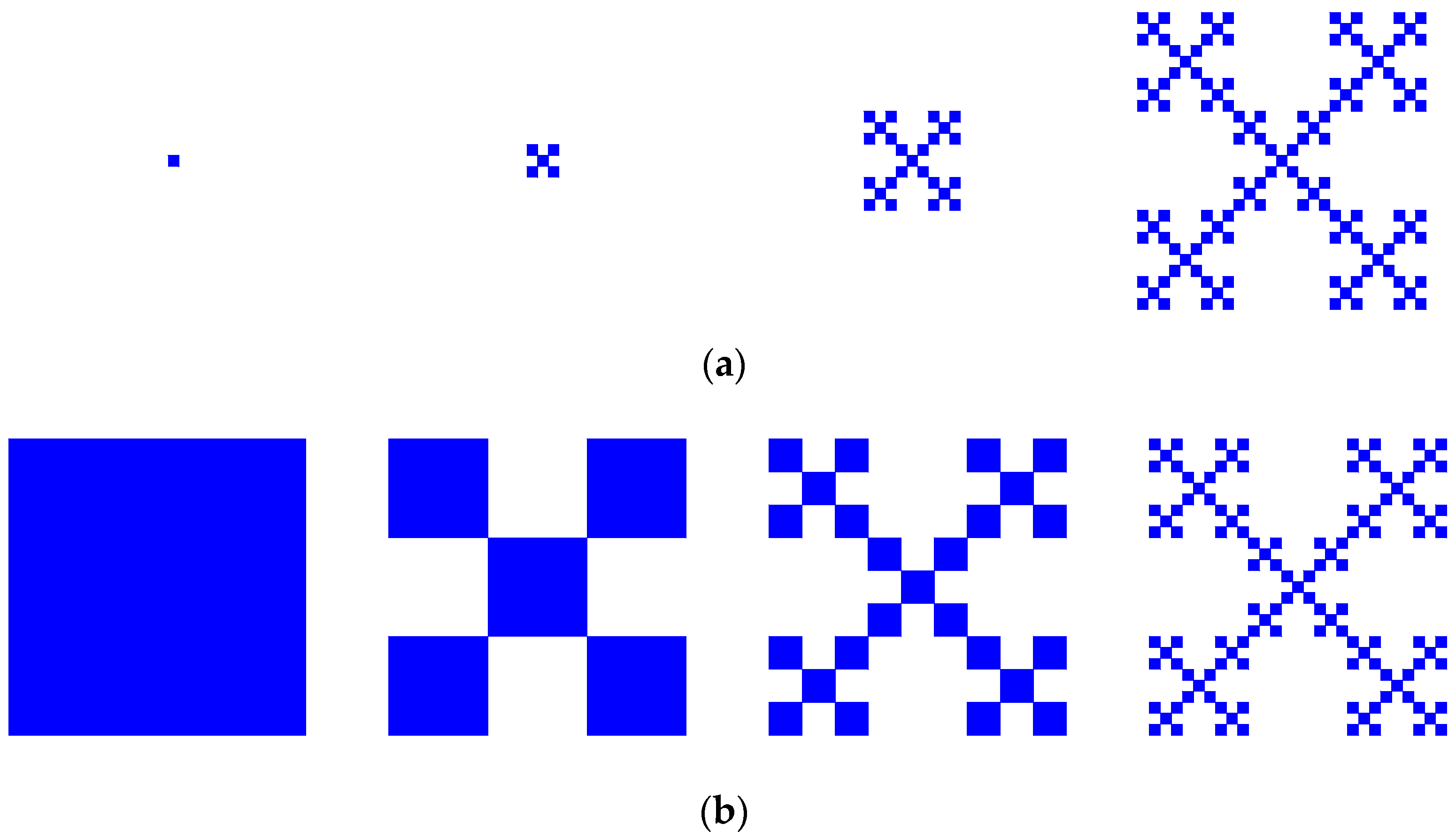
Fractal dimension is a measurement of space-filling extent. For urban growth and form, fractal dimension, including box dimension and radial dimension, can act as two indices. One is the index of uniformity for spatial distribution, and the other is the index of space occupancy indicating land use intensity and built-up extent. What is more, the box dimension is associated with spatial entropy [26], and the radial dimension associated with the coefficient of spatial autocorrelation [27]. High fractal dimension suggests low spatial difference and strong spatial correlation between urban parts. For simplicity, let’s see a typical growing fractal, which bear an analogy with urban form and growth (Figure 1). This fractal was proposed by Jullien and Botet [28] and became well known due to the work of Vicsek [29], and it is also termed Vicsek’s figure or box fractal. Geographers employed it to symbolize fractal growth of cities [23,30,31,32,33]. Starting from an initiator, a point or a square, we can generate the growing fractal by infinitely cumulating space filling or recursive subdivision of space. It is convenient to compute the spatial entropy and fractal dimension of this kind of fractal objects.
The precondition of an index as an effective measurement is that it bears a determinate value and clear limits. Or else, facing uncertain calculation results, researchers will feel puzzled. However, for the systems without characteristic scale such as fractal cities, we cannot find a determinate entropy value to describe them. In order to compute the spatial entropy, we can use a set of proper grids, i.e., nothing more, nothing less, to cover a figure. This approach is similar to the box-counting method in fractal studies. A grid consists of a number of squares, which bear an analogy with the boxes for fractal dimension measurement. Sometimes, different types of grid lead to different evaluations. Let’s take the well-known box fractal as an example to illustrate the scale dependence of entropy value (Figure 1). If we use a grid comprising a square as a “box” to encompass the fractal object, the “box” just covers the fractal, nothing more, and nothing less. The size of the box is just the measure area of the fractal. In mathematics and fractal geometry, the so-called measure area is the area of the smallest circumscribed rectangle of a geometric shape. Thus, the macro state number and probability are N = P = 1, the spatial entropy is H = −Pln(P) = ln(N) = 0. If the square is averaged into nine parts, than we have a grid comprising nine small squares formed by crossed lines. This time, there are five nonempty “boxes”. The macro state number is N = 5, the spatial distribution probability is P = 1/N = 1/5, and the spatial entropy is H = −∑Pln(P) = ln(N) = ln(5) = 1.609 nat. Dividing the nine small squares into 81 much smaller squares of the same size yields 25 nonempty “boxes”. Thus the spatial entropy is H = 2 × ln(5) = 3.219 nat, and so on. In short, for the monofractal object, the information entropy equals the corresponding macro state entropy. For the fractal copies with a linear size of ε = 1/3m−1, we have:
in which m represents the step numbering of fractal generation (m = 1, 2, 3, …), and m − 1 denotes the exponent of scale. This suggests that the spatial entropy H(ε) values depend on the scale of measurement ε. However, if we examine the relationship between the scale series ε = 1, 1/3, 1/9, …, 1/3m−1 and nonempty box number series N(ε) = 1, 5, 25, …, 5m−1, we will find a power function N(ε) = ε−D, where the scaling exponent D = ln(5)/ln(3) = 1.465. This exponent value is foreign to the scale 3m−1. The scaling exponent is just the fractal dimension of the box fractal. The entropy values are indeterminate, but the fractal dimension value is one and only (Table 1).
As indicated above, for a simple fractal object, the macro state entropy based on fractal copy number is equal to the information entropy based on growth probability. The fractal dimension can be defined by the ratio of the state entropy to the logarithm of the linear size of fractal copies. Given a linear size of fractal copies ε and the number of fractal copies N(ε), Shannon’s information entropy is:
where N(ε) denotes the number of fractal copies with linear size ε, Pi(ε) refers to the probability of growth of the i-th fractal copy. For the simple regular fractals, the growth probabilities of different fractal copies are equal to one another, i.e., Pi(ε) = 1/N(ε). Therefore, the macro state entropy equals the information entropy, that is:
in which S indicates the state entropy of urban form. The capacity dimension of fractals is defined based on the state entropy such as:
where D0 denotes the capacity dimension. However, for a complex multifractal object, the information entropy is less than the macro state entropy. Based on the information entropy, the information dimension is defined by:
where D1 refers to the information dimension.
The state entropy and information entropy can be unified formally. Generalizing varied entropy functions, Renyi [34] proposed a universal formula to define entropy, which can be expressed as:
where q denotes the order of moments. If q = 0, M0 = S represents macro state entropy; If q = 1, M1 = H represents Shannon information entropy; if q = 2, M2 denotes correlation entropy. As a spatial measure, Renyi entropy has been successfully applied to the studies on regional land use and urban sprawl [35,36], and the results are revealing for geographers. In fact, different types of fractal dimension can be integrated into an expression by Renyi’s entropy. Based on Equation (5), the generalized correlation dimension can be defined in the following form [24,37,38]:
where Dq is the generalized dimension of order q. If q = 0, Dq = D0 refers to capacity dimension, if q = 1, Dq = D1 refers to information dimension, and if q = 2, Dq = D2 refers to correlation dimension [39]. In theory, q ∈ (−∞, +∞). Thus we get a multifractal spectrum based on q. For the monofractal phenomena, D0 = D1 = D2, but for the multifractal systems, D0 > D1 > D2.
2.2. Entropy and Fractal Dimension Indicating Geo-Spatial Development
Fractal theory suggests a new way of mathematical modeling, especially in geographical analysis. In future science, culture, and education, fractal concepts will play an important role and will become as common as entropy and maps [40,41]. In fact, entropy can be associated with fractal dimension by both mathematical forms and physical meaning. For a given linear scale ε, the fractal dimension is equivalent to the corresponding entropy. The generic conclusion was drawn by Ryabko [25], who argued that the Shannon’s entropy is equivalent in mathematics to the Hausdorff dimension. Both entropy and fractal dimension can be employed to describe urban form and growth, reflecting space filling extent and spatial uniformity. Fractal dimension changes can reflect spatial concentration and diffusion. As mentioned above, we have two typical approaches to constructing the deterministic fractals. One is to use an iteration procedure, and the other is by subsequent divisions of the original square [29]. The former process bears an analogy with urban growth, while the latter process has an analogy to regional agglomeration (Figure 1). The same goal can be reached by different routes. That is, the final results are the same with each other, and the fractal dimension is D = ln(5)/ln(3) = 1.465. Now, let’s examine the processes of a fractal development rather than its final result. For the fractal process in Figure 1a, the initiator is a point with dimension D = 0, corresponding to the information entropy H = 0, but the final dimension is D = 1.465, corresponding to the information entropy H = 1.609. The dimension value and information entropy go up (from 0 to 1.465, 0 to 1.609). For the fractal process in Figure 1b, the initiator is a square with dimension D = 2, corresponding to the information entropy H = 2.197, but the final dimension is D = 1.465. The dimension value and information entropy go down (from 2 to 1.465, 2.197 to 1.609). Figure 1a suggests a process of spatial spread, while Figure 1b implies a process of spatial concentration. In order to reveal the numerical relation between spatial entropy and fractal dimension, we can investigate real urban systems which are more complicated than the regular fractal shown above.
3. Materials and Methods
3.1. Study Area, Data, and Approaches
The spatial entropy and fractal parameters can be employed to make empirical analyses of the urban form and growth. One example is Beijing, the national capital of China, and the other example is Hangzhou, the provincial capital of Zhejiang, China. The datasets of Beijing city are involved with five years, that is, 1988, 1992, 1999, 2006, and 2009 (Figure 2). The original data are extracted from the remote sensing images, including three Landsat TM images and two Landsat ETM+ images. The ground resolution of these images is 30 m [42]. The functional box-counting method can be used to measure the spatial entropy and fractal dimension (Figure 3). This method was originally adopted by Lovejoy et al. [43] to analyze radar rain data, and Chen [26] improved this method in urban studies by replacing the largest box (the first level box) with arbitrary area with the largest box with a measure area of an urban system. In fact, the functional box-counting method can be termed Rectangle Space Subdivision (RSS) method [42,44]. The geometrical basis of RSS is the recursive subdivision of space and the cascade structure of hierarchies [30,45]. Its mathematical basis is the logical relationship between the exponential laws based on translational symmetry and the power laws based on dilation symmetry [9]. This method can better reflect the cascade structure of a fractal city, and thus better estimate its fractal dimension.
3.2. Results and Findings Based on Fixed Box Method
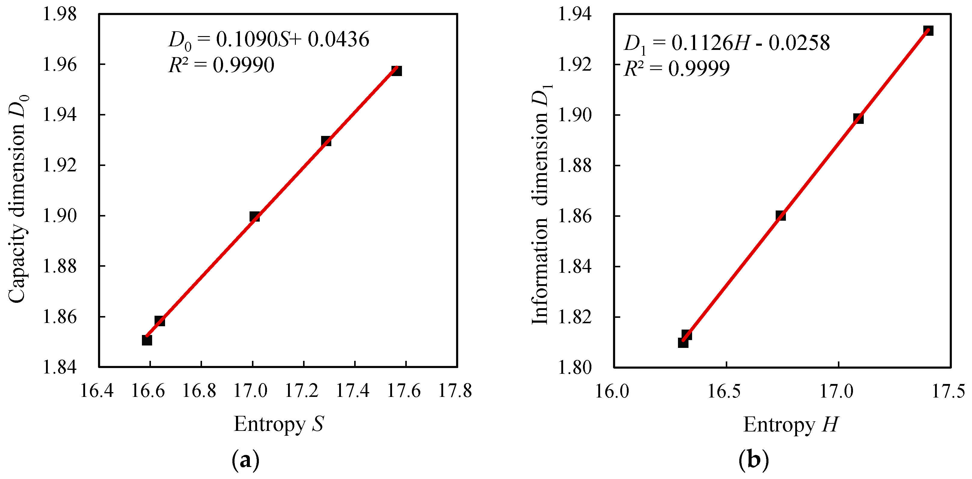
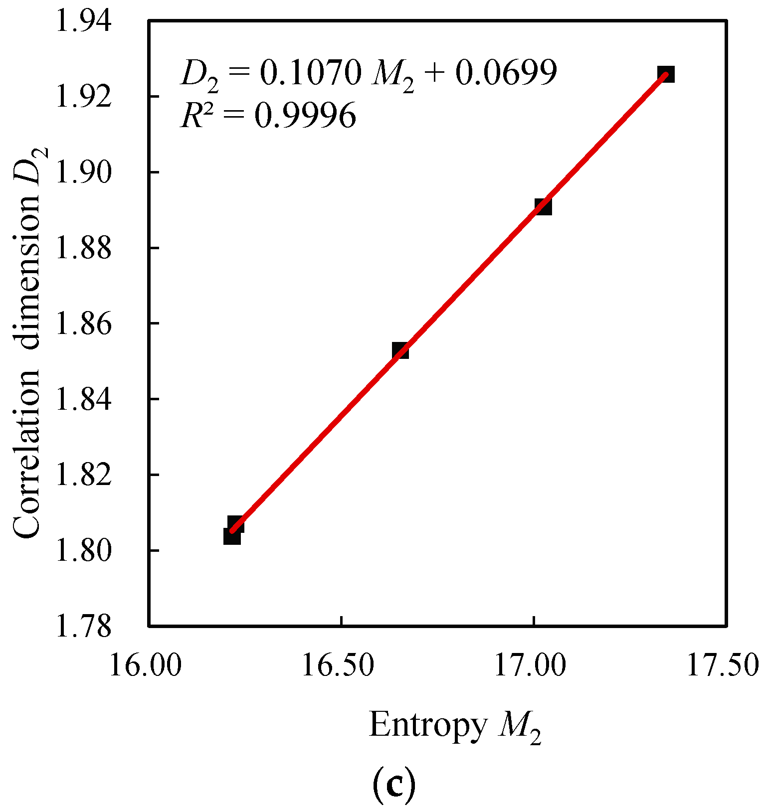
Applying the functional box method above-illustrated to Beijing metropolitan area yields the datasets of the spatial distribution of urban land use in five years. Two types of box counting can be applied to fractal dimension estimation of cities [31,42]: one is to fix the largest box [46], and the other is to unfix the largest box [44]. In the former way, the size and shape of the first level box do no change for different years; in the latter way, the size and shape of the largest box change with urban growth in different years. For comparability, the box size is fixed for the five years. The area of the largest box equals the measure area of the metropolis in 2009. Using the datasets, we can calculate state entropy, information entropy, and Renyi entropy (Table 2). The relationships between the logarithms of the linear size of box (scale) and the entropy values (measurements) take on a linear trend (Figure 4). The slopes of the trend lines give the capacity dimension D0, information dimension D1, and correlation dimension D2. As indicated above, D0 is based on macro state entropy (Boltzmann entropy), D1 is based on information entropy (Shannon entropy), and D2 is based on generalized entropy (Renyi entropy). The standard errors of all the fractal dimension values are less than 0.04. According to Benguigui et al. [46], whose fractal discriminant criterion is standard error σ < 0.04, the fractal structure of Beijing’s urban form is significant because the errors of fractal dimension values are less than 0.1 (Table 3).
The calculation results of entropy and fractal dimension reflect the following characteristics. First, the entropy and fractal dimension increased monotonically from 1988 to 2009. This suggests that the city had been growing and its urban space was constantly filled. Second, entropy and fractal dimension rose in parallel in these years. The entropy values and fractal dimension curves can be modeled by quadratic logistic function, which indicates the replacement dynamics of fast growth. Third, the capacity value of the fractal dimension in the quadratic logistic models are Dmax = 2. This suggests that the urban space of Beijing’s metropolitan area will be over filled. Normally, the capacity parameter Dmax < 2. Otherwise, the city will have not enough vacant land and open space in future. The empirical results support the above-shown theoretical inference based on regular fractals. For the urban agglomeration of Beijing, the spatial entropy values depend on the scale of measurements. When the linear size of boxes becomes smaller and smaller, the entropy values become larger and larger. No characteristic entropy value can be found for spatial description. However, there is a determinate relation between the linear sizes of boxes and the corresponding entropy values. By this relation, a number of entropy values can be transformed into a fractal dimension value. In other words, we cannot find a characteristic scale for entropy measurement, but we can use fractal dimension as an alternative characteristic parameter to reflect urban spatial structure.
Now, let’s examine the correlation relationships between three types of entropy and the corresponding fractal dimensions. As indicated above, for given moment orders (q), based on different linear sizes of boxes (ε), we have different entropy values, but the corresponding fractal dimension value does not depend on the linear sizes. Using the datasets of entropy and fractal dimension values, we can calculate the square of correlation coefficients (R squared). The squared R is known as goodness of fit or determination coefficient in linear regression analysis (Table 4). The results show three characters. First, the smaller the linear sizes of boxes, the higher the squared correlation coefficient values; second, the closer to q = 1 the moment order, the higher the squared correlation coefficient values tend to be; third, there seems to be a limit for the smallest linear size of boxes (Figure 5). The relation between entropy (Mq) and fractal dimension (Dq) can be expressed as Dq = a + bMq, where a and b are constants. This suggests that the fractal dimension of cities includes the meaning of spatial entropy. If the linear size of spatial measurement is small enough, the entropy and fractal dimension can be replaced with one another in theory, and supplement each other in practice.
3.3. Observational Evidences and Findings Based on Unfixed Box Method
More empirical evidence can be found to attest the numerical relationships between spatial entropy and fractal dimension. The city of Hangzhou is another typical example. The spatial patterns of Hangzhou’s urban land use bear fractal structure, and can be characterized with fractal dimension (Figure 6). Using the functional box-counting method, Feng and Chen [44] once calculated the capacity dimension of Hangzhou’s urban form in four different years (1949, 1959, 1980, and 1996). Different from the case of Beijing city, the variable boxes were employed to make spatial measurement for suiting city sizes in different years. Unfortunately, owing to the limitations of data, information dimension and correlation dimension cannot be calculated for Hangzhou’s urban form.
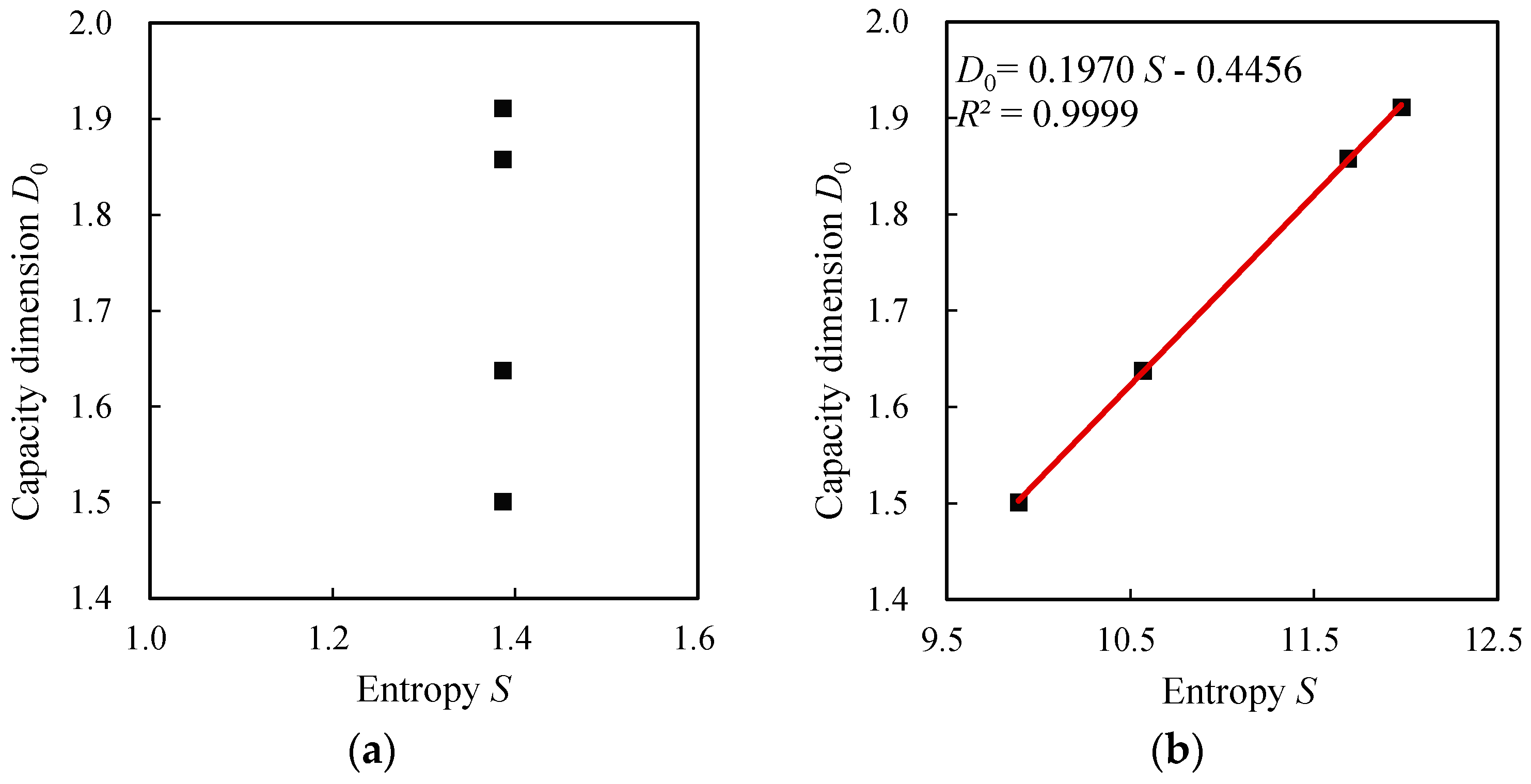
The analytical process is similar to that is made for Beijing city. The difference lies in that the largest box is adjusted to suit the city size in different years. Based on the published datasets by Feng and Chen [44], the macro state entropy can be computed and the coefficient of correlation between state entropy and capacity dimension values can be worked out (Table 5). The conclusions from the calculation results of Hangzhou are similar to those of Beijing. The difference lie the sigmoid curves of entropy and fractal dimension increase. The data can be fitted by the common logistic function, which represents the spatial replacement dynamics of natural growth [31]. The capacity parameter of the logistic model of the fractal dimension curve is about Dmax = 1.95 < 2. This implies that Hangzhou’s urban space will not be completely filled in future. Positive analysis for urban evolution is not the main topic of this work. According to the results, when the linear sizes of boxes become smaller and smaller, the linear relationships between entropy and fractal dimension become clearer and clearer. For the large size of boxes, the regularity does not appear; if the box sizes become small enough, the linear fit of fractal dimension to entropy is close to perfection (Figure 7).
In statistics, if R2 = 1, the regression effect is termed perfect fit. The relation between entropy (S) and fractal dimension (D0) can be written as D0 = a + bS, where a and b are parameters. This case lends further support the inference that there is potential equivalence of fractal dimension to entropy under certain condition, for example, the box-counting method is employ to make spatial measurement. The smaller the boxes, the closer the entropy value is to the fractal dimension. However, the urban density of population distribution in Hangzhou can be described with spatial entropy rather than fractal dimension. Urban population density follows Clark’s law [47], which suggests a characteristic scale by radius length [48]. Clark’s law can be expressed as a negative exponential function:
where ρ(r) denotes the population density at the distance r from the center of city (r = 0). As for the parameters, ρ0 refers to the urban central density ρ(0), and r0 to the characteristic radius of the population distribution [3,48]. The negative exponent distribution differs from the inverse power-law distribution. The former bears characteristic scale r0, while the latter possesses no characteristic scale. For the distribution with characteristic scale, we cannot calculate fractal dimension, but we can compute the spatial entropy using the urban density data. If we want to describe the urban population density using fractal parameters, we must generalize the fractal measure to develop new multifractal indicators. However, by means of the example of urban population distribution, we can illustrate the concept of eigen entropy, which is approximately equal to the corresponding fractal dimension value. The population density data of Hangzhou city based on four years of census (1964, 1980, 1990, and 2000) was processed by Feng [49]. Using these data sets, we can evaluate the spatial information entropy of urban density distribution (Table 6). The characteristic parameter is the average radius of population distribution (r0), which can be estimated with Equation (7). This radius indicates that the central density is associated with the maximum entropy [8].
In fact, urban form has no characteristic scale, but spatial entropy bear characteristic values. In other words, despite that spatial entropy values depend on measurement scales, but entropy itself has a characteristic scale. It can be demonstrated that the characteristic value is just the corresponding fractal dimension. This can be understood by analogy with Clark’s law above mentioned. In the formulae of fractal dimensions, entropy is a logarithmic function of spatial scales. The inverse function is just exponential function, which bears an analogy with Equation (7). In fact, from Equation (6) it follows:
in which a refers to proportionality coefficient, and b = 1/Dq represents the decay parameter. Equation (8) is identical in form to Equation (7). Comparing Equation (8) with Equation (7) suggests that fractal dimension Dq is just the characteristic value of general entropy Mq relative to the linear scale ε. This judgment can be verified by the observational data of Beijing city. Taking logarithm of Equation (8) gives a linear equation such as ln(ε) = ln(a) + b × Mq. Suppose that Mq serves for an independent variable and ln(ε) acts as an dependent variable. The least squares calculations based on the linear relation and the data sets in Table 2 yield a series of regression coefficients. The reciprocals of these regression coefficients, 1/b, indicate the characteristic scales of spatial entropy H0, H1, and H2 (Table 7). The characteristic values of spatial entropy are very close to the fractal dimension values, which are displayed in Table 3 and Table 7. The similar method can be applied to the datasets of Hangzhou city, and the results are added to the last three lines of Table 5. The reciprocal values of the parameter b is close to the values of the corresponding fractal dimension D0. These results are important for us to understand and interpret fractal dimension by means of spatial entropy.
4. Discussion
In terms of the empirical analysis on fractal cities, the relations and differences between entropy and fractal dimension can be brought to light. In theory, the fractal parameters are defined on the base of entropy functions. The capacity dimension is based on Boltzmann’s macro state entropy, the information dimension is based on Shannon’s information entropy, and the correlation dimension is based on the second order Renyi’s entropy. Both entropy values and fractal dimensions depend on measurement method and the scope (size, central location) of study area (Figure 1 and Table 1). Along with urban growth, all the entropy values increase, and accordingly, fractal dimension values ascend (Table 2 and Table 3). This suggests that both entropy and fractal dimension can be used to describe space filling pattern in the process of city development. Despite the association and similarity, there is significant distinction between spatial entropy and fractal dimension. In urban studies, the entropy values depend on the scale of measurement, and thus we need a set of numbers to characterize a state of urban form. The fractal parameters are based on the concept of scaling, we can use a fractal dimension value to substitute for a number of entropy values. In this sense, fractal theory can provide a simpler approach to spatial analysis of cities. According to the empirical analyses, for a given linear scale ε, the numerical relationship between entropy and fractal dimension can be expressed as a linear function such as Dq = a + bMq, where a and b are two parameters. Where Beijing is concerned, a ≈ 0, b ≈ 1/9; where Hangzhou is concerned, a ≈ 0.1970, b ≈ −0.4456. In fact, the spatial entropy and fractal dimension of Beijing’s urban form were measured with fixed boxes. That is to say, the largest boxes in different years are the same with one another [42]. However, the state entropy and capacity dimension of Hangzhou city were measured by using variable boxes. The size of the largest boxes changed along with city size in each year [44]. This suggests that the methods of spatial measurement impact on the regression coefficients, but the linear relation between entropy and fractal dimension is identifiable.
The value of entropy is related to the state number of a system. The number and distribution of elements in a system determine the entropy value. Thus entropy can reflect the diversity of elements in the system. In literature, entropy is often employed to indicate complexity of systems [50,51,52,53]. In fact, entropy is a criterion rather than an index for complex systems. For the distributions with characteristic scale (characteristic length can be found), e.g., urban population density [47], lognormal distribution of city sizes [54], and link degree distribution of traffic networks [55], entropy is an effective measurement for diversity and complexity degree; however, for the distributions without characteristic scale (characteristic length cannot be found), e.g., urban land use pattern [30], spatial distributions of urban traffic networks [30,56], and Zipf’s distribution of city sizes [9,10,30,54], a single entropy value is not enough to measure complexity. In other words, if a system satisfies normal distribution (at least its probability distributions comply with central limit theorem), it can be effectively measured by entropy. In contrast, if a system satisfies scaling law such as power-law distribution (its probability distribution violates central limit theorem), it cannot be easily measured with entropy. In this case, the entropy should be replaced by fractal dimension. A comparison can be drawn as follows (Table 8).
Another important difference between entropy and fractal dimension lies in global and local analyses. Entropy is mainly used to make global analysis of a complex system, while fractal parameters can be utilized to make both global and local analysis for cities. However, if we want to deeply explore the local features of different parts in a complex system such as urban form, entropy will be limited. In this case, fractal dimensions will play an irreplaceable role. One of basic properties of fractals is entropy conservation in different spatial parts. For a given level of a given fractal object (monofractals, multifractals), the entropy values of different units are the same. Thus, we cannot reveal the local feature by the spatial analysis of entropy. For the monofractal object with one scaling process, the fractal dimension values of different units are equal to one another. However, for the multifractal object with more than one scaling process, different units bear different fractal dimension values, which depend on unit sizes and the probability values of element growth or distribution. Thus, we can adopt multifractal dimensions to characterize the local spatial feature of urban form. A multifractal spectrum based on moment orders can be treated as the result of local scanning and sorting for a complex system [57].
An important question should be discussed here to lessen some possible misunderstanding on fractal dimension estimation of cities from readers. To make or use a mathematical model, we must find an effective algorithm to determine its parameter values. A number of measurement methods are proposed in literature to estimate fractal dimension values [20,24,48]. For urban studies, we have various spatial measurements and fractal parameters [23,30]. Generally speaking, different methods are applied to different directions (different aspects or properties). Sometimes, several different methods can be applied to the same aspect of cities. But unfortunately, different methods often lead to different fractal dimension estimation results, and in many cases, the numerical differences are significant and cannot be ignored. Even for a given method, a fractal dimension value often depends on the size and central location of study area. However, in theory, for a given aspect of a city, we should have a unique fractal dimension value. This is involved with the uncertainty of fractal dimension calculation, which puzzles many fractal scientists. Under this circumstances, how can we understand the advantage of fractal dimension relative to spatial entropy for complex urban phenomena? Our viewpoints are as follows:
- (1)
- The problem of methods. It is hard to find solutions to this kind of problem. In fact, for a random system or based on random variables, it is unlikely to find the true parameter values for a mathematical model. Even for the simplest linear regression model, it is impossible to evaluate the real parameters by empirical analysis. A number of algorithms such as least squares method, maximum likelihood method, major axis, and reduced major axis can be used to estimate the regression coefficients, but different methods result in different parameter values. Scientists then look for comparable parameter values instead of real parameter values.
- (2)
- The problems of fractal objects. The real fractals in geometry are just like the high-dimensional spaces in linear algebra, which can be imagined but can never be observed. All the fractal images we encounter in books and articles represent prefractals rather than real fractals. A real fractal has infinite levels, but a prefractal is a limited hierarchy. The basic property of a random prefractal object is that its scaling is limited. For a given aspect (area or boundary) of a regular monofractal, its fractal dimension value is unique, and the real fractal dimension can be calculated through its prefractal structure. However, for a regular multifractal object, different parts have different local fractal dimension values, and the real fractal dimension values cannot be computed by applying a geometric method to its prefractal structure. We can compute its actual fractal parameter values by finding the numerical solutions to its multifractal transcendental equation. A city in the real world is actually a complex random multifractal system with prefractal structure. Different sizes of study area bear different global fractal dimensions, and different parts bear different local fractal dimensions. As a result, changing the scope or central location of study area will yield different fractal parameter values. We never know the real fractal dimension value set. Fortunately, as indicated above, we need comparable parameter values rather than real parameter values, and we can utilize multifractal dimension spectrums to make global and local analyses for complex urban morphology.
The shortcomings of this study lie in three aspects. First, the length of the sample paths of entropy and fractal dimension is short. The number of data points of the two Chinese cities, Beijing and Hangzhou, is only four or five. Fortunately, this is not a critical defect. The short sample path leads to the variability instead of bias. In fact, the well-known Moore’s law, which asserts that the number of components in an integrated circuit doubles approximately every two years [58], was put forward by means of five observational data points and four ratios. Subsequently this law is consolidated by a greater number of large datasets [59]. A scientific judgment should be given by confidence statement, which comprises level of confidence and margin of error [60]. The confidence level depends on degree of freedom rather than sample size. The smaller the sample size, the lower the degree of freedom, and the higher the statistical criterion. Second, only the relationships between entropy and box dimension are investigated. As mentioned above, besides box-counting method, the common methods leading to the fractal dimension of urban area include area-radius scaling, density-radius scaling, sandbox method, and wave spectrum scaling. Among these methods, sandbox is a good approach to calculate multifractal parameters [61], and maybe this method can be employed to research entropy and fractal dimension from a new angle of view. Third, multifractal parameters based on Renyi entropy is not discussed in depth. Although three global multifractal parameters are involved in this work, but the problems of deep structure are bypassed owing to the limitation of space. Anyway, this article is just a beginning, and subsequent studies will be reported in succession.
5. Conclusions
The significance of fractal dimension can be puzzled out by resolving the problems of entropy, and both entropy and fractal dimension can be used to make spatial analysis of cities. The two measurements can be associated with one another, but there is significant difference. Clarifying the similarities and differences between them is helpful to the appropriate application of entropy and fractal theories in urban studies. The main conclusions of this paper can be reached as follows. First, the similarities and differences between spatial entropy and fractal dimension of urban form can be partially revealed by box-counting method. Fractal dimension formulae are based on entropy formulate, and both entropy and fractal dimension can be employed to characterize the spatial complexity of cities. The box-counting method provides a convenient approach to examining the relations and differences between entropy and fractal dimension. Using this method, we can find linear relationships between the two measurements. For the simple structure of monofractal cities, the spatial entropy is equivalent in theory to fractal dimension; for the complex structure of multifractal cities, the description based on entropy parameters is complicated, but the fractal dimension description is simple and clear. The advantages of fractal dimension over entropy rest two aspects: fractal dimension values are independent of the scales of measurement, and multifractal parameter can be used to reveal the local feature of urban form. Second, spatial entropy and fractal dimension have different scopes of applications in empirical studies on cities. Due to the similarities above-mentioned, spatial entropy and fractal dimension can be replaced with each other if the ways of measurements are same and the scale effect of spatial measurement is eliminated. However, because of the differences between each other, entropy and fractal dimension have their own directions and scopes of application in urban research. Entropy is suitable for the urban aspects with characteristic scales such as urban population density, while fractal dimension is suitable for the urban aspects without characteristic scales such as urban land use form and traffic network density distributions. Entropy is mainly used to make global analyses and scale analyses for urban structure and function, while fractal dimension can be employed to make global, local, and especially, scaling analyses for the spatial patterns and processes of urban evolution.
Acknowledgments
This research was sponsored by the National Natural Science Foundation of China (Grant No. 41671167). The supports are gratefully acknowledged. Many thanks to the three anonymous reviewers, whose interesting constructive comments are helpful for improving the quality of this paper.
Author Contributions
Yanguang Chen conceived and designed the experiments; Jiejing Wang and Jian Feng performed the experiments; Yanguang Chen analyzed the data; Jiejing Wang and Jian Feng contributed reagents/materials/analysis tools; Yanguang Chen wrote the paper. All authors have read and approved the final manuscript.
Conflicts of Interest
The authors declare no conflict of interest.
References
- Gould, P.R. Pedagogic review: Entropy in urban and regional modelling. Ann. Assoc. Am. Geogr. 1972, 62, 689–700. [Google Scholar] [CrossRef]
- Batty, M. Spatial entropy. Geogr. Anal. 1974, 6, 1–31. [Google Scholar] [CrossRef]
- Batty, M. Entropy in spatial aggregation. Geogr. Anal. 1976, 8, 1–21. [Google Scholar] [CrossRef]
- Chen, Y.-G. The distance-decay function of geographical gravity model: Power law or exponential law? Chaos Solitons Fractals 2015, 77, 174–189. [Google Scholar] [CrossRef]
- Wilson, A.G. Complex Spatial Systems: The Modelling Foundations of Urban and Regional Analysis; Pearson Education: Singapore, 2000. [Google Scholar]
- Anastassiadis, A. New derivations of the rank-size rule using entropy-maximising methods. Environ. Plan. B Plan. Des. 1986, 13, 319–334. [Google Scholar] [CrossRef]
- Bussiere, R.; Snickers, F. Derivation of the negative exponential model by an entropy maximizing method. Environ. Plan. A 1970, 2, 295–301. [Google Scholar] [CrossRef]
- Chen, Y.-G. A wave-spectrum analysis of urban population density: Entropy, fractal, and spatial localization. Discret. Dyn. Nat. Soc. 2008. [Google Scholar] [CrossRef]
- Chen, Y.-G. The rank-size scaling law and entropy-maximizing principle. Phys. A Stat. Mech. Appl. 2012, 391, 767–778. [Google Scholar] [CrossRef]
- Chen, Y.-G.; Liu, J.-S. Derivations of fractal models of city hierarchies using entropy-maximization principle. Prog. Nat. Sci. 2002, 12, 208–211. [Google Scholar]
- Curry, L. The random spatial economy: An exploration in settlement theory. Ann. Assoc. Am. Geogr. 1964, 54, 138–146. [Google Scholar] [CrossRef]
- Wilson, A.G. Modelling and systems analysis in urban planning. Nature 1968, 220, 963–966. [Google Scholar] [CrossRef] [PubMed]
- Wilson, A.G. Entropy in Urban and Regional Modelling; Pion Press: London, UK, 1970. [Google Scholar]
- Cressie, N.A. Change of support and the modifiable areal unit problem. Geogr. Syst. 1996, 3, 159–180. [Google Scholar]
- Kwan, M.P. The uncertain geographic context problem. Ann. Assoc. Am. Geogr. 2012, 102, 958–968. [Google Scholar] [CrossRef]
- Openshaw, S. The Modifiable Areal Unit Problem; Geo Books: Norwick, UK, 1983. [Google Scholar]
- Unwin, D.J. GIS, spatial analysis and spatial statistics. Prog. Hum. Geogr. 1996, 20, 540–551. [Google Scholar] [CrossRef]
- Chen, Y.-G. Simplicty, complexity, and mathematical modeling of geographical distributions. Prog. Geogr. 2015, 34, 321–329. (In Chinese) [Google Scholar]
- Jiang, B.; Brandt, S.A. A Fractal perspective on scale in geography. Int. J. Geo-Inf. 2016, 5, 95. [Google Scholar] [CrossRef]
- Mandelbrot, B.B. The Fractal Geometry of Nature; W. H. Freeman and Company: New York, NY, USA, 1982. [Google Scholar]
- Batty, M. New ways of looking at cities. Nature 1995, 377, 574. [Google Scholar] [CrossRef]
- Batty, M. The size, scale, and shape of cities. Science 2008, 319, 769–771. [Google Scholar] [CrossRef] [PubMed]
- Frankhauser, P. The fractal approach: A new tool for the spatial analysis of urban agglomerations. Popul. Engl. Sel. 1998, 10, 205–240. [Google Scholar]
- Feder, J. Fractals; Plenum Press: New York, NY, USA, 1988. [Google Scholar]
- Ryabko, B.Y. Noise-free coding of combinatorial sources, Hausdorff dimension and Kolmogorov complexity. Probl. Pereda. Inf. 1986, 22, 16–26. [Google Scholar]
- Chen, T. Studies on Fractal Systems of Cities and Towns in the Central Plains of China. Master’s Thesis, Northeast Normal University, Changchun, China, 15 June 1995. (In Chinese). [Google Scholar]
- Chen, Y.-G. Fractal analytical approach of urban form based on spatial correlation function. Chaos Solitons Fractals 2013, 49, 47–60. [Google Scholar] [CrossRef]
- Jullien, R.; Botet, R. Aggregation and Fractal Aggregates; World Scientific Publishing Co.: Singapore, 1987. [Google Scholar]
- Vicsek, T. Fractal Growth Phenomena; World Scientific Publishing Co.: Singapore, 1989. [Google Scholar]
- Batty, M.; Longley, P.A. Fractal Cities: A Geometry of Form and Function; Academic Press: London, UK, 1994. [Google Scholar]
- Chen, Y.-G. Fractal dimension evolution and spatial replacement dynamics of urban growth. Chaos Solitons Fractals 2012, 45, 115–124. [Google Scholar] [CrossRef]
- Longley, P.A.; Batty, M.; Shepherd, J. The size, shape and dimension of urban settlements. Trans. Inst. Br. Geogr. (New Ser.) 1991, 16, 75–94. [Google Scholar] [CrossRef]
- White, R.; Engelen, G. Cellular automata and fractal urban form: A cellular modeling approach to the evolution of urban land-use patterns. Environ. Plan. A 1993, 25, 1175–1199. [Google Scholar] [CrossRef]
- Rényi, A. On measures of information and entropy. In Proceedings of the Fourth Berkeley Symposium on Mathematical Statistics and Probability, Berkeley, CA, USA, 20 June–30 July 1960. [Google Scholar]
- Fan, Y.; Yu, G.-M.; He, Z.-Y.; Yu, H.-L.; Bai, R.; Yang, L.R.; Wu, D. Entropies of the Chinese land use/cover change from 1990 to 2010 at a county level. Entropy 2017, 19, 51. [Google Scholar] [CrossRef]
- Padmanaban, R.; Bhowmik, A.K.; Cabral, P.; Zamyatin, A.; Almegdadi, O.; Wang, S.G. Modelling urban sprawl using remotely sensed data: A case study of Chennai City, Tamilnadu. Entropy 2017, 19, 163. [Google Scholar] [CrossRef]
- Grassberger, P. Generalizations of the Hausdorff dimension of fractal measures. Phys. Lett. A 1985, 107, 101–105. [Google Scholar] [CrossRef]
- Mandelbrot, B.B. Multifractals and 1/f Noise: Wild Self-Affinity in Physics (1963–1976); Springer: New York, NY, USA, 1999. [Google Scholar]
- Grassberger, P. Generalized dimensions of strange attractors. Phys. Lett. A 1983, 97, 227–230. [Google Scholar] [CrossRef]
- Batty, M. The fractal nature of geography. Geogr. Mag. 1992, 64, 33–36. [Google Scholar]
- Wheeler, J.A. Review on the Fractal Geometry of Nature by Benoit B. Mandelbrot. Am. J. Phys. 1983, 51, 286–287. [Google Scholar]
- Chen, Y.-G.; Wang, J.-J. Multifractal characterization of urban form and growth: The case of Beijing. Environ. Plan. B Plan. Des. 2013, 40, 884–904. [Google Scholar] [CrossRef]
- Lovejoy, S.; Schertzer, D.; Tsonis, A.A. Functional box-counting and multiple elliptical dimensions in rain. Science 1987, 235, 1036–1038. [Google Scholar] [CrossRef] [PubMed]
- Feng, J.; Chen, Y.G. Spatiotemporal evolution of urban form and land use structure in Hangzhou, China: Evidence from fractals. Environ. Plan. B Plan. Des. 2010, 37, 838–856. [Google Scholar] [CrossRef]
- Goodchild, M.F.; Mark, D.M. The fractal nature of geographical phenomena. Ann. Assoc. Am. Geogr. 1987, 77, 265–278. [Google Scholar] [CrossRef]
- Benguigui, L.; Czamanski, D.; Marinov, M.; Portugali, Y. When and where is a city fractal? Environ. Plan. B Plan. Des. 2000, 27, 507–519. [Google Scholar] [CrossRef]
- Clark, C. Urban population densities. J. R. Stat. Soc. 1951, 114, 490–496. [Google Scholar] [CrossRef]
- Takayasu, H. Fractals in the Physical Sciences; Manchester University Press: Manchester, UK, 1990. [Google Scholar]
- Feng, J. Modeling the spatial distribution of urban population density and its evolution in Hangzhou. Geogr. Res. 2002, 21, 635–646. (In Chinese) [Google Scholar]
- Cramer, F. Chaos and Order: The Complex Structure of Living Systems; Loewus, D.I., Translator; VCH Publishers: New York, NY, USA, 1993. [Google Scholar]
- Pincus, S.M. Approximate entropy as a measure of system complexity. Proc. Natl. Acad. Sci. USA 1991, 88, 2297–2301. [Google Scholar] [CrossRef] [PubMed]
- Bar-Yam, Y. Multiscale complexity/entropy. Adv. Complex Syst. 2004, 7, 47–63. [Google Scholar] [CrossRef]
- Bar-Yam, Y. Multiscale variety in complex systems. Complexity 2004, 9, 37–45. [Google Scholar] [CrossRef]
- Carroll, C. National city-size distributions: What do we know after 67 years of research? Prog. Hum. Geogr. 1982, 6, 1–43. [Google Scholar] [CrossRef]
- Barabasi, A.-L.; Bonabeau, E. Scale-free networks. Sci. Am. 2003, 288, 50–59. [Google Scholar] [CrossRef]
- Smeed, R.J. Road development in urban area. J. Inst. Highw. Eng. 1963, 10, 5–30. [Google Scholar]
- Chen, Y.-G. Defining urban and rural regions by multifractal spectrums of urbanization. Fractals 2016, 24, 1650004. [Google Scholar] [CrossRef]
- Moore, G.E. Cramming more components onto integrated circuits. Proc. IEEE 1998, 86, 82–85, (Reprinted from Electronics, pp. 114–117, 19 April 1965). [Google Scholar] [CrossRef]
- Arbesman, S. The Half-Life of Facts: Why Everything We Know Has an Expiration Date; Penguin Group: New York, NY, USA, 2012. [Google Scholar]
- Moore, G.E. Moore’s law at 40. In Understanding Moore’s Law: Four Decades of Innovation; Brock, D., Ed.; Chemical Heritage Foundation: Philadelphia, PA, USA, 2006; pp. 67–84. [Google Scholar]
- Ariza-Villaverde, A.B.; Jimenez-Hornero, F.J.; De Rave, E.G. Multifractal analysis of axial maps applied to the study of urban morphology. Comput. Environ. Urban Syst. 2013, 38, 1–10. [Google Scholar] [CrossRef]
Figure 1.
The growing fractals bearing an analogy with urban growth and regional agglomeration. This represents a prefractal pattern because only the first four steps are displayed. (a) A process of infinite space filling, which bears an analogy with urban growth; (b) A process of recursive spatial subdivision, which bears an analogy with regional agglomeration such as urbanization.

Figure 2.
Two sketch maps of Beijing’s urban form and growth. In each sub-figure, the rectangle surrounding the main area of the city represents the frame of the largest box. (a) Urban from in 1999; (b) Urban form in 2006.
Figure 2.
Two sketch maps of Beijing’s urban form and growth. In each sub-figure, the rectangle surrounding the main area of the city represents the frame of the largest box. (a) Urban from in 1999; (b) Urban form in 2006.
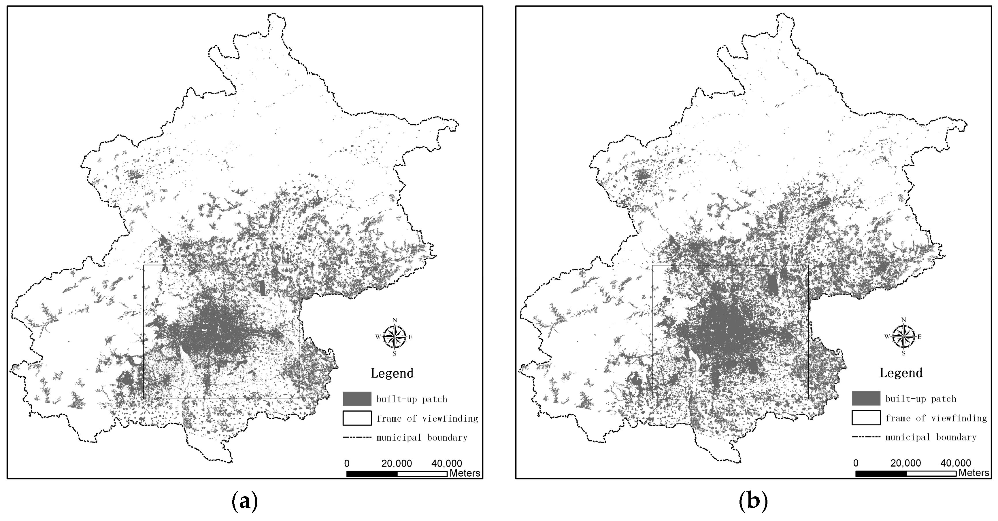
Figure 3.
A sketch map of the functional box-counting method for spatial entropy and fractal dimension measurement (first three steps). (a) The first step; (b) The second step; (c) The third step.
Figure 3.
A sketch map of the functional box-counting method for spatial entropy and fractal dimension measurement (first three steps). (a) The first step; (b) The second step; (c) The third step.
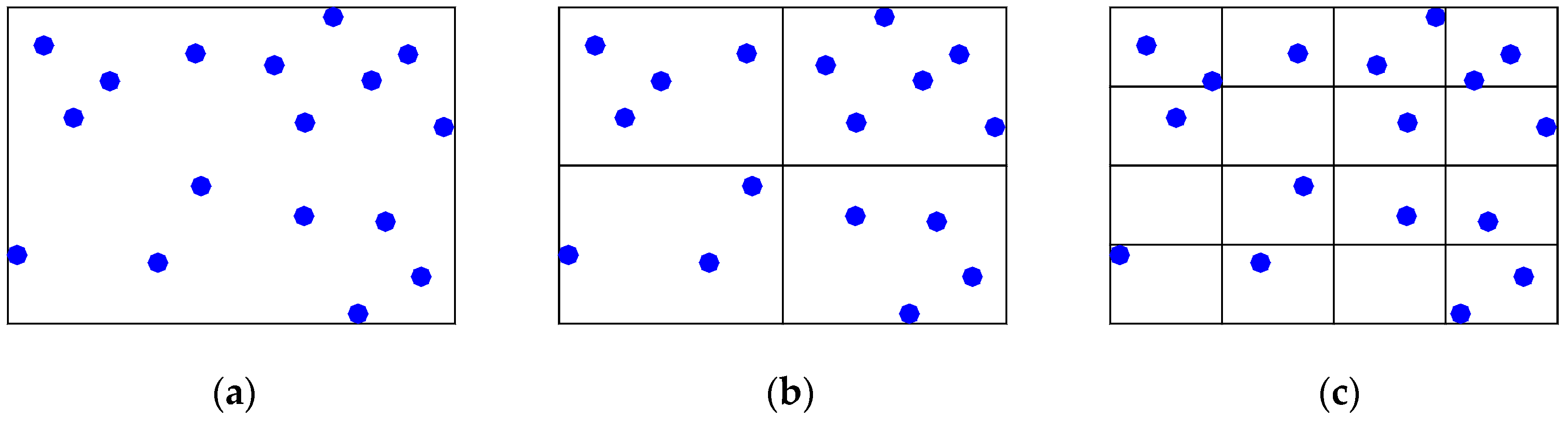
Figure 4.
The plots for evaluating multifractal parameters of Beijing’s urban form and growth patterns (2006). (a) Capacity dimension (q = 0, D0); (b) Information dimension (q = 1, D1); (c) Correlation dimension (q = 2, D2).
Figure 4.
The plots for evaluating multifractal parameters of Beijing’s urban form and growth patterns (2006). (a) Capacity dimension (q = 0, D0); (b) Information dimension (q = 1, D1); (c) Correlation dimension (q = 2, D2).
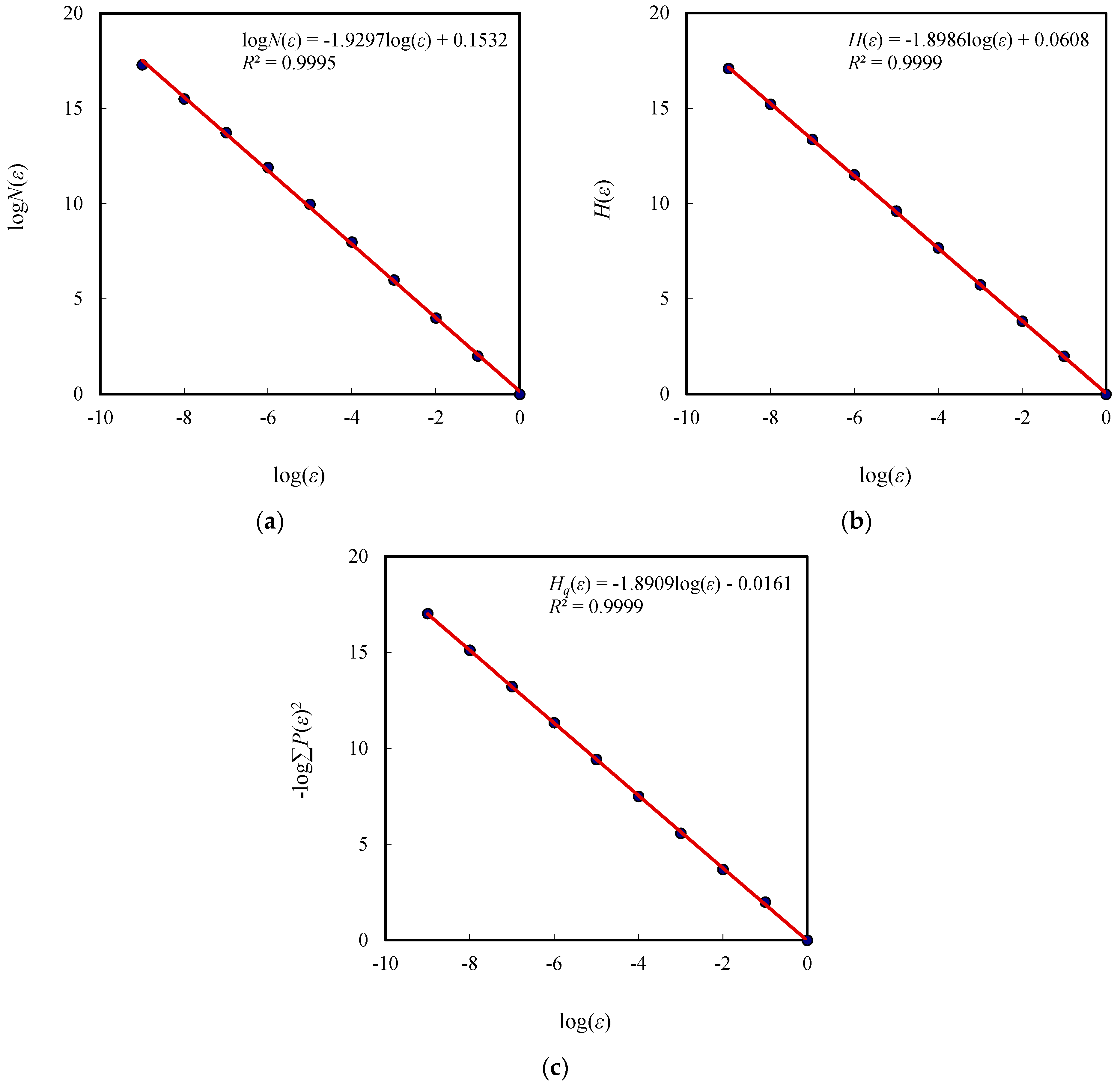
Figure 5.
The linear relationships between fractal dimension values and the corresponding entropy values (based on the linear size 1/29) of Beijing’s urban form (1988–2009). (a) Capacity dimension D0 and macro state entropy S = M0; (b) Information dimension D1 and Shannon entropy H = M1; (c) Correlation dimension D2 and the second order Renyi entropy M2.


Figure 6.
Two sketched maps of Hangzhou’s urban form and growth. (a) Urban pattern in 1980; (b) Urban pattern in 1996.
Figure 6.
Two sketched maps of Hangzhou’s urban form and growth. (a) Urban pattern in 1980; (b) Urban pattern in 1996.
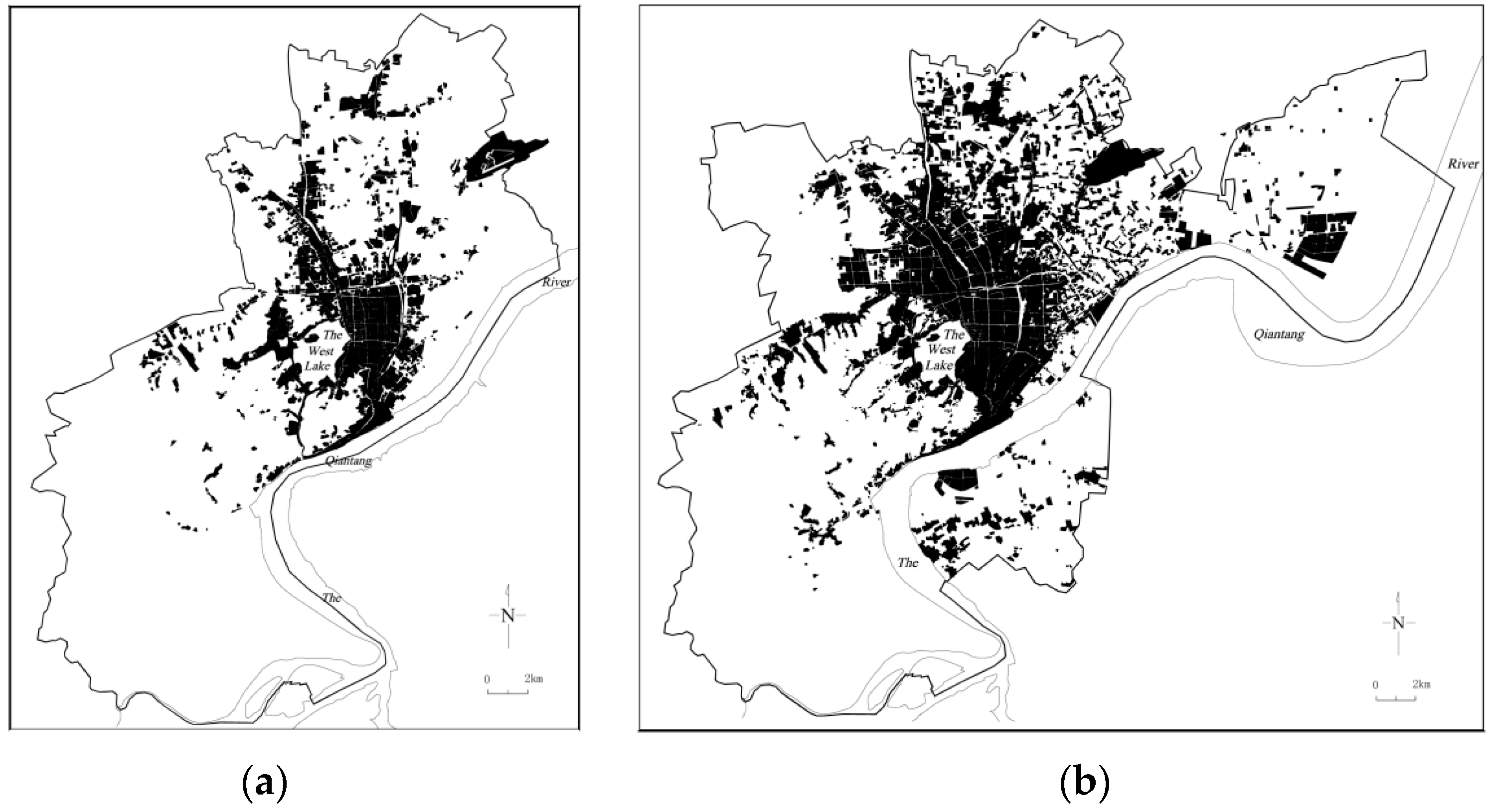
Figure 7.
The linear relationships between capacity dimension values and the macro state entropy values (based on the linear size 1/29) of Hangzhou’s urban form (1949–1996). (a) The linear size of box is too large, i.e., ε = 1/21, so the statistical correlation cannot appear; (b) The box size is small enough, i.e., ε = 1/29, and the linear correlation becomes very clear.

Table 1.
Entropy and fractal dimension of the box fractal based on different scales of measurement.
| Step m | Linear Size of Fractal Copies εm | Number of Fractal Copies Nm(ε) | Entropy H (nat) | Fractal Dimension D |
|---|---|---|---|---|
| 1 | 1/30 | 50 | 0.000 | (0, or 2) |
| 2 | 1/31 | 51 | 1.609 | 1.465 |
| 3 | 1/32 | 52 | 3.219 | 1.465 |
| 4 | 1/33 | 53 | 4.828 | 1.465 |
| 5 | 1/34 | 54 | 6.438 | 1.465 |
| 6 | 1/35 | 55 | 8.047 | 1.465 |
| 7 | 1/36 | 56 | 9.657 | 1.465 |
| 8 | 1/37 | 57 | 11.266 | 1.465 |
| 9 | 1/38 | 58 | 12.876 | 1.465 |
| 10 | 1/39 | 59 | 14.485 | 1.465 |
| … | … | … | … | … |
| m | 1/3m−1 | 5m−1 | (m − 1)ln(5) | ln(5)/ln(3) |
Table 2.
The state entropy, information entropy, and Renyi entropy of Beijing’s urban form.
| Scale (ε) | Three Types of Entropy Values (Mq) | ||||||||||||||
|---|---|---|---|---|---|---|---|---|---|---|---|---|---|---|---|
| 1988 | 1992 | 1999 | 2006 | 2009 | |||||||||||
| M0 (q = 0) | M1 (q = 1) | M2 (q = 2) | M0 (q = 0) | M1 (q = 1) | M2 (q = 2) | M0 (q = 0) | M1 (q = 1) | M2 (q = 2) | M0 (q = 0) | M1 (q = 1) | M2 (q = 2) | M0 (q = 0) | M1 (q = 1) | M2 (q = 2) | |
| 1/20 | 0.0000 | 0.0000 | 0.0000 | 0.0000 | 0.0000 | 0.0000 | 0.0000 | 0.0000 | 0.0000 | 0.0000 | 0.0000 | 0.0000 | 0.0000 | 0.0000 | 0.0000 |
| 1/21 | 2.0000 | 1.9672 | 1.9364 | 2.0000 | 1.9775 | 1.9569 | 2.0000 | 1.9650 | 1.9279 | 2.0000 | 1.9964 | 1.9928 | 2.0000 | 1.9942 | 1.9886 |
| 1/22 | 4.0000 | 3.5770 | 3.2749 | 4.0000 | 3.4693 | 3.1363 | 4.0000 | 3.6850 | 3.4668 | 4.0000 | 3.8306 | 3.6976 | 4.0000 | 3.9231 | 3.8617 |
| 1/23 | 6.0000 | 5.3986 | 5.0152 | 6.0000 | 5.2657 | 4.8831 | 6.0000 | 5.5608 | 5.2991 | 6.0000 | 5.7431 | 5.5816 | 6.0000 | 5.8783 | 5.7959 |
| 1/24 | 7.9944 | 7.2654 | 6.8736 | 7.9887 | 7.1303 | 6.7571 | 7.9887 | 7.4614 | 7.1875 | 7.9887 | 7.6778 | 7.5024 | 7.9944 | 7.8342 | 7.7421 |
| 1/25 | 9.9233 | 9.1260 | 8.7581 | 9.9672 | 9.0084 | 8.6618 | 9.9556 | 9.3590 | 9.0951 | 9.9672 | 9.6112 | 9.4351 | 9.9701 | 9.7897 | 9.6896 |
| 1/26 | 11.7224 | 10.9502 | 10.6430 | 11.8986 | 10.8623 | 10.5656 | 11.8431 | 11.2301 | 10.9973 | 11.8986 | 11.5117 | 11.3460 | 11.9263 | 11.7163 | 11.6131 |
| 1/27 | 13.3201 | 12.7152 | 12.4926 | 13.7249 | 12.6723 | 12.4488 | 13.5868 | 13.0592 | 12.8761 | 13.7249 | 13.3678 | 13.2316 | 13.8404 | 13.6112 | 13.5160 |
| 1/28 | 14.9124 | 14.4897 | 14.3423 | 15.5017 | 14.4859 | 14.3320 | 15.2798 | 14.8915 | 14.7582 | 15.5017 | 15.2185 | 15.1195 | 15.7081 | 15.4972 | 15.4202 |
| 1/29 | 16.5871 | 16.3073 | 16.2155 | 17.2877 | 16.3234 | 16.2255 | 17.0079 | 16.7416 | 16.6532 | 17.2877 | 17.0879 | 17.0245 | 17.5632 | 17.3994 | 17.3428 |
Note: The base of the logarithm is 2, thus the unit of information quantity is bit. If a calculation is based on natural base of logarithm, all these values should be multiplied by ln(2).
Table 3.
The capacity dimension, information dimension, and correlation dimension of Beijing’s urban form and the related statistics.
Table 3.
The capacity dimension, information dimension, and correlation dimension of Beijing’s urban form and the related statistics.
| Type | Parameter/Statistic | 1988 | 1992 | 1999 | 2006 | 2009 |
|---|---|---|---|---|---|---|
| Capacity dimension D0 | Parameter D0 | 1.8507 | 1.8584 | 1.8998 | 1.9297 | 1.9575 |
| Standard error δ | 0.0310 | 0.0299 | 0.0222 | 0.0160 | 0.0095 | |
| R Square R2 | 0.9978 | 0.9979 | 0.9989 | 0.9995 | 0.9998 | |
| Information dimension D1 | Parameter D1 | 1.8099 | 1.8130 | 1.8602 | 1.8986 | 1.9335 |
| Standard error δ | 0.0070 | 0.0114 | 0.0050 | 0.0053 | 0.0051 | |
| R Square R2 | 0.9999 | 0.9997 | 0.9999 | 0.9999 | 0.9999 | |
| Correlation dimension D2 | Parameter D2 | 1.8039 | 1.8071 | 1.8530 | 1.8909 | 1.9259 |
| Standard error δ | 0.0201 | 0.0271 | 0.0130 | 0.0065 | 0.0027 | |
| R Square R2 | 0.9990 | 0.9982 | 0.9996 | 0.9999 | 1.0000 |
Note: These fractal parameters represent three typical fractal dimensions in a global multifractal dimension spectrum [24]. The R2 values reflect the correlation between the natural logarithm of the linear sizes, ln(ε), and the corresponding Renyi entropy.
Table 4.
The squared coefficients of correlation between fractal dimension values and the corresponding entropy values of Beijing’s urban form (1988–2009).
Table 4.
The squared coefficients of correlation between fractal dimension values and the corresponding entropy values of Beijing’s urban form (1988–2009).
| Moment Order q | Correlation Coefficient Square (R2) | ||||||||
|---|---|---|---|---|---|---|---|---|---|
| ε = 1/21 | ε = 1/22 | ε = 1/23 | ε = 1/24 | ε = 1/25 | ε = 1/26 | ε = 1/27 | ε = 1/28 | ε = 1/29 | |
| q = 0 | -- | -- | -- | 0.0095 | 0.9330 | 0.9786 | 0.9963 | 1.0000 | 0.9990 |
| q = 1 | 0.5909 | 0.9460 | 0.9549 | 0.9641 | 0.9768 | 0.9877 | 0.9963 | 0.9994 | 0.9999 |
| q = 2 | 0.5460 | 0.9640 | 0.9780 | 0.9846 | 0.9893 | 0.9925 | 0.9966 | 0.9989 | 0.9996 |
Note: If q = 0, the first three square correlation coefficient values cannot be calculated.
Table 5.
The macro state entropy, capacity dimension, and the squared coefficient of correlation between the fractal dimension and entropy of Hangzhou’s urban form (1949–1996).
Table 5.
The macro state entropy, capacity dimension, and the squared coefficient of correlation between the fractal dimension and entropy of Hangzhou’s urban form (1949–1996).
| Type | Box Size | Parameter and Statistic | R Square R2 | |||
|---|---|---|---|---|---|---|
| 1949 | 1959 | 1980 | 1996 | |||
| Entropy | 1/21 | 1.3863 | 1.3863 | 1.3863 | 1.3863 | -- |
| 1/22 | 2.7081 | 2.7081 | 2.7726 | 2.7726 | 0.8992 | |
| 1/23 | 3.6376 | 3.7842 | 4.1431 | 4.1431 | 0.9812 | |
| 1/24 | 4.3820 | 4.7536 | 5.4161 | 5.4765 | 0.9943 | |
| 1/25 | 5.3132 | 5.8201 | 6.6631 | 6.7979 | 0.9981 | |
| 1/26 | 6.3244 | 6.9048 | 7.8793 | 8.0983 | 0.9997 | |
| 1/27 | 7.3896 | 8.0446 | 9.1344 | 9.2927 | 0.9975 | |
| 1/28 | 8.5704 | 9.2595 | 10.3984 | 10.6780 | 0.9999 | |
| 1/29 | 9.8901 | 10.5666 | 11.6846 | 11.9757 | 0.9999 | |
| Capacity dimension | Parameter D0 | 1.5013 | 1.6379 | 1.8581 | 1.9115 | |
| R Square R2 | 0.9953 | 0.9983 | 0.9995 | 0.9997 | ||
| Standard error δ | 0.0365 | 0.0236 | 0.0148 | 0.0112 | ||
| Eigen entropy | Parameter b | 0.6630 | 0.6095 | 0.5379 | 0.5230 | |
| R Square R2 | 0.9953 | 0.9983 | 0.9995 | 0.9997 | ||
| Entropy 1/b | 1.5084 | 1.6406 | 1.8591 | 1.9120 | ||
Note: In the last column, the values of R2 refer to the squared coefficient of correlation between fractal dimension and entropy based on different linear sizes of boxes; in the last sixth rows, the values of R2 denote the goodness of fit for estimating the fractal dimension. Differing from Feng and Chen [44], the scaling range is not considered for fractal dimension evaluation in this paper.
Table 6.
The information entropy of urban population density and the related measurements of Hangzhou (1964–2000).
Table 6.
The information entropy of urban population density and the related measurements of Hangzhou (1964–2000).
| Year | Average Density (ρ) | Characteristic Radius (r0) | Entropy (H) | Entropy Ratio (H/Hmax) |
|---|---|---|---|---|
| 1964 | 4721.3643 | 3.5644 | 2.4593 | 0.7548 |
| 1982 | 5702.7587 | 3.6713 | 2.4843 | 0.7625 |
| 1990 | 6774.3742 | 3.6285 | 2.5486 | 0.7822 |
| 2000 | 8411.6099 | 3.9457 | 2.7251 | 0.8364 |
Table 7.
The characteristic values of spatial entropy (1/b) and the corresponding fractal dimension values (Dq).
Table 7.
The characteristic values of spatial entropy (1/b) and the corresponding fractal dimension values (Dq).
| Year | a | b | R2 | 1/b | Dq |
|---|---|---|---|---|---|
| 1988 | 1.1183 | 0.5391 | 0.9978 | 1.8549 | 1.8507 |
| 1.0132 | 0.5525 | 0.9999 | 1.8101 | 1.8099 | |
| 0.9367 | 0.5538 | 0.9990 | 1.8057 | 1.8039 | |
| 1992 | 1.1122 | 0.5370 | 0.9979 | 1.8622 | 1.8584 |
| 0.9842 | 0.5514 | 0.9997 | 1.8136 | 1.8130 | |
| 0.9088 | 0.5524 | 0.9982 | 1.8103 | 1.8071 | |
| 1999 | 1.0787 | 0.5258 | 0.9989 | 1.9018 | 1.8998 |
| 1.0089 | 0.5375 | 0.9999 | 1.8603 | 1.8602 | |
| 0.9577 | 0.5395 | 0.9996 | 1.8537 | 1.8530 | |
| 2006 | 1.0547 | 0.5179 | 0.9995 | 1.9308 | 1.9297 |
| 1.0222 | 0.5267 | 0.9999 | 1.8987 | 1.8986 | |
| 0.9938 | 0.5288 | 0.9999 | 1.8911 | 1.8909 | |
| 2009 | 1.0324 | 0.5108 | 0.9998 | 1.9578 | 1.9575 |
| 1.0229 | 0.5172 | 0.9999 | 1.9336 | 1.9335 | |
| 1.0109 | 0.5192 | 1.0000 | 1.9260 | 1.9259 |
Note: Before making the least squares regression, all the entropy values on the base of 2 in Table 2 have been transformed into the entropy values on the natural base, e. The characteristic values of spatial entropy, 1/b, is close to the fractal dimension values, Dq.
Table 8.
A comparison between entropy meaning and fractal dimension meaning.
| Type | Entropy | Fractal Dimension |
|---|---|---|
| Distribution | Gaussian (normal) distribution | Pareto-Mandelbrot (power-law) distribution |
| Scale | Based on characteristic scale | Based on scaling (scale-free) |
| System | Determinate systems | Complex systems |
| Symmetry | Spatio-temporal translational symmetry | Scaling symmetry (invariance under contraction or dilation) |
| Variation | Different types of entropy | Different types of fractal dimension |
| State | Order or chaos | Edge of chaos |
| Spatial measurement | The results depend on the method, the scope of the study area, and the linear size | The results depend on the method and the scope of the study area, but not on the linear size |
| Sphere of application | (1) The patterns and processes with characteristic scale (determinate length, size, mean, eigen value ); (2) Global analysis | (1) The patterns and processes without characteristic scale (indeterminate length, size, mean, eigen value ); (2) Both global and local analysis. |
| Example 1 | Urban population density (Table 6) | Urban land use pattern (Table 4 and Table 5) |
| Example 2 | Size distributions of road lengths | Urban traffic network |
| Example 3 | Lognormal distribution of city size | Power-law distribution of city size |
© 2017 by the authors. Licensee MDPI, Basel, Switzerland. This article is an open access article distributed under the terms and conditions of the Creative Commons Attribution (CC BY) license (http://creativecommons.org/licenses/by/4.0/).
Share and Cite
MDPI and ACS Style
Chen, Y.; Wang, J.; Feng, J. Understanding the Fractal Dimensions of Urban Forms through Spatial Entropy. Entropy 2017, 19, 600. https://doi.org/10.3390/e19110600
AMA Style
Chen Y, Wang J, Feng J. Understanding the Fractal Dimensions of Urban Forms through Spatial Entropy. Entropy. 2017; 19(11):600. https://doi.org/10.3390/e19110600
Chicago/Turabian StyleChen, Yanguang, Jiejing Wang, and Jian Feng. 2017. "Understanding the Fractal Dimensions of Urban Forms through Spatial Entropy" Entropy 19, no. 11: 600. https://doi.org/10.3390/e19110600
Note that from the first issue of 2016, this journal uses article numbers instead of page numbers. See further details here.