Rate Distortion Functions and Rate Distortion Function Lower Bounds for Real-World Sources

Department of Electrical and Computer Engineering, University of California, Santa Barbara, CA 93106-9560, USA
Entropy 2017, 19(11), 604; https://doi.org/10.3390/e19110604
Submission received: 27 September 2017
/
Revised: 3 November 2017
/
Accepted: 6 November 2017
/
Published: 11 November 2017
(This article belongs to the Special Issue Rate-Distortion Theory and Information Theory)
Abstract
:Although Shannon introduced the concept of a rate distortion function in 1948, only in the last decade has the methodology for developing rate distortion function lower bounds for real-world sources been established. However, these recent results have not been fully exploited due to some confusion about how these new rate distortion bounds, once they are obtained, should be interpreted and should be used in source codec performance analysis and design. We present the relevant rate distortion theory and show how this theory can be used for practical codec design and performance prediction and evaluation. Examples for speech and video indicate exactly how the new rate distortion functions can be calculated, interpreted, and extended. These examples illustrate the interplay between source models for rate distortion theoretic studies and the source models underlying video and speech codec design. Key concepts include the development of composite source models per source realization and the application of conditional rate distortion theory.
1. Introduction
Shannon introduced the concept of a rate distortion function for a specified source model and distortion measure that defines the optimal performance theoretically attainable (OPTA) by any codec, of any cost and complexity, when coding the specified source according to the chosen distortion measure [1,2]. Shannon’s goal was to provide a fundamental limit on performance that would serve as a motivating goal in source codec design and that would allow researchers and engineers to evaluate how close existing codec designs are to this optimal performance. If the codecs were far away from the performance bound set by the rate distortion function, then more work was needed; however, if the current codec performance was close to the bound, an informed decision could be made as to whether further work was warranted and worth the effort, and perhaps the additional complexity.
The central roles of the source model and of the fidelity criterion are obvious from the definition of the rate distortion function, and researchers realized very quickly that finding rate distortion functions for real sources, such as voice and video, and for practically meaningful distortion measures would be a difficult challenge [3,4,5]. Their recognition was that real-world sources are complex and finding parsimonious source models that captured the essential elements of a real-world source would be difficult to find. Similarly, it was recognized that the fidelity criterion needs to encompass what is important to the user yet still be analytically tractable. More specifically, for voice compression, the fidelity criterion needs to provide an objective measure of the subjective quality and of the intelligibility of the compressed voice signal as discerned by a listener; and for video, the fidelity criterion needs to associate a quantitative value to the quality of the coded video as determined by a viewer.
Interestingly, considerable progress has been made. The author and his students recognized that the source models should be a composite source model consisting of several different modes and that, in order to obtain a lower bound, the source model needs to be per realization of the source sequence rather than an average model over many different realizations. This idea is similar to the collections of models idea for compression algorithm design discussed by Effros [6]. Second, the squared error fidelity criterion was adopted and established to be perceptually meaningful through mappings for voice and standard practice for video. Third, conditional rate distortion theory, as developed by Gray [7], was used in concert with the composite source models. Many of the results are collected in the monograph coauthored by Gibson and Hu [8], wherein rate distortion bounds are exhibited that lower bound the performance of the best known voice and video codecs.
However, unlike the case of an i.i.d. Gaussian source subject to the mean squared error distortion measure, we do not have the rate distortion functions for voice and video set in stone. That is, the rate distortion functions produced thus far for voice and video in [8] are based on the source model structures developed at that time. Since voice and video are complex collections of sources, these prior models can be improved. If this is so, will the rate distortion functions produced in Gibson and Hu [8] lower bound the rate distortion performance of all future voice and video codecs? The answer is “Almost certainly not!” So, how should the existing results be interpreted and what are their implications? Does this mean that rate distortion theory is not relevant to real-world, physical sources? And, can rate distortion bounds play a role in codec design? These are the questions addressed in this paper.
These discussions point out the interesting interplay between rate distortion functions and source codec design, which we also develop in detail here. In particular, we note that rate distortion functions exhibit the role and structure of the source models being used to obtain these performance bounds; and further, since codecs for real-world sources are based on models themselves, the rate distortion performance of a codec based on a specific source model can be determined without implementing the codec itself by using rate distortion theory! This latter observation thus can remove some uncertainty in a complex step in source codec design. More specifically, if the rate distortion function for a new source model shows significant gains in performance, researchers and designers can move forward with codec designs based on this model knowing two things: (1) There is worthwhile performance improvement available, and (2) if the codec components are properly designed, this performance can be achieved.
We begin with Section 2, discussing key points for the development of good source models, and Section 3 which discusses the relationship between the squared error distortion measure, that is often used for tractability in rate distortion theoretic calculations, and real-world perceptual distortion measures for video and speech. Section 4 then briefly states the basic definitions from rate distortion theory needed in the paper, followed by several subsections summarizing key well-known results from rate distortion theory. In particular, Section 4.1 presents the rate distortion function for memoryless Gaussian sources and the mean squared error distortion measure, Section 4.2 outlines the powerful technique of reverse water-filling for evaluating rate distortion functions of Gaussian sources as the distortion constraint is adjusted, and Section 4.3 presents the corresponding basic theoretical result for Gaussian autoregressive processes, including the autoregressive lower bound to the rate distortion function. Section 4.4 then builds on the rate distortion developments in prior sections and states the needed results from conditional rate distortion theory that are essential in subsequent rate distortion function calculations for video and speech. Section 4.5 and Section 4.6 present the Shannon lower bound and the Wyner–Ziv lower bound, respectively, to the rate distortion function, and discuss when these lower bounds coincide with each other and with the autoregressive lower bound. The theoretical rate distortion performance bound associated with a given source codec structure is discussed in Section 5, and the more familiar concept of the operational rate distortion performance for a codec is presented in Section 6. We then turn our attention to the development of rate distortion functions for video in Section 7, where we build the required composite source models, and in Section 8, where we compare and contrast the rate distortion bounds for the several video source models. We follow this with the development of composite autoregressive source models for speech in Section 9 and then the calculation of the rate distortion functions for the various composite speech models are presented and contrasted in Section 10. Section 11 puts all of the prior results in context and clearly describes how rate distortion functions, and the models upon which they are based, can be used in the codec design process and for codec performance prediction and evaluation.
2. Source Models
In rate distortion theory, a source model, such as memoryless Gaussian or autoregressive, is assumed and that model is both accurate and fixed for the derivation of the rate distortion function. For this particular source model and a chosen distortion measure, the rate distortion function is a lower bound on the best performance achievable by any source codec for that source and distortion measure. For real-world sources, the source usually cannot be modeled exactly. However, for a given source sequence, we can develop approximate models based on our understanding of the source and signal processing techniques.
Coding systems such as vector quantizers (VQs) are designed by minimizing the distortion averaged over a training set, which is a large set of source sequences that are (hopefully) representative of the source sequences to be coded. The result is a codec that performs well on the average, but for some sequences, may not perform well–that is, may perform poorer than average. In contrast, rate distortion theory is concerned with finding a lower bound on the performance of all possible codecs designed for a source. As a result, the interest is not in a rate distortion curve based on a source model averaged over a large class of source realizations, but the interest is in a very accurate model for a very specific source realization.
Therefore, in order to obtain a lower bound on the rate distortion performance for a given distortion measure, we develop models for individual realizations of the source, such as the individual sequences used to train the VQs. Then, we compare the resulting rate distortion function to the performance of the best known codecs on that sequence. We see that as we make the model more accurate, we can get very interesting and important performance bounds.
An immediate question that arises is, what if the few source realizations we choose to explore are difficult to code or easy to code? To circumvent the misleading results possible from such scenarios, it is necessary to select a method to get an aggregate optimum performance attainable over a large set of realizations. There are many ways to do this. One way would be to calculate the difference in average distortion at a given desirable distortion level between the rate distortion function and the best codec performance for each realization and average these differences. A similar process could be followed for a chosen desired rate. Another approach would be to calculate the average difference in mean squared error over all rates of interest for each realization, similar to the Bjontegaard Peak Signal-to-Noise Ratio (PSNR) [9], and then average these values for all realizations. Yet another approach would be to create histograms of the differences in distortion between and the codec performance per realization over all values of distortion of interest compiled over all realizations.
One can see many valid ways to aggregate the results and still work with the rate distortion function as the best performance theoretically attainable for each individual realization. In this paper, we do not perform aggregation as that is quite dependent on preferences and goals. What we do here is demonstrate the calculation of for models of real-world sources, illustrate the criticality of good source models, and provide insight into how to interpret and extend the results.
3. Distortion Measures
We utilize single-letter squared error as the distortion measure throughout this paper [10]. Practitioners in video and speech coding have long pointed out that the compressed source is being delivered to a human user and so it is the perceptual quality of the reconstructed source as determined by a human user that should be measured, not per letter squared error. This observation is, of course, true. Interestingly, however, still image and video codec designers have discovered that single letter difference distortion measures, such as the mean squared error or the sum of the absolute values of the differences between the input samples and the corresponding reconstructed samples, are important and powerful tools for codec design and performance evaluation [9]. For video, subjective studies are also commonly performed after the objective optimization has been completed. These subjective studies provide additional insights into the codec performance but do not invalidate these difference distortion measures as design tools.
For speech coding, objective measures that model the perceptual process of human hearing have been developed and these software packages are widely accepted for speech codec performance evaluation and design [11,12]. After the design process has been completed, just as in the video case, subjective testing is performed with human subjects. Although we use the mean squared error for rate distortion function development, a mapping procedure has been devised that takes the mean squared error based rate distortion functions and maps them into a more perceptually meaningful rate distortion bound. These details are left to the references [8]. Therefore, the rate distortion functions can be found using the per letter squared error distortion measure, and then the average distortion for each rate can be mapped into a perceptually meaningful quantity, namely, the (Wideband) Perceptual of Speech Quality Mean Opinion Score ((W)PESQ-MOS) [11,12]. Again, with this mapping, we see the power of the squared error distortion measure in evaluating and bounding speech codec performance.
4. Rate Distortion Theory
In this section and its’ several subsections, we summarize well-known results from the rate distortion theory literature to set the stage for the developments that follow. We begin with the basic definitions and establish notation.
For a specific source model and distortion measure, rate distortion theory answers the following fundamental question: What is the minimum number of bits (per data sample) needed to represent the source at a chosen average distortion irrespective of the coding scheme and complexity? A mathematical characterization of the rate distortion function is given by the following fundamental theorem of rate distortion theory [1,2].
Theorem 1 (Shannon’s third theorem).
The minimum achievable rate to represent an i.i.d. source X with a probability density function , by , with a bounded distortion function such that , is equal to
where is the mutual information between X and .
The rate distortion function is appropriate when we want to minimize the rate subject to a constraint on distortion. This approach is of interest in those problems where rate can be variable but the specified distortion is the critical parameter. The most common examples of this class of problems are those which require perceptually “transparent” reproduction of the input source, such as high quality audio or high resolution video.
There is another class of problems, however, which are of practical interest, such as those where the maximum rate is specified but the distortion may be at some acceptable level above transparent. In these cases, the problem can be posed as minimizing the distortion for a given constraint on rate. Mathematically, we can pose the problem as [14].
Theorem 2.
For an i.i.d. source X with a probability density function , the minimum average distortion achievable by a reconstruction with chosen such that the rate , is equal to
where is the mutual information between X and .
This function, , is called the Distortion Rate function and is appropriate for problems such as voice and video coding for fixed bandwidth channels as allocated in wireless applications.
Whether or not there exists a closed-form rate distortion function depends on the distribution of the source and the criterion selected to measure the fidelity of reproduction between the source and its reconstruction.
4.1. Memoryless Gaussian Sources
The rate distortion function for a scalar Gaussian random variable with squared error distortion measure is [10]
The distortion rate function for a scalar Gaussian random variable with squared error distortion measure is
Shannon introduced a quantity called the entropy rate power in his original paper, The Mathematical Theory of Communication [1], which he defined as the power in a Gaussian source with the same differential entropy as the original process. What this means is that given any random process Y, possibly non-Gaussian, with differential entropy, say , the corresponding entropy rate power, also called entropy power, is given by
Shannon also showed that the rate distortion function for the process Y is bounded as
where is the variance of the source and Q is the entropy power of the source.
The bounds in Equation (6) are critically important in the field of rate distortion theory. The lower bound involving the entropy rate power is explored in several ways in subsequent sections. The upper bound is important because it says that, for the squared error distortion measure, the Gaussian source is the worst case source in that its rate distortion performance is worse than any other source. Thus, if we calculate the rate distortion function for a Gaussian source, we have a lower bound on the best rate distortion performance of the source that is the most pessimistic possible. Therefore, if the resulting rate distortion function shows that improved performance can be obtained for a particular codec, we know that at least that much performance improvement is possible. Alternatively, if the codec performance is close to the Gaussian-assumption bound or below it, we know that the Gaussian assumption may not provide any insights into the best rate distortion performance possible for that source and distortion measure.
However, what we will see is that the Gaussian-assumption rate distortion function is extraordinarily useful in providing practical and insightful rate distortion bounds for real-world sources.
4.2. Reverse Water-Filling
The rate distortion function of a vector of independent (but not identically distributed) Gaussian sources is calculated by the reverse water-filling theorem [13]. This theorem says that one should encode the independent sources with equal distortion level , as long as does not exceed the variance of the transmitted sources, and that one should not transmit at all those sources whose variance is less than the distortion . The rate distortion function is traced out as is varied from 0 up to the largest variance of the sources.
Theorem 3 (Reverse water-filling theorem).
For a vector of independent random variables such that and the distortion measure , the rate distortion function is
where
Proof.
See [13]. ☐
Several efforts have avoided the calculation of the rate distortion function as is varied by considering only the small distortion case, which is when is less than the smallest variance of any of the components [16,17,18,19,20]. Prior results trace out the rate distortion function as the distortion or slope related parameter is varied across all possible values. The small distortion lower bounds avoid these calculations, and it is thus of interest to investigate how tight these small distortion bounds are for rate/distortion pairs of practical importance. For the case where distortion is small in the sense that for all i, then
where is the correlation matrix of the source.
This approach has been widely used in different rate distortion performance calculations and we investigate here whether it is successful in providing a useful lower bound for all distortion/rate pairs.
4.3. Rate Distortion Function for a Gaussian Autoregressive Source
Since Shannon’s rate distortion theory requires an accurate source model and a meaningful distortion measure, and both of these are difficult to express mathematically for real physical sources such as speech, these requirements have limited the impact of rate distortion theory on the lossy compression of speech. There have been some notable advances and milestones, however. Berger [10] and Gray [21], in separate contributions in the late 60’s and early 70’s, derived the rate distortion function for Gaussian autoregressive (AR) sources for the squared error distortion measure. Since the linear prediction model, which is an AR model, has played a major role in voice codec design for decades and continues to do so, their results are highly relevant to our work.
The basic result is summarized in the following theorem [10]:
Theorem 4.
Let be an mth-order autoregressive source generated by an i.i.d. sequence and the autoregression constants Then the mean squared error (MSE) rate distortion function of is given parametrically by
and
where
The points on the rate distortion function are obtained as the parameter is varied from the minimum (essential infimum) to the maximum (essential supremum) of the power spectral density of the source. can be associated with a value of the average distortion, and only the shape of the power spectral density, , above the value of is reproduced at the corresponding distortion level. is related to the average distortion through the slope of the rate distortion function at the point where the particular average distortion is achieved. This idea proves important later when we work with composite source models.
If , then and the rate distortion function is
where Q is the entropy rate power of the source [10] as defined in Equation (5). The subscript parameter is usually suppressed.
The importance of this theorem is that autoregressive sources have played a principal role in the design of leading narrowband and wideband voice codecs for decades. The rate distortion function in this theorem offers a direct connection to these codecs, although as we shall demonstrate in the following, one single AR source model will not do.
4.4. Rate Distortion Bounds for Composite Source Models
Composite source models, which combine multiple subsources according to a switch process [22,23,24,25] can serve as a good source model for video [26,27] when characterizing achievable rate distortion performance. Given a general composite source model, a rate distortion bound based on the MSE distortion measure can be derived [28] using the conditional rate distortion results from Gray [29]. The conditional rate distortion function of a source with side information Y, which serves as the subsource information, is defined as
where
It can be proved [29] that the conditional rate distortion function in Equation (14) can also be expressed as
and the minimum is achieved by adding up the individual, also called marginal, rate-distortion functions at points of equal slopes of the marginal rate distortion functions. Utilizing the classical results for conditional rate distortion functions in Equation (16), the minimum is achieved at ’s where the slopes are equal for all y and .
This conditional rate distortion function can be used to write the following inequality involving the overall source rate distortion function [29]
where is the mutual information between and Y. We can bound by
where K is the number of subsources and M is the number of pixels representing how often the subsources change in the video sequence. If K is relatively small and M is on the order of 10 times larger or more, the second term on the right in Equation (17) is negligible, and the rate distortion for the source is very close to the conditional rate distortion function in Equation (16).
4.5. The Shannon Lower Bound
In Shannon’s seminal paper on rate distortion theory [2], he realized that for many source models and distortion measures, the solution of the constrained optimization problem defining would be difficult to obtain, so he derived what has come to be known as the Shannon Lower Bound (SLB) to . Specifically, for a random variable X with continuous probability density function , and for a difference distortion measure , he derived the lower bound to , denoted given by [2]
where is the set of all probability densities such that .
A generalized version of the SLB has been obtained by Berger [10] for stationary processes specialized to the squared-error distortion measure, called the generalized Shannon Lower Bound, as
where is the entropy rate of the process and D is the average distortion. Note that for a Gaussian source, , the lower bound in Equation (6).
If we let the that maximizes be , then we can write the SLB as
and it can be shown that if and only if
where is the probability density function of the reconstructed source. Recognizing that the convolution of the probability density functions of two statistically independent random variables is the probability density of their sum, we see that this result implies that , where Z is the reconstruction error and is statistically independent of . This expression has been called the Shannon Backward Channel [10].
4.6. The Wyner–Ziv Lower Bound
Wyner and Ziv [30] derived a lower bound to the rate distortion function for stationary sources in terms of the rate of the memoryless source with the same marginal statistics as
where is the rate distortion function of the memoryless source and is the limit of a relative entropy. For a Gaussian source, the limit of the relative entropy is
where is the power spectral density of the source.
5. Theoretical Rate-Distortion Performance of a Specific Codec Structure
There is another set of rate distortion bounds that are sometimes of interest. These bounds are determined by considering a specific codec, determining a model for the codec operation, and using that model along with a chosen source model and distortion measure, to calculate the rate distortion function for that codec model. The result is a theoretical R-D performance bound for the codec being considered. For example, in our prior work, we examined the penalty due to blocking in video frames when coupled with optimal intra-prediction [32].
The strength of calculating this rate distortion performance bound is that the projected performance of the modeled codec can be calculated without actually implementing the codec, or if a codec implementation is available, without incurring the time and expense of actually running the codec for a wide set of input source sequences. The savings can be substantial, but as always, the accuracy of the model of the codec, the source model, and the chosen distortion measure (which must be mathematically tractable in some way) must be validated. This can only be done by comparing these codec model based performance bounds to the operational rate distortion performance of a video codec.
Some interesting prior work for multiview video coding does not assume a specific coding scheme, but obtains small distortion theoretical rate distortion performance curves when some codec structural constraints are imposed, such as the accuracy of disparity compensation and Matrix of Pictures (MOP) size. This allows the impact of these specific codec constraints on coder rate distortion performance to be investigated, which is very similar to studying the theoretical performance of a specific codec [17,18].
We denote these codec model based rate-distortion performance curves as , and for an accurate codec model with equivalent and accurate assumptions on the several source and codec model parameters,
where is the rate distortion function for the given source model and distortion measure, is the rate-distortion performance of the specific codec, and is the actual operational rate distortion curve of the specific codec. is the rate distortion curve most widely known and investigated, somewhat less so, and is the least studied rate distortion function for real video sources. The focus in this paper is on studying the unconstrained theoretical rate distortion bound, .
6. Operational Rate Distortion Functions
Operational rate distortion functions trace out the rate-distortion performance of a particular codec as the codec parameters are adjusted for a given input sequence and distortion measure. Thus, operational rate distortion functions are not theoretical bounds on performance, but operational rate distortion functions show the actual performance achievable by a codec over all codec parameter settings investigated.
Some video codecs have a built in a rate distortion optimization tool [9], which allows the codec to vary codec parameters and find the lowest coding rate subject to a constraint on the distortion, or find the smallest distortion subject to a constraint on the rate. For the former, we have
where is used to adjust the constraint on D; alternatively for the second approach,
where here is used to adjust the constraint on R.
These equations are used to help the codec achieve the lowest possible operational rate distortion function; however, there are so many video codec parameters that these optimizations are accomplished in an iterative fashion, one parameter at a time, and usually it is not practicable to consider all possible codec parameter combinations because of the enormous complexity that would be incurred [9]. We denote the operational rate distortion performance of a codec as . If the source model and distortion measure used in deriving a theoretical rate distortion bound, , are both accurate, then the theoretical will lower bound the best operational rate distortion function produced by any codec for that source and distortion measure, .
7. Image and Video Models
The research on statistically modeling the pixel values within one still image for performance analysis goes back to the 1970s where two correlation functions were proposed to model the entire image. Both assume a Gaussian distribution of zero mean and a constant variance for the pixel values.
The first correlation model is the separable model
with and denoting offsets in horizontal and vertical coordinates. The parameters and control the correlation in the horizontal and vertical directions, respectively, and their values can be chosen independently. This model was used to represent the average correlation over the entire frame. It could be calculated for different images or the parameters could be chosen to model an average over many different images [33].
The separable model had correlations that decayed too quickly in each direction so a second correlation model, called the isotropic model was proposed as
This model implies that the correlation between two pixels within an image depends only on the Euclidean distance between them [34]. The isotropic model implies that the horizontal and vertical directions have the same correlation, so the isotropic model can be generalized to obtain the model [35],
These early models found some success and provided nice insights into various studies of image compression and related performance analyses. Unfortunately, a single correlation model was often used to model an entire image or to model a set of images with the model parameters chosen to produce the best average fit over the image or set of images being modeled.
As applied to rate distortion theory, which is trying to specify the optimum performance theoretically attainable for a chosen source model and distortion measure, such average source models have several shortcomings. First, if one of these average correlation models is used as the source model in a rate distortion calculation, it is unlikely that a lower bound on the performance of different high performance codecs will be obtained. This is because most image (and video) codecs are designed to adjust their coding techniques to different regions and blocks in an image/video frame, which an average model cannot capture. This is illustrated in subsequent sections. Indeed, this limitation caused doubt as to whether rate distortion theory would even be applicable to real-world sources such as still images and video since it was felt that rate distortion theory could not capture the nonstationary behavior of real-world sources [4].
In an early, seminal, and overlooked paper, Tasto and Wintz [36] propose and evaluate decomposing an image into subsources and then developing a conditional covariance model for each subsource, each with a probability of occurrence. Based on optimizing a rate distortion expression, they classify 6 × 6 pixel blocks of an image into 3 classifications, namely, high spatial frequencies, low spatial frequencies but darker than average, and low spatial frequencies and lighter than average. They also determine that setting the probability of the three classes to be equally likely was preferred.
Hu and Gibson [37] also recognized that a conditional correlation model is required, and noted that the correlation between two pixel values should not only depend on the spatial offsets between these two pixels but also on the other pixels surrounding them. To quantify the effect of the surrounding pixels on the correlation between pixels of interest, they utilized the concept of local texture, and defined a new spatial correlation coefficient model that is dependent on the local texture [37,38,39,40]. The correlation coefficient of two pixel values with spatial offsets and within a digitized natural image or an image frame in a digitized natural video is defined as
where
and are the local textures of the blocks the two pixels are located in, and the parameters a, b, , and are functions of the local texture Y, with and .
For each local texture, the combination of the five parameters a, b, , and is selected that jointly minimizes the mean absolute error (MAE) between the approximate correlation coefficients, averaged among all the blocks in a video frame that have the same local texture, and the correlation coefficients calculated using the new model, . In [37] the optimal values of the parameters a, b, , and and their respective MAEs for different videos are compared.
For the temporal component, they also study the correlation among pixels located in nearby frames, up to 16 frames in a sequence, and conclude that the temporal correlation in a video sequence can be modeled as a first order correlation that depends only on the difference in the time of occurrence of the two frames, , where indicates the temporal difference. Combining the spatial and temporal models, they define the overall correlation coefficient model of natural videos dependent on the local texture as
where is the spatial correlation coefficient and can be calculated by averaging over all local textures y’s.
8. Rate Distortion Bounds for Video
In this section we use the conditional rate distortion theory from Section 4.4 to study the theoretical rate distortion bounds of videos based on the correlation coefficient model as defined in Equations (32)–(34) and compare these bounds to the intra-frame and inter-frame coding of AVC/H.264, the Advanced Video Codec in the H.264 standard, and to HEVC, the High Efficiency Video Codec. The results presented here are taken from the references and thus are not new [8,37,38,39,40], but the goal here is to contrast the change in the rate distortion bound as the video model is changed. These comparions allow us to interpret the various rate distortion bounds and also to point toward how new bounds can be obtained and what any new bounds might mean. These comparisons also allow us to see how rate distortion bounds can be used in video codec design.
Following Hu and Gibson [37], we construct the video source in frame k by two parts: as an M by N block (row scanned to form an by 1 vector) and as the surrounding pixels ( on the top, N to the left and the one on the left top corner, forming a by 1 vector). Therefore, the video source across a few temporal frames , , ⋯, is defined as a long vector , where
We assume that is a Gaussian random vector with memory, and all entries of are of zero mean and the same variance . The value of is different for different video sequences. The correlation coefficient between each two entries of can be calculated as discussed in the references [8].
We use Y to denote the information of local textures formulated from a collection of natural videos and Y is considered as universal side information available to both the encoder and the decoder.
To form the desired comparisons, we need the rate distortion bound without taking into account the texture as side information, which is given by
which is the minimum mutual information between the source and the reconstruction , subject to a mean square distortion measure . To facilitate the comparison with the case when side information Y is taken into account, we calculate the correlation matrix as
where the are the texture dependent correlation coefficients.
The rate distortion bound with the local texture as side information is a conditional rate distortion problem for a source with memory and from Section 4.4 is
and the minimum is achieved by adding up , the individual, also called marginal, rate-distortion functions, at points of equal slopes of the marginal rate distortion functions, i.e., when are equal for all y and . These marginal rate distortion bounds can also be calculated using the classical results on the rate distortion bound of a Gaussian vector source with memory and a mean square error criterion as reviewed in Section 4, where the correlation matrix of the source is dependent on local texture y.
From Section 4.4, we know that we can use this conditional rate distortion function to write the inequality involving the overall video rate distortion function [29]
where
where K is the number of textures and M is the number of pixels representing how often the textures change in the video sequence.
In Figure 1 we show the conditional rate distortion functions for each texture, called the marginal rate distortion functions, for the first frame of the test video paris.cif (from [8]). This plot shows that the rate distortion curves of the blocks with different local textures are very different. This result implies that one average correlation model over an entire frame will not be sufficient to give us a good lower bound on .
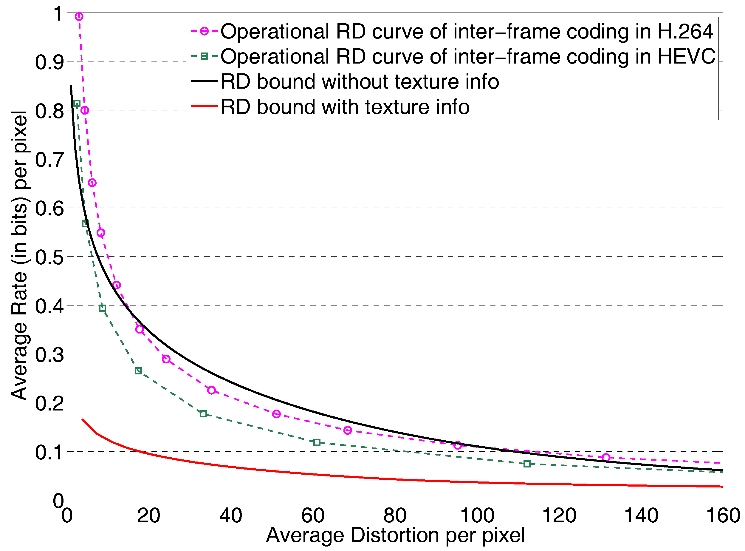
In Figure 2 we show the conditional rate distortion bound , for paris.cif and the operational rate distortion curves for paris.cif, inter-coded in AVC/H.264 and HEVC [41]. For inter-coding in H.264 and HEVC, where applicable, prediction unit sizes from to and transform unit sizes from to were allowed. The 5 frames were coded as I, B1, B0, B1, B0 where B0 is a level-0 hierarchical B frame and B1 is a a level-1 hierarchical B frame.
The rate distortion bound without local texture information, plotted as a black solid line, intersects with the actual operational rate distortion curves of H.264/AVC and HEVC, and both H.264 and HEVC have rate distortion performance curves that fall below this one average video model rate distortion curve. However, our rate distortion bounds with local texture information taken into account while making no assumptions on coding, plotted as a red solid line, is indeed a lower bound with respect to the operational rate distortion curves of both AVC/H.264 and HEVC.
The tightness of the bound and the utility in video codec design is discussed in Section 11.
9. Speech Models
Speech codec development has been greatly facilitated by a fortuitous structural match between the speech time domain waveform and the linear prediction or autoregressive model. As a result of this match, essentially all narrowband (200 Hz to 3400 Hz) and wideband (50 Hz to 7 kHz) speech codecs rely on this model [42,43]. As a consequence, using results from rate distortion theory for AR models should follow naturally. However, while AR models have been dominant in voice codec design, there are, of course, many sounds that are not well-matched by the AR model, and the codec designs adjust to compensate for these sounds in various ways. All of the successful voice codecs detect at least three different coding modes, and some codecs have attempted to switch between more than that [44,45,46,47].
More specifically, an AR process is given by
where the , are called the linear prediction coefficients for speech processing applications, and is the excitation sequence. Although in time series analysis, the excitation is often chosen to be an i.i.d. Gaussian sequence, speech modeling requires that the excitation have multiple modes. Three common modes are ideal impulses, white noise, and sequences of zeros, corresponding to voiced speech, unvoiced speech, and silence, respectively. Interestingly, there is a tradeoff between the fit of the linear prediction component and the excitation. For example, whatever is not modeled or captured by the prediction component must be repesented by the excitation [43].
While this last statement is true for voice coding, in constructing models upon which to develop rate distortion functions, it is generally assumed that the excitation is an i.i.d. Gaussian sequence. The primary reason for this is that there are currently no analytically tractable, rate distortion theory results that allow more exotic excitations. Interestingly, however, the results obtained thus far are very useful in lower bounding the rate distortion performance of the best voice codecs.
After Tasto and Wintz in 1972 [36], composite source models and conditional rate distortion theory were not exploited again until 1988 to produce rate distortion performance bounds, when Kalveram and Meissner [19,20] developed composite source models for wideband speech. In their work, they considered 60 s of speech from one male speaker and used an Itakura–Saito clustering method to identify 6 subsources. Each subsource was a 20th order AR process with coefficients calculated to match that subsource. They used the AR Gaussian small distortion lower bound and a MSE distortion measure for each subsource when developing the rate distortion bounds.
Much later, Gibson and his students developed composite source models for narrowband and wideband speech that incorporated up to 5 modes. We briefly describe the wideband models here for completeness. The composite source models for wideband speech include subsources that model Voiced (V), Onset (O), Hangover, (H), Unvoiced (UV), and Silence (S) modes [8,28,43,48]. For wideband speech, the speech is down-sampled from 16 kHz to 12.8 kHz, and the down-sampled speech is modeled as follows. Voiced speech is modeled as a 16th order Gaussian AR source at 12.8 kHz, Onset and Hangover are modeled as 4th order AR Gaussian sources, Unvoiced speech is modeled as a memoryless Gaussian source, and silence is treated as a null source requiring no rate. The models for Voiced and Unvoiced speech are standard (except for the Gaussian assumption) [42,43] and the models for Onset and Hangover are chosen for convenience–further studies are needed to refine these models. Table 1 contains model parameters calculated for two wideband speech sequences [48]. As can be seen from the table, the relative probability of the Onset and Hangover modes is small compared to the Voiced and Unvoiced modes for these sentences so their weights in the final rate distortion calculation are small as well.
As discussed later in Section 10 and Section 11, given the models shown in Table 1, rate distortion functions and rate distortion function lower bounds can be calculated that are specific to these models.
10. Rate Distortion Functions for Speech
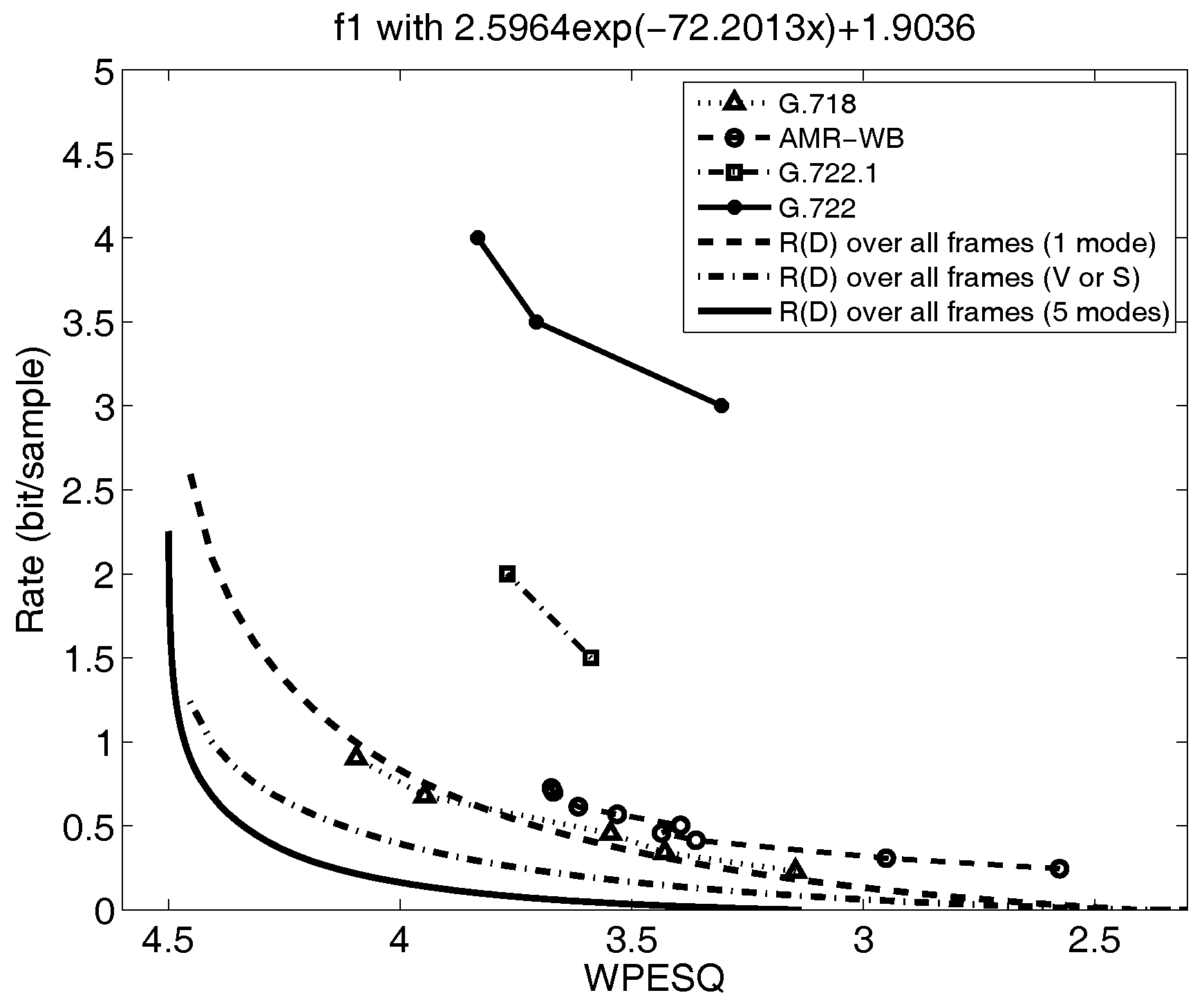
Figure 3 shows three rate distortion functions corresponding to three different models fitted to the same speech utterance. The models range from a single AR(16) or order linear prediction model averaged over all frames (dashed curve), to a two mode (Voiced or Silence) composite source model, where all non-silence frames are fit with one average AR(16) model (dot-dash curve), and a five mode composite source model as shown in Table 1 (solid curve). Note that the mean squared error distortion has been mapped to the WPESQ-MOS [12], where a WPESQ score of 4.0 is considered excellent quality and a WPESQ socre of 3.5 is considered very good. The development of the mapping function is quite complex and outside of the scope of this paper, so we leave those details to the references [8]. We see that the based on the five mode model lower bounds the performance of all of the voice codecs shown in the figure. We also see that the rate distortion function becomes more optimistic about the rate required to achieve a given distortion as the model is made more accurate. The curves shown in Figure 3 emphatically illustrate the dependence of the rate distortion function on the source model, namely, that changes if the source model is changed. The challenge in developing and interpreting rate distortion functions for real-world sources thus involves building and evaluating new source models. As is discussed later in Section 11, this process can naturally lead to new codec designs.
In our following analyses, we utilize the five mode speech model in Table 1. Therefore, we see that the number of subsources or modes is for our models here and the subsources will switch every or more samples (since the frame sizes for speech codecs are at least this large). As a result, the rightmost term in Equation (18) is less than 0.03 bits/sample.
Shown in Figure 4 and Figure 5 are the reverse water filling rate distortion functions for the five mode model from prior work in [8,48], indicated by the dotted lines. Also plotted on the figures are the performance of selected voice codecs from the experiments in the references [8,48]. These rate distortion curves are generated by calculating the conditional for each subsource and then combining these curves at points of equal distortion for all D using the reverse water-filling result in Section 4.2. For Gaussian AR sources, this is equivalent to evaluating the autoregressive expression for the rate distortion function in Section 4.3 parametrically as is varied for each subsource and then combining these at points of equal slope. This requires considerable effort and becomes more unwieldy as the number of subsources increases.
Therefore, it is of interest to evaluate the effectiveness of the several lower bounds mentioned. One explicit lower bound is the small distortion lower bound in Equation (9) from the reverse water-filling section. In this case, the small distortion expression Equation (9) is calculated for all distortions for each subsource and then the ’s are combined at points of equal slope to obtain the for each value of the average distortion. As before, this is equivalent to finding the for each subsource from Equation (13) and combining them. For Gaussian AR sources, this bound on the rate distortion function agrees with the AR lower bound and the Wyner–Ziv lower bound. Gray [29] discusses the relationships among the AR lower bound, the Shannon lower bound, and the Wyner–Ziv lower bound in more detail.
The resulting new, small-distortion lower bounds are denoted by the dark, solid line in Figure 4 and Figure 5. The small distortion lower bound deviates only slightly from the full curve in Figure 4 over the range of distortions of interest, namely WPESQ-MOS from 3.5 to 4.0, but in Figure 5, the new small-distortion lower bound falls away very quickly from the computed by parametric reverse water filling as the WPESQ-MOS drops below 4.0. Thus, the small-distortion lower bound shown in Figure 5 would be far too optimistic concerning the possible performance obtainable by any codec design, and therefore not sufficient as a stand-alone tool to guide speech codec research.
11. R(D) and Codec Design
We have given a general approach to calculating rate distortion functions for real-world sources such as voice and video. Not surprisingly, the method starts with finding a source model and a suitable distortion measure. To obtain a good source model, we have shown that building a composite source model for each sequence is extremely effective since even complex sources can be suitably decomposed into several subsources. Then, we use conditional rate distortion theory to generate the corresponding rate distortion function or a conditional lower bound to the rate distortion function. The resulting is the OPTA for the designed composite source and the specified distortion measure. We have seen how the rate distortion function changes as the source model changes and therefore, the calculation of a rate distortion function that can be used as the OPTA for a real world source consists of devising a good composite source model.
11.1. for Real-World Sources
Revisiting Figure 2, we see that the HEVC video codec has operational rate distortion performance that is closer to the lower bound than the prior H.264 standard. It can be expected that future video codecs will have an operational rate distortion performance that is even better. Will there come a point where the operational rate distortion performance of a video codec gets close to or falls below that of the rate distortion function in Figure 2 as H.264 and HEVC do for the curve without texture information? This cannot be known at this time, but it is clearly possible and even likely. This may be a confusing statement, because, “Don’t rate distortion functions lower bound the best performance of any codec?” Of course, as we have been emphasizing, the functions that we obtain for video or speech are the best performance attainable for the source models that have been calculated from the real-world sources. Real-world sources almost certainly cannot be modeled exactly, so we must settle for the best that we can do; namely, develop the best composite source model that we can and use that model in the calculation of an . We understand that the source model may be improved with later work, and if so, as a result, the rate distortion function will change. As long as we are aware of this underlying dynamic, we have a very effective codec design tool.
11.2. Codec Design Approach
In addition to providing a lower bound to the performance of codecs for real-world sources, such as video and speech, the rate distortion functions can be used to evaluate the performance of possible future new codecs. Here is how. To make the discussion specific, we know that the best performing video codecs that have been standardized, very broadly, perform motion compensated prediction around a discrete transform, possibly combined with intra prediction based on textures within a frame. The H.264 standard has 9 textures for 4 × 4 transform blocks. The composite source model for the calculations of the subsource rate distortion functions shown in Figure 1 use exactly these textures in developing the composite source video model! The composite source model for video used to obtain the in Figure 2 also has a first order temporal correlation coefficient, , which only depends on the temporal frame difference and not conditioned on the texture. The work in [8,38] did not find an improved temporal correlation model by conditioning on texture. Since the in Figure 2 shows considerable performance improvement available for both H.264 and HEVC, the implication is that somehow these codecs may not be taking sufficient advantage of texture information, particularly in conjunction with the motion compensation reference frame memory.
Note the interaction between the codec design and the calculated for a closely related video model. For example, it would be of interest to calculate a composite source model for the new textures and block sizes available in the HEVC standard. Would it actually fall below the current or be very close? The point being emphasized is that video codecs are based on implied models of the source [5] and calculations of bounds are explicitly based on video source models. Thus, it would appear that if one can discern the new video model underlying a proposed new video codec structure, the rate distortion function for this video model could be calculated. As a result, without implementing a new video codec, it is possible to determine the best performance that a codec based on this model might achieve. Since video codec implementations are complex, and many design tradeoffs have to be made, knowing ahead of time how much performance is attainable is an extraordinary tool. Therefore, rate distortion functions have a role in evaluating future video codec designs, a role which has not been exploited, in addition to providing a lower bound on known codec performance.
Of course, the above statements about and codec design also hold for speech sources. The best known standardized speech codecs rely heavily on the linear prediction model as we have done in developing speech models to calculate rate distortion bounds. Multimodal models have played a major role in speech coding and phonetic classification of the input speech into multiple modes and coding each mode differently has lead to some outstanding voice codec designs [44,45,46,47,49]. However, the specific modes in Table 1 are not reflected in the best known standardized codecs such as AMR (Adaptive Multirate) and EVS (Enhanced Voice Services). Developing source models based on the structure of these codecs would lead to additional rate distortion performance curves that could give great insight into how effective the current implementations are to producing the best possible codec performance.
11.3. Small Distortion Lower Bounds
Given the new small distortion lower bounds on the rate distortion functions for a given source model and distortion measure, it is important to consider their utility for codec performance evaluation. If we denote the new small-distortion lower bounds as and the operational rate distortion curve (the actual rate distortion performance achieved by a voice codec) by , then we know that , where is the rate distortion function calculated from the parametric equations. Thus, it is evident that if we find and it is not far below the performance of the voice codec, namely, , then it is not necessary to perform the much more complicated calculations required to generate . In this case we can conclude that, for that source model, the voice codec being evaluated is already close enough to the best performance achievable that no further work on codec design is necessary.
However, if is relatively far below , we cannot state conclusively from these results alone that further codec design work is not required since we do not know how well approximates in general. For this case, we must take the extra effort to perform the repeated parametric calculations necessary to generate the full rate distortion function and compare to . Both Figure 4 and Figure 5 are examples of where the curves are sufficiently far away from the speech codec performance that it would be necessary to perform the parametric calculations to get the true curve; interestingly, we see that in one figure, Figure 4, the lower bound is close to but in the other figure, Figure 5, the lower bound is not tight. In both cases, however, the full curve indicates that further performance gains are possible with future speech codec research.
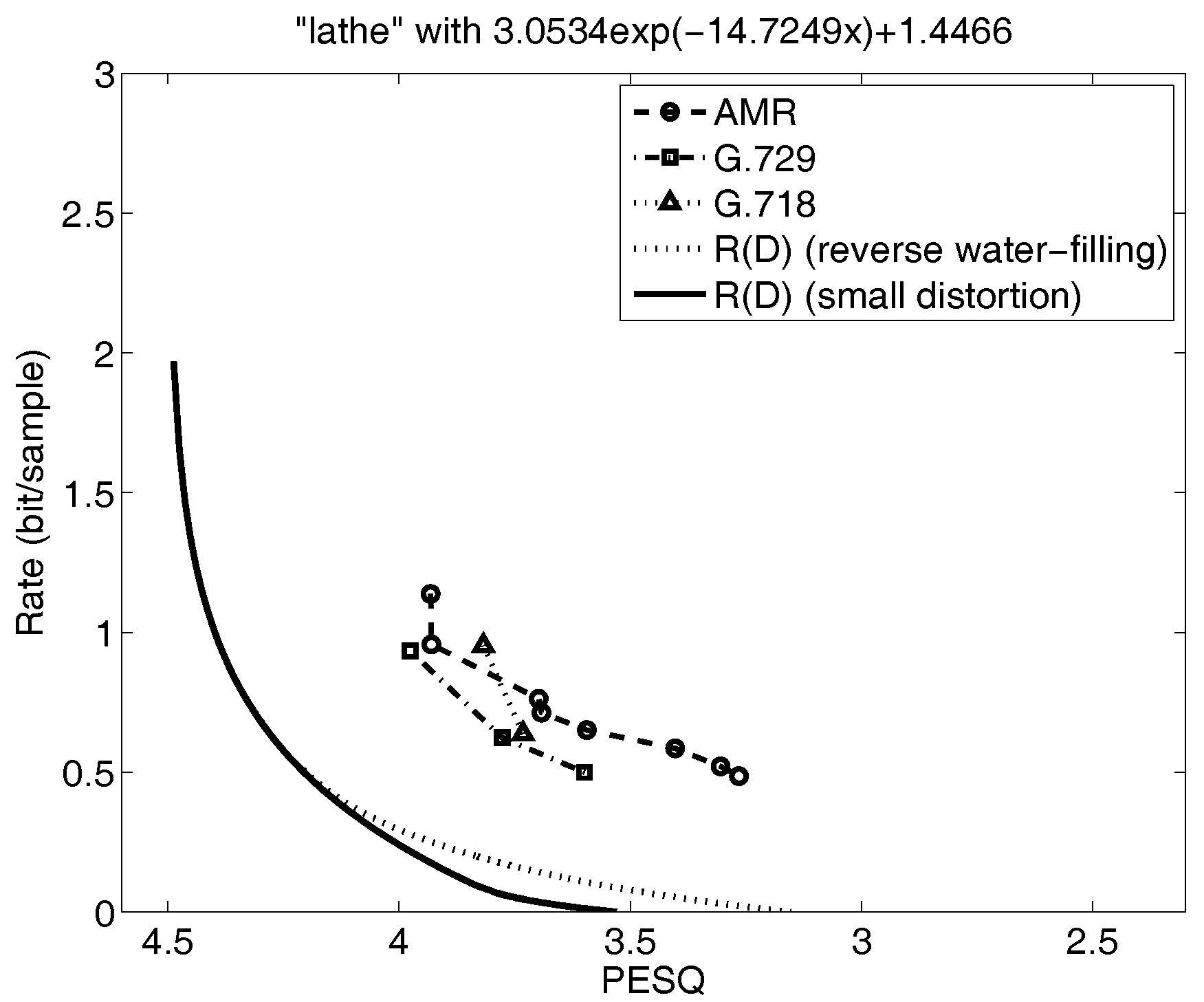
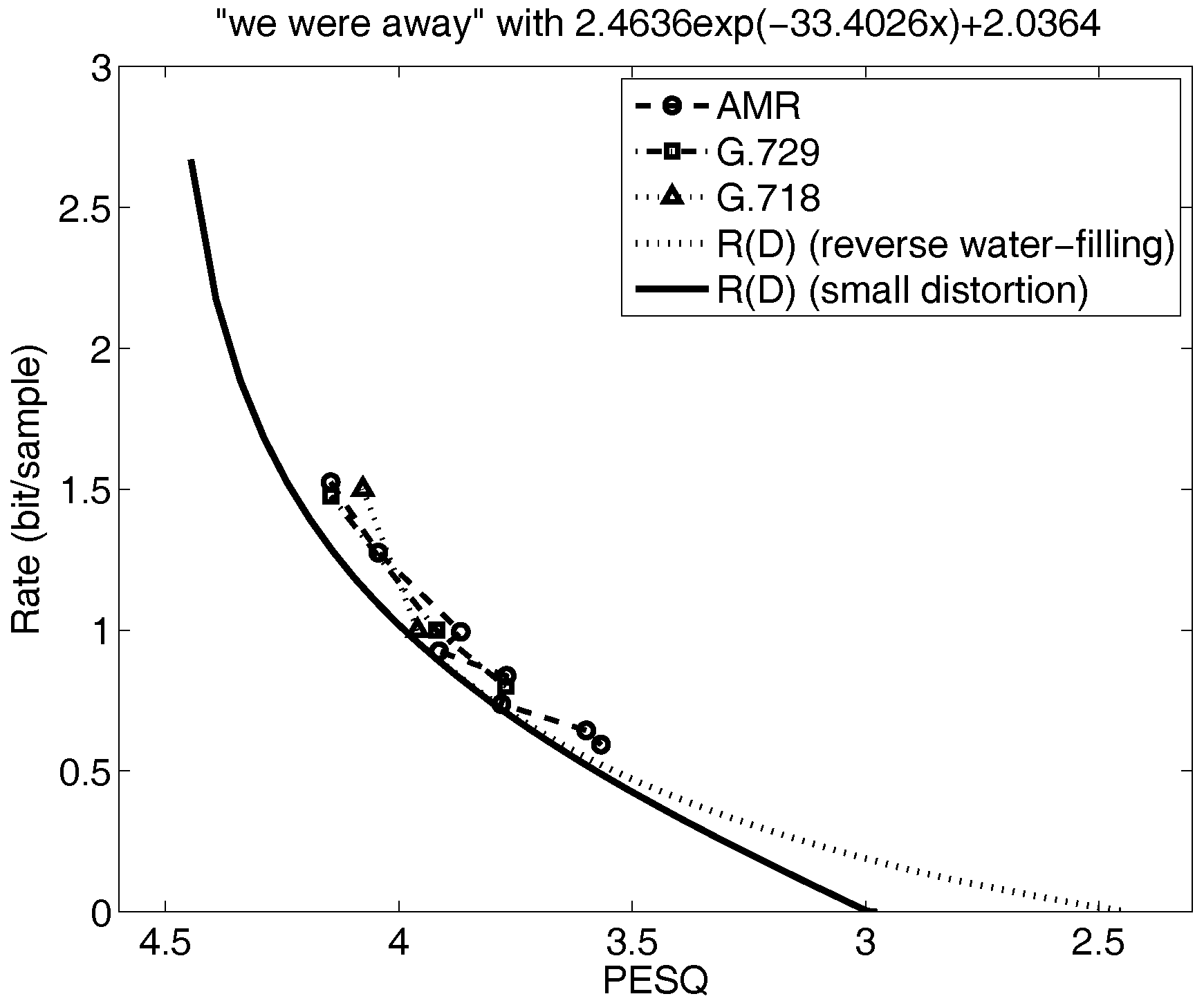
Figure 6 and Figure 7 for narrowband speech illustrate other cases. Specifically, the small distortion lower bound in Figure 6 is far below the speech codec performance so the only way to determine how tight this lower bound is to is to do the parametric calculations for . The result shows that the small distortion lower bound is tight and that more research on optimizing the speech codecs is warranted. On the other hand, the lower bound in Figure 7 is not far below the voice codec performance over the range of distortions of interest and so it would not be necessary to parametrically solve for . And, in fact, when we do, we see that as expected the small distortion lower bound closely approximates for the range of distortions of interest.
Since is much easier to calculate than and can often yield a useful conclusion, the calculation of is a recommended first step in evaluating the performance of existing voice codecs.
12. Conclusions
Rate distortion functions for real-world sources and practical distortion measures can be obtained by exploiting known rate distortion theory results for the MSE distortion measure by creating per realization, composite source models for the sources of interest. A mapping procedure for the distortion measure may be necessary to obtain a perceptually meaningful rate distortion bound. These rate distortion functions provide the optimal performance theoretically attainable for that particular model of the source and the chosen distortion measure. There is a natural interaction between source models for rate distortion calculations and the structure of codecs for real-world sources. This relationship can be exploited to find good codec designs based on the source models used to develop new rate distortion functions, and the source models underlying the best performing codecs can be used to develop new rate distortion bounds. Small distortion lower bounds to rate distortion functions can be useful for initial, easy-to-calculate estimates of the best performance attainable, but must be used carefully in order to avoid overly optimistic performance expectations.
Acknowledgments
Conflicts of Interest
The author declares no conflict of interest.
References
- Shannon, C.E. A mathematical theory of communication. Bell Syst. Tech. J. 1948, 27, 379–423. [Google Scholar] [CrossRef]
- Shannon, C.E. Coding Theorems for a Discrete Source with a Fidelity Criterion. IRE Conv. Rec. 1959, 7, 142–163. [Google Scholar]
- Gallager, R.G. Information Theory and Reliable Communication; John Wiley & Sons, Inc.: New York, NY, USA, 1968. [Google Scholar]
- Netravali, A.N.; Haskell, B.G. Digital Pictures: Representation and Compression; Plenum Press: New York, NY, USA, 1988. [Google Scholar]
- Ortega, A.; Ramchandran, K. Rate-distortion methods for image and video compression. IEEE Signal Process. Mag. 1998, 15, 23–50. [Google Scholar] [CrossRef]
- Effros, M. Optimal Modeling for Complex System Design: The Lessons of Rate Distortion Theory. IEEE Signal Process. Mag. 1998, 15, 51–73. [Google Scholar] [CrossRef]
- Gray, R.M. Conditional Rate-Distortion Theory; Technical Report 6502-2; Stanford Electron. Lab.: Stanford, CA, USA, 1972. [Google Scholar]
- Gibson, J.D.; Hu, J. Rate distortion bounds for voice and video. Found. Trends Commun. Inf. Theory 2014, 10, 379–514. [Google Scholar] [CrossRef]
- Sze, V.; Budagavi, M.; Sullivan, G.J. High efficiency video coding (HEVC). In Integrated Circuit and Systems, Algorithms and Architectures; Springer: New York, NY, USA, 2014; pp. 1–375. [Google Scholar]
- Berger, T. Rate Distortion Theory; Prentice-Hall: Upper Saddle River, NJ, USA, 1971. [Google Scholar]
- ITU-T Recommendation P.862. Perceptual Evaluation of Speech Quality (PESQ), An Objective Method for End-to-End Speech Quality Assessment of Narrow-Band Telephone Networks and Speech Codecs. 2001. Available online: https://www.itu.int/rec/T-REC-P.862 (accessed on 8 November 2017).
- ITU-T Recommendation P.862.2. Wideband Extension to Recommendation P.862 for the Assessment of Wideband Telephone Networks and Speech Codecs. 2007. Available online: https://www.itu.int/rec/T-REC-P.862.2-200511-S/en (accessed on 8 November 2017).
- Cover, T.M.; Thomas, J.A. Elements of Information Theory; Wiley-Interscience: Hoboken, NJ, USA, 2006. [Google Scholar]
- Gray, R.M.; Davisson, L.D. A Mathematical Theory of Data Compression? In Proceedings of the International Conference on Communications, 1974; pp. 40A-1–40A-5. [Google Scholar]
- Gray, R.M. Source Coding Theory; Springer: New York, NY, USA, 1990. [Google Scholar]
- Girod, B. The efficiency of motion-compensating prediction for hybrid coding of video sequences. IEEE J. Sel. Areas Commun. 1987, 5, 1140–1154. [Google Scholar] [CrossRef]
- Flierl, M.; Girod, B. Multiview Video Compression. IEEE Signal Process. Mag. 2007, 24, 66–76. [Google Scholar] [CrossRef]
- Flierl, M.; Mavlankar, A.; Girod, B. Motion and Disparity Compensated Coding for Multiview Video. IEEE Trans. Circuits Syst. Video Technol. 2007, 17, 1474–1484. [Google Scholar] [CrossRef]
- Kalveram, H.; Meissner, P. Rate Distortion Bounds for Speech Waveforms based on Itakura–Saito-Segmentation. Signal Process. IV Theor. Appl. EURASIP. 1988. [Google Scholar]
- Kalveram, H.; Meissner, P. Itakura–Saito clustering and rate distortion functions for a composite source model of speech. Signal Process. 1989, 18, 195–216. [Google Scholar] [CrossRef]
- Gray, R.M. Information rates of autoregressive processes. IEEE Trans. Inf. Theory 1970, 16, 412–421. [Google Scholar] [CrossRef]
- Fontana, R. A Class of Composite Sources and Their Ergodic and Information Theoretic Properties. Ph.D. Thesis, Standford University, Standford, CA, USA, 1978. [Google Scholar]
- Garde, S. Communication of Composite Sources. Ph.D. Thesis, Univeristy of California, Berkeley, CA, USA, 1980. [Google Scholar]
- Naraghi-Pour, M.; Hegde, M.; Arora, N. DPCM encoding of regenerative composite processes. IEEE Trans. Inf. Theory 1994, 40, 153–160. [Google Scholar] [CrossRef]
- Carter, M. Source Coding of Composite Sources. Ph.D. Thesis, The University of Michigan, Ann Arbor, MI, USA, 1984. [Google Scholar]
- Tziritas, G. Rate distortion theory for image and video coding. In Proceedings of the International Conference on Digital Signal Processing, Limassol, Cyprus, 26–28 June 1995. [Google Scholar]
- Mitrakos, D.; Constantinides, A. Maximum likelihood estimation of composite source models for image coding. In Proceedings of the IEEE International Conference on Acoustics, Speech and Signal Processing, Boston, MA, USA, 14–16 April 1983; Volume 8, pp. 1244–1247. [Google Scholar]
- Gibson, J.D.; Hu, J.; Ramadas, P. New Rate Distortion Bounds for Speech Coding Based on Composite Source Models. In Proceedings of the Information Theory and Applications Workshop (ITA), San Diego, CA, USA, 31 January–5 February 2010. [Google Scholar]
- Gray, R.M. A new class of lower bounds to information rates of stationary sources via conditional rate-distortion functions. IEEE Trans. Inf. Theory 1973, 19, 480–489. [Google Scholar] [CrossRef]
- Wyner, A.D.; Ziv, J. Bounds on the Rate-Distortion Function for Stationary Sources with Memory. IEEE Trans. Inf. Theory 1971, 17, 508–513. [Google Scholar] [CrossRef]
- Grenander, U.; Rosenblatt, M. Statistical Analysis of Stationary Time Series; Wiley: New York, NY, USA, 1957. [Google Scholar]
- Hu, J.; Gibson, J.D. Rate distortion bounds for blocking and intra-frame prediction in videos. In Proceedings of the Information Theory and Applications Workshop, University of California, San Diego, CA, USA, 8–13 February 2009. [Google Scholar]
- Habibi, A.; Wintz, P.A. Image coding by linear transformation and block quantization. IEEE Trans. Commun. Technol. 1971, 19, 50–62. [Google Scholar] [CrossRef]
- O’Neal, J.B., Jr.; Natarajan, T.R. Coding isotropic images. IEEE Trans. Inf. Theory 1977, 23, 697–707. [Google Scholar] [CrossRef]
- Clarke, R.J. Transform Coding of Images; Academic Press: London, UK, 1985. [Google Scholar]
- Tasto, M.; Wintz, P.A. A bound on the rate-distortion function and application to images. IEEE Trans. Inf. Theory 1972, 18, 150–159. [Google Scholar]
- Hu, J.; Gibson, J.D. New Rate Distortion Bounds for Natural Videos Based on a Texture-Dependent Correlation Model. IEEE Trans. Circuits Syst. Video Technol. 2009, 19, 1081–1094. [Google Scholar]
- Hu, J.; Gibson, J.D. New rate distortion bounds for natural videos based on a texture dependent correlation model in the spatial-temporal domain. In Proceedings of the 46th Annual Allerton Conference on Communication, Controls, and Computing, Urbana-Champaign, IL, USA, 23–26 September 2008. [Google Scholar]
- Hu, J.; Gibson, J.D. New rate distortion bounds for natural videos based on a texture dependent correlation model. In Proceedings of the IEEE international Symposium on Information Theory, Nice, France, 24–29 June 2007. [Google Scholar]
- Hu, J.; Gibson, J.D. New Block-Based Local-Texture-Dependent Correlation Model of Digitized Natural Video. In Proceedings of the 40th Annual Asilomar Conference on Signals, Systems and Computers, Pacific Grove, CA, USA, 29 October–1 November 2006. [Google Scholar]
- Bross, B.; Han, W.J.; Ohm, J.R.; Sullivan, G.J.; Wiegand, T. High Efficiency Video Coding (HEVC) text specification draft 9 (JCTVC-K1003 v10). 2012. [Google Scholar]
- Gibson, J.D.; Berger, T.; Lookabaugh, T.; Lindbergh, D.; Baker, R.L. Digital Compression for Multimedia: Principles and Standards; Morgan Kaufmann Publishers Inc.: San Francisco, CA, USA, 1998. [Google Scholar]
- Gibson, J.D. Speech Compression. Information 2016, 7, 32. [Google Scholar] [CrossRef]
- Wang, S.; Gersho, A. Phonetically-based vector excitation coding of speech at 3.6 kbit/s. In Proceedings of the 1989 International Conference on Acoustics, Speech, and Signal Processing, ICASSP-89, Glasgow, UK, 23–26 May 1989; pp. 49–52. [Google Scholar]
- Wang, S.; Gersho, A. Improved Phonetically-Segmented Vector Excitation Coding at 3.4 Kb/s. In Proceedings of the 1992 IEEE International Conference on Acoustics, Speech, and Signal Processing (ICASSP-92), San Francisco, CA, USA, 23–26 March 1992. [Google Scholar]
- Das, A.; Gersho, A. A variable-rate natural-quality parametric speech coder. In Proceedings of the IEEE International Conference on Communications, SUPERCOMM/ICC’94, Conference Record, Serving Humanity Through Communications, New Orleans, LA, USA, 1–5 May 1994; Volume 1, pp. 216–220. [Google Scholar]
- Das, A.; Paksoy, E.; Gersho, A. Multimode and Variable-Rate Coding of Speech. In Speech Coding and Synthesis; Kleijn, W., Paliwal, K., Eds.; Elsevier Science: New York, NY, USA, 1995; pp. 257–288. [Google Scholar]
- Gibson, J.D.; Li, Y.Y. Rate Distortion Performance Bounds for Wideband Speech. In Proceedings of the Information Theory and Applications Workshop (ITA), San Diego, CA, USA, 5–10 February 2012. [Google Scholar]
- Atal, B.S.; Hanauer, S.L. Speech analysis and synthesis by linear prediction of the speech wave. J. Acoust. Soc. Am. 1971, 50, 637–655. [Google Scholar] [CrossRef] [PubMed]
Figure 1.
Marginal rate distortion functions for different local textures, , for a frame in paris.cif (from [8]).
Figure 1.
Marginal rate distortion functions for different local textures, , for a frame in paris.cif (from [8]).

Figure 2.
Comparison of rate distortion bounds and the operational rate distortion curves of AVC/H.246 and HEVC for inter-frame coding for the first 5 frames of paris.cif (from [8]).
Figure 2.
Comparison of rate distortion bounds and the operational rate distortion curves of AVC/H.246 and HEVC for inter-frame coding for the first 5 frames of paris.cif (from [8]).

Figure 3.
The rate distortion bounds and the operational rate distortion performance of wideband speech F1 using WPESQ as the distortion measure. The MSE rate distortion bound is mapped to WPESQ as the distortion measure by using the mapping function (13 pairs) (from [8,48]).

Figure 4.
The rate distortion bounds, operational rate distortion performance of speech codecs, and small distortion lower bound for the wideband sequence F1 (adapted from [8,48]).
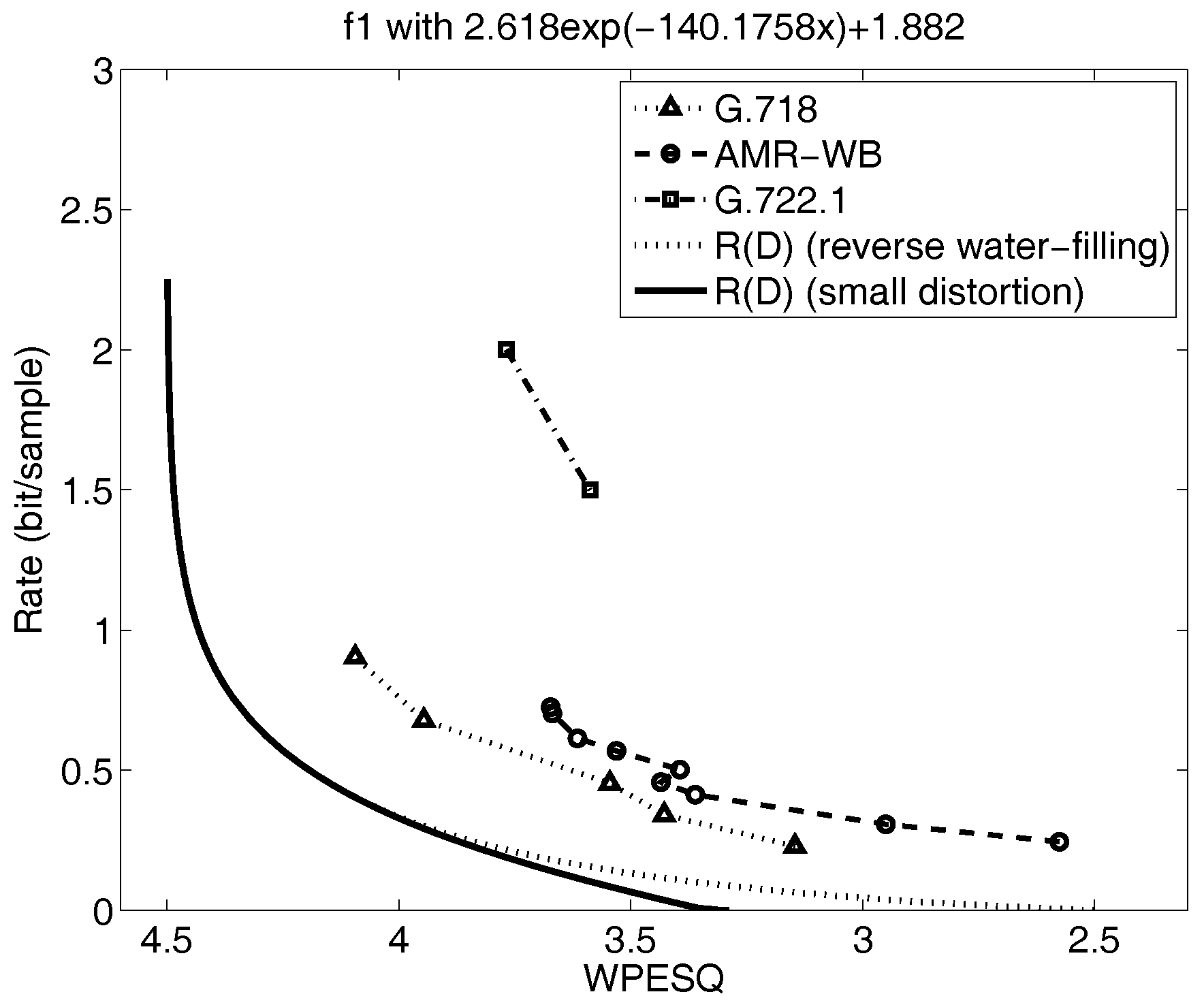
Figure 5.
The rate distortion bounds, operational rate distortion performance of speech codecs, and the small distortion lower bound for the wideband sequence M3 (adapted from [8,48]).
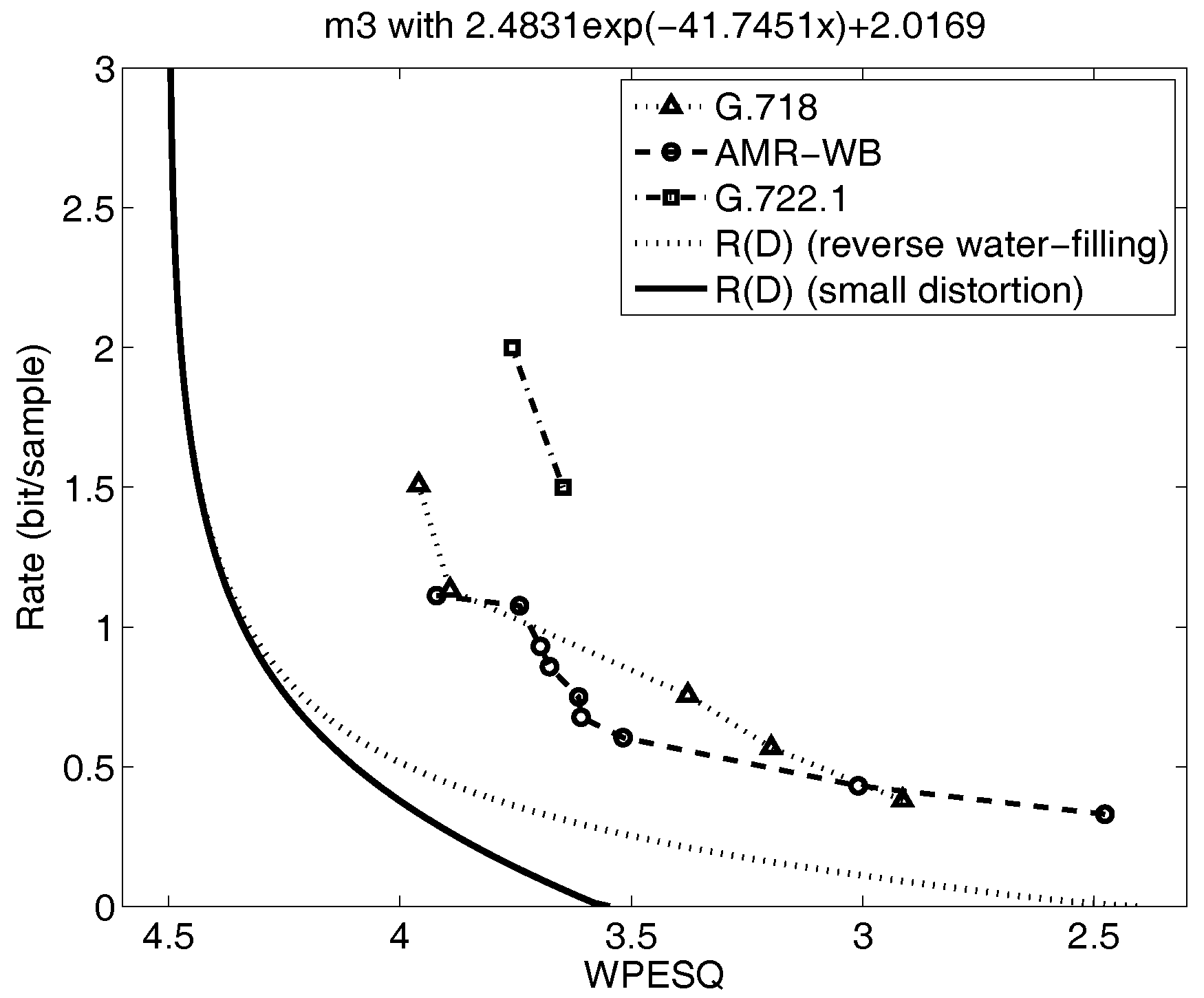
Figure 6.
The rate distortion bounds, operational rate distortion performance of speech codecs, and small distortion lower bound for the narrowband sequence “A lathe is a big tool.” (adapted from [8]).
Figure 6.
The rate distortion bounds, operational rate distortion performance of speech codecs, and small distortion lower bound for the narrowband sequence “A lathe is a big tool.” (adapted from [8]).

Figure 7.
The rate distortion bounds, operational rate distortion performance of speech codecs, and small distortion lower bound for the narrowband sequence “We were away a year ago.”(adapted from [8].
Figure 7.
The rate distortion bounds, operational rate distortion performance of speech codecs, and small distortion lower bound for the narrowband sequence “We were away a year ago.”(adapted from [8].


Table 1.
Composite Source Models for Wideband Speech Sentences (from [48]).
Table 1.
Composite Source Models for Wideband Speech Sentences (from [48]).
| Sequence | Mode | Autocorrelation Coefficients for V, ON, H Average Frame Energy for UV | Mean Square Prediction Error | Probability |
|---|---|---|---|---|
| F1 (Female) (active speech level: dBov) (sampling rate: 12.8 kHz) | V | [1 ] | ||
| ON | [1 ] | |||
| H | 0 | |||
| UV | ||||
| S | ||||
| M3 (Male) (active speech level: dBov) (sampling rate: 12.8 kHz) | V | [1 ] | ||
| ON | [1 ] | |||
| H | [1 ] | |||
| UV | ||||
| S |
© 2017 by the author. Licensee MDPI, Basel, Switzerland. This article is an open access article distributed under the terms and conditions of the Creative Commons Attribution (CC BY) license (http://creativecommons.org/licenses/by/4.0/).
Share and Cite
MDPI and ACS Style
Gibson, J. Rate Distortion Functions and Rate Distortion Function Lower Bounds for Real-World Sources. Entropy 2017, 19, 604. https://doi.org/10.3390/e19110604
AMA Style
Gibson J. Rate Distortion Functions and Rate Distortion Function Lower Bounds for Real-World Sources. Entropy. 2017; 19(11):604. https://doi.org/10.3390/e19110604
Chicago/Turabian StyleGibson, Jerry. 2017. "Rate Distortion Functions and Rate Distortion Function Lower Bounds for Real-World Sources" Entropy 19, no. 11: 604. https://doi.org/10.3390/e19110604
Note that from the first issue of 2016, this journal uses article numbers instead of page numbers. See further details here.