A New Stochastic Dominance Degree Based on Almost Stochastic Dominance and Its Application in Decision Making


1
School of Economics and Management, North China Electric Power University, Beijing 102206, China
2
Beijing Key Laboratory of New Energy and Low-Carbon Development, North China Electric Power University, Changping, Beijing 102206, China
3
China Development Bank, Guizhou Branch, Guizhou 550000, China
*
Author to whom correspondence should be addressed.
Entropy 2017, 19(11), 606; https://doi.org/10.3390/e19110606
Submission received: 11 September 2017
/
Revised: 6 November 2017
/
Accepted: 12 November 2017
/
Published: 17 November 2017
(This article belongs to the Section Information Theory, Probability and Statistics)
Abstract
:Traditional stochastic dominance rules are so strict and qualitative conditions that generally a stochastic dominance relation between two alternatives does not exist. To solve the problem, we firstly supplement the definitions of almost stochastic dominance (ASD). Then, we propose a new definition of stochastic dominance degree (SDD) that is based on the idea of ASD. The new definition takes both the objective mean and stakeholders’ subjective preference into account, and can measure both standard and almost stochastic dominance degree. The new definition contains four kinds of SDD corresponding to different stakeholders (rational investors, risk averters, risk seekers, and prospect investors). The operator in the definition can also be changed to fit in with different circumstances. On the basis of the new SDD definition, we present a method to solve stochastic multiple criteria decision-making problem. The numerical experiment shows that the new method could produce a more accurate result according to the utility situations of stakeholders. Moreover, even when it is difficult to elicit the group utility distribution of stakeholders, or when the group utility distribution is ambiguous, the method can still rank alternatives.
1. Introduction
In some real-life decision situations, such as some public projects, decision makers (DMs) are just agents of all stakeholders. The decision should be made based on the preference of all stakeholders, but not the agents’. In such cases, the elicitation of a unique probability or utility function may be difficult and its use is questionable [1]. One well-regarded method for comparing two alternatives with uncertain utility information is via the idea of stochastic dominance (SD). SD is based on the comparison of the distribution functions that are associated to the alternatives, and can be given the following interpretation: means that the choice of over is rational, in the sense that we prefer the alternative with a greater probability of providing a utility above a certain threshold , and this for all possible [2]. SD rules are widely used to identify SD relations for pairwise comparisons of alternatives under uncertain environment [3,4]. They are robust analytical tools for solving decision making problems under uncertainty [1,5], and have been applied in economics and finance [6,7] because of less restrictive assumptions.
As one method for comparing two alternatives with uncertain information, SD rules have many advantages. It takes the difference of stakeholders’ utility function into account and compares the expected utility of alternatives pairwise, only makes the minimal assumption about the utility function, and makes no assumptions at all with respect to the particular probability distributions of returns [8,9]. However, the disadvantages of this method are also obvious. Firstly, SD rules are often too strong [10], where “strong” means that the stochastic dominance rules are too strict to satisfy. So, normally it is difficult to obtain dominance relationships for all pairwise alternatives. Leshno and Levy [11] noticed that such strict rules relate to “all” utility functions in a given class, including extreme ones that presumably rarely represents stakeholders’ preference. They proved that SD rules may fail to show dominance in cases where almost everyone would prefer one gamble to another. Secondly, SD relations are qualitative rather than quantitative. Here, “qualitative” indicates that the stochastic dominance rules can only be used to judge whether there is a dominance relation among pairwise alternatives, but fail to measure the degree of this dominance relation. Only ordinal concepts are involved and the degree that one alternative dominates another is unknown, although the SD relation is determined. Nowak [12] believed that it is not reasonable to accept strict preference if the alternatives differ insignificantly. The strict preference that is based on SD rules is groundless in many situations and may cause problems in decision aid. He argued that the verification of SD relations is not sufficient to accept strict preference. To better apply the SD rules, the method to measure the stochastic dominance degree (SDD) is necessary [13].
To solve these problems, scholars have made many attempts. One possible solution is the relaxation of SD rules. Leshno and Levy [11] defined the concept of almost stochastic dominance (ASD). It is a form of SD that holds for most, but not all, of the utility functions in a given class. Some utility functions are deemed “extreme”, and it is assumed that they do not represent the preferences of any real-world stakeholder. They suggested that such utility functions should be ruled out. On the other hand, some scholars paid their attention to the issue regarding the quantification of SD rules. Several studies testing for SD have been carried out [14,15,16] based on different SDD definitions. Some SDD definitions have been proposed [17,18,19]. For example, Zhang, Fan and Liu [17] introduced a concept of stochastic dominance degree to describe the extent to which one alternative dominates another when the SD relation for each pair of alternatives is determined, and a computation formula of the SDD is given.
In this paper, we firstly review the existing SD and ASD rules, and supplement the definitions of ASD (Section 2). Then, we propose a new SDD definition based on the idea of ASD (Section 3). The new definition contains four kinds of SDDs corresponding to four risk preference styles. It can measure the degree of SD and ASD, and has clear economic meaning. For an alternative, its SDD is determined by its own performance and the support from the stakeholders, and varies with the utility situations of stakeholder group. Furthermore, a SDD based method is proposed to solve stochastic multiple criteria decision making (MCDM) problems (Section 4). Next, a numerical example and comparative analysis are showed in Section 5. Finally, the paper is concluded in Section 6.
2. Stochastic Dominance and Almost Stochastic Dominance
In this section we briefly review the various SD rules analyzed in this paper. Then, following Levy’s [20] and Tzeng’s [21] definitions of almost first degree stochastic dominance (AFSD) and almost second degree stochastic dominance (ASSD), we further supplement the definitions of almost second degree inverse stochastic dominance (ASISD), and almost prospect stochastic dominance (APSD).
2.1. Stochastic Dominance
Let us first define several sets of utility functions corresponding to the various SD rules following Levy and Wiener [22]. In each case we assume the utility function to be continuous and piecewise smooth.
- is the set of increasing utility functions (rational investors). is equivalent to for all .
- is the set of increasing and concave utility functions (risk averters). is equivalent to and for all .
- is the set of increasing and convex utility functions (risk seekers). is equivalent to and for all .
- is the set of all S-shaped utility functions as suggested by Prospect Theory (prospect investors). is equivalent to for all , and for all , and for all . This means risk seeking for losses and risk aversion for gains.
Definition 1
[17,23]. Let and be two random variables, and be the cumulative distribution functions of and , respectively, be the finite support of cumulative distributions, where and are the most extreme limits on our distributions of returns. Let and be the two expectations, respectively. Let FSD, SSD, SISD and PSD denote first degree, second degree, second degree inverse and prospect stochastic dominance, respectively. The SD rules are:
- (1)
- if and only if
- (i)
- for all with strict inequality for some , or
- (ii)
- for all with strict inequality for some ;
- (2)
- if and only if
- (i)
- for all with strict inequality for some , or
- (ii)
- for all with strict inequality for some ;
- (3)
- if and only if
- (i)
- for all with strict inequality for some , or
- (ii)
- for all with strict inequality for some ;
- (4)
- if and only if
- (i)
- for all with strict inequality for some , or
- (ii)
- for all and with strict inequality for some and .
There are in turn higher orders of SD, which might yield conclusive results when FSD, SSD, SISD, and PSD do not. They were considered too complex for practical use and calculation. We will not pursue them further here.
SD rules have proven extremely useful not only in financial economics and operations research, but in many other areas of science [20,24]. However, SD rules suffer from a serious drawback. SD rules are strong conditions and generally a SD relation between two alternatives does not exist. Such strict rules relate to all utility functions in a given class, including extreme ones, which presumably rarely represents stakeholders’ preference. While “most” stakeholders may prefer one uncertain alternative over another, SD rules will not reveal this preference due to some extreme utility functions in the case of even a very small violation of these rules.
2.2. Almost Stochastic Dominance
The Almost Stochastic Dominance rules have been developed as an extension of the standard SD framework to solve such paradoxes. The core idea of ASD is to relax the strict restrictions on distribution functions by eliminating some extreme utility functions, and to obtain the dominance relation held by almost all stakeholders (those with reasonable preferences). Hence they were named Almost Stochastic Dominance. Leshno and Levy [11] firstly gave the definition of almost first degree stochastic dominance (AFSD) in 2002.
Definition 2
[11]. Let and be two random variables, and be the cumulative distribution functions of and , respectively, be the finite support of cumulative distributions, where and are the most extreme limits on our distributions of returns. For every , define: , almost first degree stochastic dominance ( ), if and only if,
- (i)
- for all , or
- (ii)
- ;
where and .
Note that we replaced original “” with “” in this paper to facilitate next calculation.
Although Leshno and Levy [11] have proposed the definition of almost second-degree stochastic dominance (ASSD) in 2002, Tzeng and Shih [21] as well as Huang et al. [25] proved that Levy’s [11] definition is incorrect and gave the correctional definition of ASSD. Next, we follow Tzeng’s [21] definition and further provide the definitions of ASISD and APSD.
First, let us define the sets of , , and as:
where and ; and .
The sets of almost utility functions are defined as:
where , .
Tzeng’s ASSD was defined as follow:
Definition 3
- (i)
- for all , or
- (ii)
- and ;
where .
Similarly, we define ASISD as follows.
Definition 4.
For every , almost second degree inverse stochastic dominance (), if and only if,
- (i)
- for all , or
- (ii)
- and ;
where .
Based on above definition, we propose the definition of APSD:
Definition 5.
For every , almost prospect stochastic dominance (), if and only if,
- (i)
- for all , or
- (ii)
- , and ;
where , .
In these definitions, the role of is such that, when it takes values closer to 1, the ASD relation does not to hold for a wider range of distributions of the prospects X and Y. Of course, these distributions are unknown in most practical applications and must be estimated. For a discussion of inference in this case on SD and ASD relations, please refer to Post [14], Post and Potì [15] and Linton et al. [16].
Next, the definitions of SDD will be presented based on the ASD.
3. Stochastic Dominance Degree
According to Definition 2, we state the following proposition:
Proposition 1.
Let , for the stakeholders whose utility function satisfy , it must be that , namely dominate .
The value of reflects the number of people who hold dominate . In practice, the more people support dominate , we should believe better than . Therefore, we choose as an indicator with respect to the dominance degree of alternatives.
On the other hand, mean is a simple and time-honored method taken from financial applications to measure the value of uncertain number. Many methods, such as Mean-variance (MV) and mean-semivariance, regard mean as an important indicator to judge the priority of alternatives [1]. Although the introduction of utility function makes expected utility and mean unequal. There is still positive correlation between them. Especially when some extreme utility functions are excluded, then the correlation increases further. Therefore, we choose the mean as the other indicator. The first degree SDD are defined based on the two aspects.
Definition 6.
If (either almost or standard), then the first degree SDD of (noted as ) is given by
where and , is a function having the following properties:
- (a)
- , if ;
- (b)
- .
The symbol denotes an operator that is used to combine the two indicators, and . It can be multiplication (), exponentiation () or other special rules defined by DMs. Parameters also can be introduced into it to adjust the weights of two indicators. In practice, the function reflects the group utility situation of stakeholders. That is what percentage of stakeholders hold utility function . The given conditions are implied by the SD relations. Note that, when , ASD is reduced to standard SD. .
Following the same argument used for first degree SDD, we obtain the SDD of the others (second degree, second degree inverse and prospect). The universal definition of SDD is shown in the following:
Definition 7.
If (either almost or standard first degree, second degree, second degree inverse and prospect SD), then the SDD of (noted as ) is given by
where , and .
is a function having the following properties:
- (a)
- , if ;
- (b)
- .
When compared with determining every stakeholder’s utility function, constructing a group utility situation function is much easier. Group utility situation is more stable than individual utility [26]. Moreover, due to the monotonicity of function , sometimes, we can obtain the decision results directly, without determining the specific group utility situation function (e.g., following example).
The new SDDs take both objective mean and stakeholders’ subjective preferences into account together. It can measure both SD and ASD degree, and correct for certain conditions where standard SD yields results that are inconsistent with the common-sense preferences of most stakeholders. Next, an example is given to investigate the superiority of the proposed SDDs further.
Suppose that ten experts evaluate three alternatives A1; A2; A3 on a scale of ten (1, the worst; 10, the best), and evaluations of the alternatives are expressed in the form of probability distributions as shown in Table 1. The decision analysis with the proposed SDD is shown as follow.
According to the data in Table 1, the cumulative distribution functions of A1, A2, and A3 are shown in Figure 1. In Figure 1, S1 denotes the area enclosed by the lines for A1 and A2 under the curve for A1, and S2 denotes the area between the curves for A2 and A1 under the curve for A2. According to Definition 6, we can get:
Similarly, the others SDD indicators are computed as shown in Table 2.
From Table 2, we can see that there are only a standard SSD relation and a standard SISD relation between A2 and A3. Obviously, we cannot obtain the dominance relation according to standard SD rules. However, duo to the relaxation of restrictions on distribution functions, the proposed SDD can obtain the dominance relation between alternatives more easily. According to the first degree SDD indicators ( and ) in Table 2, we can confirm , directly. Then, we obtain , since and .
Moreover, the decision results will change with stakeholders’ risk preference styles. This is more reasonable. In Table 2, if we compare A1 with A3 without reference A2, we cannot distinguish the two alternatives by the first degree SDD indicators. This is because the precondition of first degree ASD just claims that is an increasing utility functions set, but does not restrict the risk preference styles of stakeholders. If we know stakeholders’ risk preference styles, we can use corresponding higher degree SDDs (second degree for risk averters, second degree inverse for risk seekers, prospect for prospect investors) to confirm dominance relation more accurately. In the above example, we get , hence risk averters will think . Whereas, for risk seekers, , hence . In practical decision making, the results derived from different SDDs may be inconsistent. DMs should choose one kind of SDDs according to the risk preference styles of stakeholders, rather than use several of them simultaneously. When we just know that all of the stakeholders are rational investors (), we should choose first degree SDD. If we know stakeholders’ risk preference styles, we can use corresponding higher degree SDDs for more precise results.
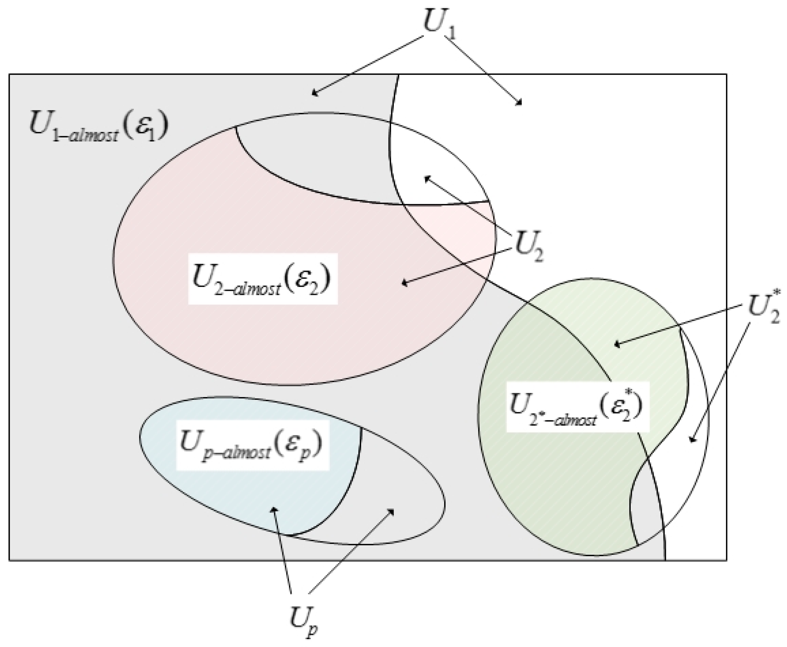
In addition, the new definition has clearing economic meaning and contributes to theory study. The property of hierarchy, i.e., FSD implies SSD, which, in turn, implies that third degree stochastic dominance (TSD) is an important property for SD rules. Guo, et al. [27] found that ASD rules do not possess the property. But they did not explain the reason. Now, with the new SDD definition, we can explain it clearly. That is because in the standard SD, , , and are the subset of . If all rational investors () hold a SD relation (i.e., FSD), all risk averters, risk seekers, and prospect investors (, or ) will hold the same SD relation. However, in ASD, when , , , the sets, , , and , may not be not included in the set (shown in Figure 2). In other words, although all DMs holding support certain dominate relation, some DMs holding , or may still not support that dominate relation.
4. A Method for Stochastic MCDM
Consider a stochastic MCDM problem. Let be a discrete set of alternatives, and be the set of attributes, is the weight vector of the attribute, with and . Usually, the weight vector can be obtained either directly from the DMs or indirectly using existing procedures, such as Analytic Hierarchy Process (AHP) [28]. Suppose that is a decision matrix, where is a random variable with probability distribution function , provided by DMs for the alternative with respect to the attribute . The problem concerned in this paper is to rank alternatives or to select the most desirable alternatives among a finite set based on decision matrix and attribute weight vector .
To solve the stochastic MCDM problem mentioned above, we propose a decision analysis method based on SDD. A description of the method is given below.
- Step 1.
- Identify the SD or ASD relation for pairwise comparisons of alternatives with respect to each attribute, and then calculate the SDD that an alternative dominates another by Definition 7, set up SDD matrix for each attribute, where denote the SDD of alternative dominates with respect to the attribute .
- Step 2.
- According to SDD matrix , calculate relative dominant degree on each attribute with a PROMETHEE-II based method. Then construct relative dominant degree matrix .
- Step 3.
- Normalize the relative dominant degree matrix into .For benefit-type criteria:For cost-type criteria:
- Step 4.
- Calculate overall dominant degree matrix by Equation (5).
- Step 5.
- Determine the ranking result of alternatives according to , .
A brief description of the PROMETHEE-II based method in step 3 is given below.
Let be the dominant degree which is a measure that alternative is dominating the other alternatives on attribute , and be the non-dominant degree, which is a measure that alternative is dominated by the other alternatives on attribute . Here, and can be, respectively, defined by the following formulas:
Let be the relative dominant degree, which measures the difference between dominant and non-dominant degrees of alternative on attribute . can be calculated by the following formula:
5. A Numerical Example
5.1. Illustrative Applications
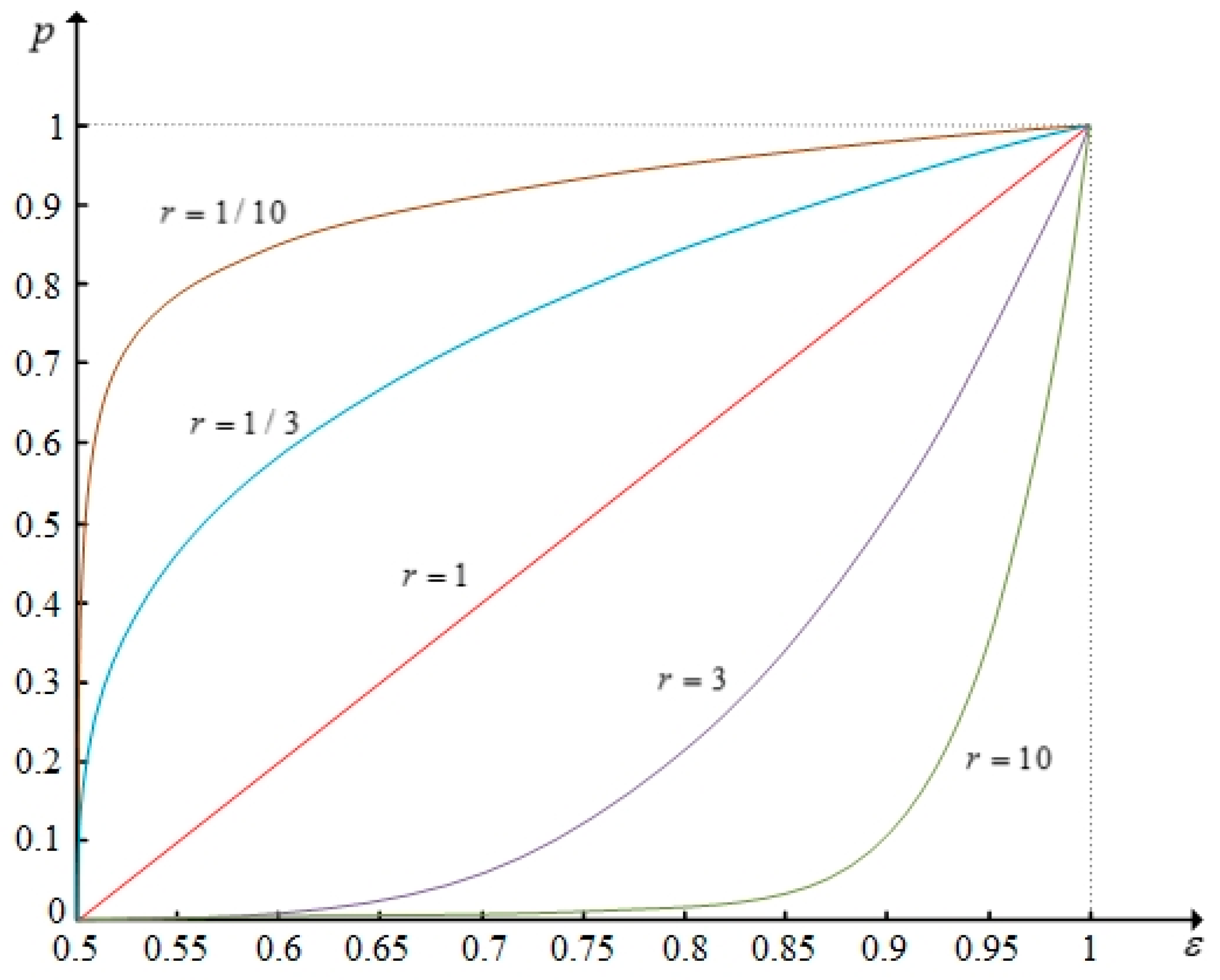
Following Martel and Zaras [29], Nowak [12], and Liu et al. [18], we consider the same problem of selecting the most desirable one from ten computer development projects (A1, A2, ..., A10). The decision-making committee assesses the projects based on four attributes which follow: (1) personal resources effort (C1); (2) discounted profit (C2); (3) chances of success (C3); and, (4) technological orientation (C4). The weight vector of the attribute provided by the DMs is . The evaluation group is constituted by seven experts. The evaluations on the projects with respect to the criteria provided by the evaluation group are expressed in the form of probability distributions, as shown in Table 3. In the example, we assume that is a multiplication operator and the function () (Figure 3).
Firstly, we set and calculate decision results by first degree SDD. Decision steps and some computation results are shown as follows:
Calculate the SDD with Equation (2), set up SDD matrix for each attribute. The SDD matrixes for each attribute are showed as follow:
Construct relative dominant degree matrix with Equations (6)–(8). The relative dominant degree matrix is shown as follows:
Normalize the relative dominant degree matrix with Equations (3) and (4):
Calculate overall dominant degree matrix with Equation (5):
The ranking result of alternatives is .
Similarly, we can obtain the overall dominant degree matrix that is calculated by second degree and second degree inverse SDD as follows:
Suppose that the reference point is 5. We can also get the overall dominant degree matrix calculated by prospect SDD.
5.2. Comparative Analysis and Discussion
The results obtained by different SDD, Zaras and Martel’s method [29], Nowak’s method [12], and Liu and Fan’s method [18] are shown in Table 4. It can be seen from Table 4 that the results obtained by the proposed SDD method and those by the existing methods are slightly different. However, the proposed method and Liu and Fan’s method [18] could produce more accurate results than the others. When comparing with the existing methods, the new method takes the risk preference styles and group utility distribution of stakeholders into account. The results obtained by the new method will vary with the risk preference styles of stakeholders. It makes the new method more reasonable for practical decision making.
To analyze the impact of group utility distribution of stakeholders on the ranking result, we set 1/10, 1/3, 1, 3, and 10, respectively, then calculate and compare the decision results under first degree SDD. The images of function are shown in Figure 3. The results are shown in Table 5 accordingly. From Figure 3 and Table 5 we can see that the differences in ranking results are slight relative to the significant differences in function . This is because is limited to monotonically increasing function. The group utility distribution of stakeholders has a limited influence over the ranking result. Therefore, when the elicitation of group utility distribution of stakeholders is difficult or the group utility distribution is ambiguous, we can still get ranking results by the proposed method.
6. Conclusions
To overcome the defects in traditional SD rules, we firstly supplement the definitions of ASISD and APSD. Then, we propose a new definition of SDD based on the idea of ASD. When comparing with existing definitions, the new definition takes both objective mean and stakeholders’ subjective preference into account. For an alternative, its SDD is determined by two aspects, its own performance and the support from stakeholders, and vary with the utility situations of the stakeholder group. The new definition contains four kinds of SDD, which are corresponding to different risk preference styles, DMs can choose suitable one according to stakeholders’ situations. The operator in the definition also can be changed to fit in with different circumstances. In addition, with the relaxation of restrictions on distribution functions, it is easier to obtain the dominance relation between alternatives, and both SD and ASD degree can be measured by the same equation.
On the basis of the new SDD, we present a method to solve the stochastic MCDM problem. The numerical experiment shows that the new method could produce more accurate results according to the risk preference styles of stakeholders. Moreover, when it is difficult to elicit the group utility distribution of stakeholders or the group utility distribution is ambiguous, the proposed method can still rank alternatives. Unlike most existing methods, the utility situations of stakeholders are adequately considered in the proposed method. It gives DMs one more choice to solve stochastic MCDM problems according to stakeholders’ preferences.
In the future, further researches will helpful for improving the accuracy of the method. The property of hierarchy is an important property for SD rules. However, existing ASD definitions do not possess the property. It will be very interesting to seek new ASD definitions that are possessing the property of hierarchy. The research regarding to the elicitation of stakeholders’ group utility distribution are significant, too. Furthermore, when considering that the relevant distribution is not completely known due to heterogeneous beliefs, subjective distortion, or estimation error, the inferential frameworks based on entropy and similar information-theoretic measures of distances between distribution will be the focus of our future research.
Acknowledgments
This research is supported by the 2017 Special Project of Cultivation and Development of Innovation Base (No. Z171100002217024), the Research Funds of Beijing Social Science (No. 16GLC069), and the Fundamental Research Funds for the Central Universities (No. 2016MS70), (No. 2017XS098), (No. 2017XS099).
Author Contributions
Yunna Wu and Xiaokun Sun mainly studied the proposed method; Hu Xu carried a numerical example and calculated the result, then Hu Xu drafted the paper. Finally, Chuanbo Xu formatted the manuscript for submission.
Conflicts of Interest
The authors declare no conflict of interest.
References
- Yager, R.R.; Alajlan, N. Probability weighted means as surrogates for stochastic dominance in decision making. Knowl. Based Syst. 2014, 66, 92–98. [Google Scholar] [CrossRef]
- Montes, I.; Miranda, E.; Montes, S. Decision making with imprecise probabilities and utilities by means of statistical preference and stochastic dominance. Eur. J. Oper. Res. 2014, 234, 209–220. [Google Scholar] [CrossRef]
- Wu, Y.; Xu, C.; Xu, H. Optimal site selection of tidal power plants using a novel method: A case in China. Energies 2016, 9, 832. [Google Scholar] [CrossRef]
- Wu, Y.; Xu, H.; Xu, C.; Xiao, X. An almost stochastic dominance based method for stochastic multiple attributes decision making. Intell. Decis.Technol. 2017, 11, 1–13. [Google Scholar] [CrossRef]
- Graves, S.B.; Ringuest, J.L. Probabilistic dominance criteria for comparing uncertain alternatives: A tutorial. Omega 2009, 37, 346–357. [Google Scholar] [CrossRef]
- Hodder, J.E.; Jackwerth, J.C.; Kolokolova, O. Improved Portfolio Choice Using Second Order Stochastic Dominance; Social Science Electronic Publishing: Rochester, NY, USA, 2014. [Google Scholar]
- Zagst, R.; Kraus, J. Stochastic dominance of portfolio insurance strategies. Ann. Oper. Res. 2011, 185, 75–103. [Google Scholar] [CrossRef]
- Montes, I.; Miranda, E.; Montes, S. Stochastic dominance with imprecise information. Comput. Stat. Data Anal. 2014, 71, 868–886. [Google Scholar] [CrossRef]
- Stoyanov, S.V.; Rachev, S.T.; Fabozzi, F.J. Metrization of stochastic dominance rules. Int. J. Theor. Appl. Finance 2012, 15, 203–256. [Google Scholar] [CrossRef]
- Wu, Y.; Xu, H.; Xu, C.; Chen, K. Uncertain multi-attributes decision making method based on interval number with probability distribution weighted operators and stochastic dominance degree. Knowl. Based Syst. 2016, 113, 199–209. [Google Scholar] [CrossRef]
- Leshno, M.; Levy, H. Preferred by “all” and preferred by “most” decision makers: Almost stochastic dominance. Manag. Sci. 2002, 48, 1074–1085. [Google Scholar] [CrossRef]
- Nowak, M. Preference and veto thresholds in multicriteria analysis based on stochastic dominance. Eur. J. Oper. Res. 2004, 158, 339–350. [Google Scholar] [CrossRef]
- Shu, M.H.; Wu, H.C. Supplier evaluation and selection based on stochastic dominance: A quality-based approach. Commun. Stat. Theory Methods 2014, 43, 2907–2922. [Google Scholar] [CrossRef]
- Post, T. Critical Values for Almost Stochastic Dominance Based on Relative Risk Aversion; Social Science Electronic Publishing: Rochester, NY, USA, 2015. [Google Scholar]
- Post, T.; Potì, V. Portfolio analysis using stochastic dominance, relative entropy, and empirical likelihood. Manag. Sci. 2017, 63, 153–165. [Google Scholar] [CrossRef]
- Linton, O.; Maasoumi, E.; Whang, Y.J. Consistent testing for stochastic dominance under general sampling schemes. Rev. Econ. Stud. 2005, 72, 735–765. [Google Scholar] [CrossRef]
- Zhang, Y.; Fan, Z.P.; Liu, Y. A method based on stochastic dominance degrees for stochastic multiple criteria decision making. Comput. Ind. Eng. 2010, 58, 544–552. [Google Scholar] [CrossRef]
- Liu, Y.; Fan, Z.P.; Zhang, Y. A method for stochastic multiple criteria decision making based on dominance degrees. Inf. Sci. 2011, 181, 4139–4153. [Google Scholar] [CrossRef]
- Tan, C.; Ip, W.H.; Chen, X. Stochastic multiple criteria decision making with aspiration level based on prospect stochastic dominance. Knowl. Based Syst. 2014, 70, 231–241. [Google Scholar] [CrossRef]
- Levy, H. Stochastic dominance: Investment decision making under uncertainty. In Studies in Risk and Uncertainty; Springer: Berlin/Heidelberg, Germany, 2006; pp. 757–776. [Google Scholar]
- Tzeng, L.Y.; Shih, P.T. Revisiting almost second-degree stochastic dominance. Manag. Sci. 2013, 59, 1250–1254. [Google Scholar] [CrossRef]
- Levy, H.; Wiener, Z. Stochastic dominance and prospect dominance with subjective weighting functions. J. Risk Uncertain. 1998, 16, 147–163. [Google Scholar] [CrossRef]
- Nowak, M. Aspiration level approach in stochastic mcdm problems. Eur. J. Oper. Res. 2007, 177, 1626–1640. [Google Scholar] [CrossRef]
- Blavatskyy, P.R. Probabilistic Choice and Stochastic Dominance; Springer: Berlin/Heidelberg, Germany, 2012; pp. 59–83. [Google Scholar]
- Huang, R.J.; Tsetlin, I.; Tzeng, L.Y.; Winkler, R.L. Generalized Almost Stochastic Dominance; Institute for Operations Research and the Management Sciences (INFORMS): Catonsville, MD, USA, 2015; Volume 63. [Google Scholar]
- Hwang, C.-L.; Lin, M.-J. Group Decision Making under Multiple Criteria: Methods and Applications; Springer Science & Business Media: Berlin, Germany, 2012; Volume 281. [Google Scholar]
- Guo, X.; Zhu, X.; Wong, W.-K.; Zhu, L. A note on almost stochastic dominance. Econ. Lett. 2013, 121, 252–256. [Google Scholar] [CrossRef] [Green Version]
- Jalao, E.R.; Wu, T.; Dan, S. A stochastic ahp decision making methodology for imprecise preferences. Inf. Sci. 2014, 270, 192–203. [Google Scholar] [CrossRef]
- Martel, J.-M.; Zaras, K. Stochastic dominance in multicriterion analysis under risk. Theory Decis. 1995, 39, 31–49. [Google Scholar] [CrossRef]
Figure 1.
Cumulative distribution functions of A1, A2, and A3.
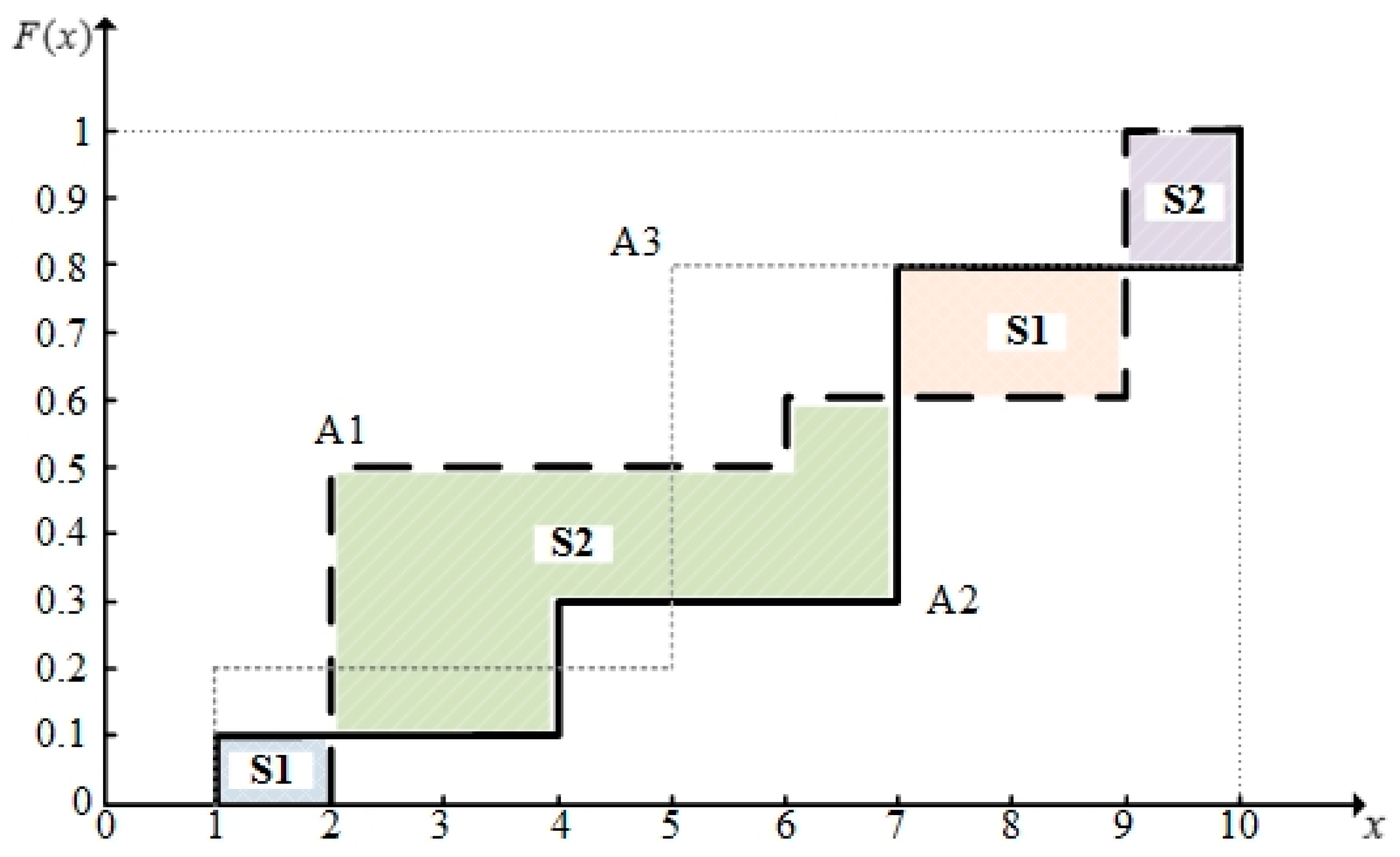
Figure 2.
Relationships among different utility function sets.

Figure 3.
The images of function under different values of .

Table 1.
Distributional evaluations for three alternatives.
| Scores | Alternatives | ||
|---|---|---|---|
| A1 | A2 | A3 | |
| 1 | - | 1/10 | 2/10 |
| 2 | 5/10 | - | - |
| 3 | - | - | - |
| 4 | - | 2/10 | - |
| 5 | - | - | 6/10 |
| 6 | 1/10 | - | - |
| 7 | - | 5/10 | - |
| 8 | - | - | - |
| 9 | 4/10 | - | - |
| 10 | - | 2/10 | 2/10 |
Table 2.
The indicators of stochastic dominance degree (SDD) for three alternatives.
| A1 & A2 | −0.773 | −0.991 | −0.968 | −1.2 |
| A1 & A3 | 0.5 | −0.828 | 0.828 | 0 |
| A2 & A3 | 0.929 | 1 | 1 | 1.2 |
Note: positives mean the former dominate the later; negatives mean the later dominate the former.
Table 3.
Distributional evaluations for the ten projects.
| Criteria | Scores | Alternatives | |||||||||
|---|---|---|---|---|---|---|---|---|---|---|---|
| A1 | A2 | A3 | A4 | A5 | A6 | A7 | A8 | A9 | A10 | ||
| C1 | 1 | 0 | 0 | 0 | 1/7 | 0 | 1/7 | 1/7 | 1/7 | 0 | 0 |
| 2 | 3/7 | 1/7 | 0 | 0 | 0 | 0 | 0 | 2/7 | 0 | 1/7 | |
| 3 | 1/7 | 0 | 0 | 0 | 1/7 | 0 | 0 | 2/7 | 0 | 2/7 | |
| 4 | 0 | 2/7 | 0 | 0 | 0 | 0 | 0 | 1/7 | 0 | 2/7 | |
| 5 | 2/7 | 1/7 | 3/7 | 1/7 | 0 | 0 | 3/7 | 1/7 | 2/7 | 1/7 | |
| 6 | 0 | 2/7 | 1/7 | 0 | 2/7 | 0 | 1/7 | 0 | 1/7 | 0 | |
| 7 | 1/7 | 0 | 1/7 | 0 | 2/7 | 1/7 | 0 | 0 | 3/7 | 1/7 | |
| 8 | 0 | 1/7 | 2/7 | 1/7 | 0 | 3/7 | 1/7 | 0 | 1/7 | 0 | |
| 9 | 0 | 0 | 0 | 4/7 | 2/7 | 0 | 0 | 0 | 0 | 0 | |
| 10 | 0 | 0 | 0 | 0 | 0 | 2/7 | 1/7 | 0 | 0 | 0 | |
| C2 | 1 | 0 | 1/7 | 1/7 | 0 | 0 | 0 | 1/7 | 3/7 | 0 | 0 |
| 2 | 2/7 | 0 | 0 | 0 | 0 | 0 | 3/7 | 3/7 | 0 | 1/7 | |
| 3 | 1/7 | 0 | 0 | 1/7 | 0 | 4/7 | 1/7 | 0 | 1/7 | 0 | |
| 4 | 0 | 0 | 0 | 1/7 | 0 | 0 | 0 | 1/7 | 1/7 | 0 | |
| 5 | 2/7 | 0 | 0 | 0 | 1/7 | 0 | 1/7 | 0 | 0 | 0 | |
| 6 | 0 | 1/7 | 1/7 | 1/7 | 2/7 | 0 | 1/7 | 0 | 1/7 | 0 | |
| 7 | 0 | 1/7 | 0 | 0 | 1/7 | 1/7 | 0 | 0 | 4/7 | 2/7 | |
| 8 | 1/7 | 1/7 | 2/7 | 3/7 | 2/7 | 2/7 | 0 | 0 | 0 | 3/7 | |
| 9 | 1/7 | 3/7 | 1/7 | 1/7 | 1/7 | 0 | 0 | 0 | 0 | 0 | |
| 10 | 0 | 0 | 2/7 | 0 | 0 | 0 | 0 | 0 | 0 | 1/7 | |
| C3 | 1 | 0 | 0 | 1/7 | 0 | 1/7 | 0 | 0 | 2/7 | 0 | 1/7 |
| 2 | 0 | 0 | 0 | 0 | 0 | 0 | 3/7 | 1/7 | 0 | 2/7 | |
| 3 | 1/7 | 0 | 0 | 1/7 | 0 | 0 | 1/7 | 4/7 | 1/7 | 0 | |
| 4 | 3/7 | 0 | 0 | 0 | 0 | 1/7 | 1/7 | 0 | 2/7 | 0 | |
| 5 | 0 | 1/7 | 0 | 0 | 0 | 1/7 | 2/7 | 0 | 2/7 | 0 | |
| 6 | 1/7 | 0 | 0 | 0 | 0 | 0 | 0 | 0 | 0 | 2/7 | |
| 7 | 0 | 1/7 | 0 | 1/7 | 0 | 0 | 0 | 0 | 2/7 | 2/7 | |
| 8 | 1/7 | 2/7 | 0 | 2/7 | 3/7 | 2/7 | 0 | 0 | 0 | 0 | |
| 9 | 1/7 | 3/7 | 2/7 | 1/7 | 1/7 | 1/7 | 0 | 0 | 0 | 0 | |
| 10 | 0 | 0 | 4/7 | 2/7 | 2/7 | 2/7 | 0 | 0 | 0 | 0 | |
| C4 | 1 | 0 | 1/7 | 0 | 1/7 | 0 | 0 | 0 | 2/7 | 0 | 0 |
| 2 | 0 | 0 | 0 | 0 | 0 | 0 | 0 | 0 | 1/7 | 0 | |
| 3 | 3/7 | 0 | 0 | 0 | 0 | 0 | 1/7 | 0 | 0 | 0 | |
| 4 | 0 | 0 | 0 | 0 | 0 | 0 | 0 | 1/7 | 1/7 | 0 | |
| 5 | 2/7 | 0 | 0 | 0 | 0 | 1/7 | 1/7 | 2/7 | 0 | 0 | |
| 6 | 0 | 0 | 0 | 0 | 1/7 | 1/7 | 0 | 1/7 | 3/7 | 3/7 | |
| 7 | 0 | 0 | 1/7 | 0 | 1/7 | 1/7 | 0 | 0 | 0 | 1/7 | |
| 8 | 1/7 | 2/7 | 4/7 | 0 | 3/7 | 2/7 | 3/7 | 1/7 | 1/7 | 1/7 | |
| 9 | 0 | 2/7 | 0 | 1/7 | 1/7 | 1/7 | 1/7 | 0 | 0 | 1/7 | |
| 10 | 1/7 | 2/7 | 2/7 | 5/7 | 1/7 | 1/7 | 1/7 | 0 | 1/7 | 1/7 | |
Table 4.
The ranking of projects obtained by different methods.
| Methods | Rank | |||||||||
|---|---|---|---|---|---|---|---|---|---|---|
| 1 | 2 | 3 | 4 | 5 | 6 | 7 | 8 | 9 | 10 | |
| First degree, second degree and second degree inverse SDD | ||||||||||
| Prospect SDD | ||||||||||
| Zaras and Martel’s | ||||||||||
| Nowak’s | ||||||||||
| Liu and Fan’s | ||||||||||
Table 5.
The decision results under different values of .
| Rank and Final Score | ||||||||||
|---|---|---|---|---|---|---|---|---|---|---|
| 1 | 2 | 3 | 4 | 5 | 6 | 7 | 8 | 9 | 10 | |
| 1/10 | 0.977 | 0.907 | 0.894 | 0.876 | 0.716 | 0.708 | 0.625 | 0.481 | 0.277 | 0 |
| 1/3 | 0.980 | 0.917 | 0.904 | 0.882 | 0.728 | 0.715 | 0.633 | 0.490 | 0.282 | 0 |
| 1 | 0.984 | 0.937 | 0.924 | 0.893 | 0.753 | 0.729 | 0.653 | 0.512 | 0.292 | 0 |
| 3 | 0.985 | 0.963 | 0.958 | 0.910 | 0.801 | 0.750 | 0.694 | 0.554 | 0.311 | 0 |
| 10 | 0.956 | 0.953 | 0.946 | 0.896 | 0.830 | 0.743 | 0.728 | 0.600 | 0.332 | 0 |
© 2017 by the authors. Licensee MDPI, Basel, Switzerland. This article is an open access article distributed under the terms and conditions of the Creative Commons Attribution (CC BY) license (http://creativecommons.org/licenses/by/4.0/).
Share and Cite
MDPI and ACS Style
Wu, Y.; Sun, X.; Xu, H.; Xu, C.; Xu, R. A New Stochastic Dominance Degree Based on Almost Stochastic Dominance and Its Application in Decision Making. Entropy 2017, 19, 606. https://doi.org/10.3390/e19110606
AMA Style
Wu Y, Sun X, Xu H, Xu C, Xu R. A New Stochastic Dominance Degree Based on Almost Stochastic Dominance and Its Application in Decision Making. Entropy. 2017; 19(11):606. https://doi.org/10.3390/e19110606
Chicago/Turabian StyleWu, Yunna, Xiaokun Sun, Hu Xu, Chuanbo Xu, and Ruhang Xu. 2017. "A New Stochastic Dominance Degree Based on Almost Stochastic Dominance and Its Application in Decision Making" Entropy 19, no. 11: 606. https://doi.org/10.3390/e19110606
Note that from the first issue of 2016, this journal uses article numbers instead of page numbers. See further details here.