Random Walk Null Models for Time Series Data

Department of Mathematics, Dartmouth College, Hanover, NH 03755, USA
*
Author to whom correspondence should be addressed.
†
These authors contributed equally to this work.
Entropy 2017, 19(11), 615; https://doi.org/10.3390/e19110615
Submission received: 6 October 2017
/
Revised: 10 November 2017
/
Accepted: 13 November 2017
/
Published: 15 November 2017
(This article belongs to the Special Issue Permutation Entropy & Its Interdisciplinary Applications)
Abstract
:Permutation entropy has become a standard tool for time series analysis that exploits the temporal and ordinal relationships within data. Motivated by a Kullback–Leibler divergence interpretation of permutation entropy as divergence from white noise, we extend pattern-based methods to the setting of random walk data. We analyze random walk null models for correlated time series and describe a method for determining the corresponding ordinal pattern distributions. These null models more accurately reflect the observed pattern distributions in some economic data. This leads us to define a measure of complexity using the deviation of a time series from an associated random walk null model. We demonstrate the applicability of our methods using empirical data drawn from a variety of fields, including to a variety of stock market closing prices.
1. Introduction
In the past fifteen years, measures of entropy defined in terms of the distribution of ordinal patterns have become important tools in the analysis of time series. These methods effectively make use of the temporal structure of this type of data in ways that are both computationally efficient and simple to implement. In addition, permutation entropy is invariant under scaling of the data, i.e., under non-linear monotonic transformations, adding to its wide applicability [1,2]. These techniques have found application in many fields including economics [3,4,5,6,7,8], medicine [9,10,11,12,13] and physics [14,15], among others. Datasets of a similar scale are increasingly available in the current big data paradigm, and permutation methods are well positioned to contribute to comprehensive and meaningful analyses. Three recent surveys [16,17,18] provide a comprehensive overview of recent developments and applications.
Motivated by recent applications of permutation entropy to economic markets and financial time series, we seek to extend permutation-based techniques to include data-sets that are best understood in the framework of random walk models. According to economic theory, an efficient market is one in which price histories cannot predict future behavior, and thus, the market is described by a random walk [19,20]. It follows that the proximity of a particular market to the random walk model serves as a proxy for market efficiency. Observed market inefficiencies can be caused by communication barriers, unfair competition, momentum and calendar year effects including the release or announcement of new product lines, among others. As a result, quantifying inefficiency over time and comparing relative inefficiency between markets is an important, longstanding question in finance [19].
To distinguish developed and emerging markets, the authors of [8] use permutation entropy on the changes in stock prices (returns) to measure the independence of these steps. Other economics researchers used similar methods to evaluate market volatility directly [5]. The approach presented in this paper is motivated in part by these recent applications of permutation entropy. In particular, we show that measures of divergence from null models motivated by economic theory can give useful measures of complexity in this setting.
We accomplish this by extending the interpretation of permutation entropy as a Kullback–Liebler (KL) divergence from white noise to a measure of deviation from a specified null model. Further, we include a model for the distribution of patterns in the setting of random walks, which describes observed stock data.
1.1. Notation and Terminology
Throughout this paper, a time series is an ordered list of N real numbers , and we will use to denote the set of all permutations of length n. Given an ordered list of values , with for all , we define the associated permutation such that . For example, st(2.8, 0.4, 1.8, 1.3) = 4132. This permutation is also referred to as the ordinal pattern of .
We are concerned with the full distribution over patterns that occur in a given time series rather than the specific time of occurrence of any individual pattern since, and as described above, the distribution contains important information about the underlying dynamics. For a fixed time series X and permutation , we denote the observed proportion of occurrences of the pattern in X by:
Similarly to a finite sequence of random variables, , we define the expected proportion of occurrences of by:
For a long time series, , whose values are determined by drawing a value at random according to , we expect for each . The statistical properties of the empirical estimator and computations of expected values for some continuous distributions including Gaussian families are discussed in [21,22].
The distribution of patterns in a random walk whose steps are independent continuous random variables with is also of interest. For a given time series, , we define a random walk null model to be a random walk Z whose steps correspond in some way to the distribution of steps in X. We discuss methods for choosing an appropriate null model in Section 4.
In this paper, we focus on the properties of two particular random walk null models based on standard step distributions. When the steps are i.i.d. normally distributed, we refer to this as a random walk with normal steps, with parameters and . When the steps are i.i.d. uniformly distributed on the interval , with , we refer to this as a random walk with uniform steps. The parameter specifying the distribution is . Due to the scale invariance of the permutation measure, it suffices to consider an interval of unit length. Since each of the are identically distributed, we will sometimes drop the subscript when referring to their distributions.
1.2. Permutation Entropy and KL Divergence
Currently, the most commonly-used metric on pattern distributions in time series is the permutation entropy, originally described in [23]. For a time series and fixed integer n, this measure is defined to be the Shannon entropy for the distribution of ordinal patterns of length n that occur in X, which is written as [23]:
where the logarithm here, and throughout this paper, is taken as base two. This measure takes values that range from zero in a strictly monotonic sequence to when all patterns appear with the same probability. In their original paper [23], Bandt and Pompe also define a permutation entropy per symbol, dividing the permutation entropy by a factor of to account for the linear growth of with n that they observed in chaotic systems.
It is well known [21,24] that if the are exchangeable random variables, including the case of independent and identically distributed continuous random variables, then for all . Thus, the distribution of patterns in white noise (i.e., a randomly-generated time series) converges to the uniform distribution as the length of the time series goes to infinity. In order to obtain a measure with values between zero and one, throughout this paper, we use a normalized permutation entropy given by:
This normalization motivates a recently introduced, alternative interpretation of permutation entropy as the Kullback–Leibler divergence (KL divergence) of the deviation of the empirical distribution from that of white noise (see [16,25] for some exposition about this perspective). The KL divergence was originally defined in [26] to measure the information theoretic distance between a distribution and another expected distribution, and has become a standard measure in many fields. For discrete distributions P and Q over a state space X, the divergence from P to Q (also called the relative entropy of P with respect to Q) is defined as [26]:
In our case of interest, the KL divergence for the distribution of patterns of length n in Z from those in X is then defined by:
The relationship between (normalized) permutation entropy and the similarly normalized KL divergence of the distribution of patterns in the time series from the uniform distribution, U, is:
This formulation of permutation entropy, in terms of the KL divergence from the expected behavior of white noise, motivates our approach in this paper since many examples of time series, particularly those arising in financial contexts, exhibit a characteristic pattern distribution that is highly non-uniform.
1.3. Contributions
Our purpose in this paper is to describe the distributions of ordinal patterns of random walk null models in order to derive a corresponding KL measure that generalizes permutation entropy to this setting. In the next section, we describe the theoretical properties of these models, including the expected pattern distributions. This in turn allows us to compute the KL divergence to the empirical pattern distributions, which gives a natural measure of deviation from the associated random walk null model. Next, we describe a function, based on recent work of Martinez and Elizalde [27], that measures how well a given distribution matches any random walk model. We conclude by applying these methods to a wide variety of datasets to demonstrate their advantages and applicability.
2. Distributions of Patterns in Random Walks
In this section, we discuss some of the important properties of the distribution of patterns for random walk null models. For the uniform and symmetric normal random walk models, we give the distribution of patterns of length in Table A1 and show how these values can be computed for larger n. Finally, we discuss the patterns that must occur with equal probabilities in all walks.
In any random walk, , where for some sequence of independent steps , the ordinal pattern of length n occurring with the highest frequency is either the strictly increasing or strictly decreasing permutation. To see this, observe that:
where k is the number of descents in . The right-hand side of the expression is maximized for when and for when ; and in these cases, the inequality is an equality. This observation is mirrored in recent work on permutons [28], where a similar result is obtained in the limiting case.
Further, we can see that in any random walk, the distribution of patterns is not the uniform distribution that occurs in white noise. In particular, if the distribution were uniform, we would have , which would imply that , which is not equal to for .
To determine the distribution of patterns in a random walk Z with uniform steps , we can graphically represent the joint distribution in the cube. The -cube is then partitioned by patterns according to the relative order of . That is, for , there are two possible cases for each index, i. If , the inequality becomes:
Similarly, if , the inequality becomes:
It follows that the regions in the hypercube such that are bounded by hyperplanes through the origin of the form , for . In particular, since a permutation corresponds to a region with non-zero volume, each permutation in a uniform random walk appears with positive probability, i.e., we expect no forbidden patterns in random walk time series. Figure 1 illustrates these regions for n = 3, 4. For the uniform random walk, the probabilities of occurrence for each ordinal pattern of length n = 3, 4 are given in the Table A1 in Appendix A.
In the case of a symmetric random walk with normally-distributed steps and 3, 4, the distribution of probabilities can be obtained using the spherical symmetry of the multi-variate normal distribution and the area of spherical triangles. This was previously carried out in [21] in the context of stationary Gaussian processes. It is worthwhile to note that when , the spherical symmetry of sums of normally distributed random variables tells us that the distribution of patterns is independent of the variance for all n, but this is not the case when . Again, in any normal random walk, since the probability density function is nonzero on these regions bounded by hyperplanes, each permutation appears with positive probability.
2.1. Equality in Any Random Walk
Although the distributions of permutations under random walk null models are not uniform, they are still constrained by the structure of the model, particularly the assumption of independent steps. This is reflected in the characteristic distribution shapes displayed in Figure 2 and the examples of Section 4 and throughout the paper. The existence of nontrivial equivalence classes of permutations that appear with the same frequency in any random walk is an important distinguishing characteristic of the distributions in this context.
The possible behaviors of these models were recently considered in [27], generalizing the work in [21,22], in which the authors gave a classification of permutations that must occur with the same probability in any random walk model. Here, we use related results to characterize empirical pattern distributions in terms of their proximity to the random walk constraints. It was proven in [21] that in the case of a random walk with symmetric steps, each permutation, , appears with the same probability as its complement, where . However, the assumption of symmetry is quite strong and will not apply to many real-world time series containing drift or long-term gain, such as market data.
Nevertheless, in any random walk, a permutation and its reverse-complement, where , will appear with the same probability. This observation was made in [21,29]. Applying time-reversal on substrings of random variables that do not overlap one another, we can obtain slightly larger classes of permutations guaranteed to occur with the same probability in any random walk. A combinatorial description of the decomposition of patterns into equivalence classes was obtained in [30]. The full decomposition into equivalence classes is presented in Appendix B, and we believe that the explicit classes for 4, 5 have not previously appeared in the literature. We apply this result in Section 3.1 to define a test function for identifying random walk or exchangeable time series.
3. KL Divergence Method
As described in Section 1.2, it is natural to interpret the permutation entropy of a time series as a measure of the divergence of the distribution of ordinal patterns from the uniform distribution as exhibited by white noise. Here, we compute the KL divergence of the distribution of patterns from those in an associated random walk model. That is, for a time series X, a specified random walk null model Z and a fixed n, we determine the deviation from the model by computing:
where is the relative frequency of in X and is the relative frequency of in Z.
This perspective is relevant for data that are expected to be generated from a random walk process, such as stock closing prices, because the null model more accurately reflects the underlying generative process. Thus, the KL divergence method allows us to more accurately explain the behavior of these time series. Additionally, observed deviations from the model are more meaningful in this setting since the random walk is chosen as a purposeful null model, rather than occurring as an artifact, as in the case of permutation entropy.
For the applications of this method in Section 6, to a time series , we take as a null model the random walk whose steps agree with those of and refer to Z as the random walk associated with X. To estimate the distribution of patterns in Z, we sample uniformly at random from and construct a random walk of length for comparison.
This approach has two advantages: first, we need not artificially select a particular inferential framework, and second, it allows us to control for variance by generating many samples and comparing them to the observed data. Differences between the models and the empirical time series are then related to the correlation between the steps. Alternative methods for choosing a null model are discussed in Section 4. We apply this method to a variety of data, including some periodic and heart rate data, in Section 6.
3.1. Simple Validation Measure
Using the structure of patterns in random walks as described in Section 2.1, we define a simple test for determining whether a random walk may be an appropriate choice of model based on these equivalence classes. For a fixed n, we denote the equivalence classes of permutations occurring with the same probability in any random walk by and define . We let be total variation from the mean across each equivalence class:
Observe that for any random walk null model, we must have:
Thus, is a measure of the amount of the distribution of permutations that remains unexplained by any random walk model. Indeed, this is also true for time series models where the sequence of random variables is exchangeable, as well.
To illustrate this property, we compared the rate convergence of for a simulated symmetric normal random walk, X, and simulated uncorrelated white noise, . For length , we obtain , , and similarly, and . For X and of length , we obtain , and , , where it remains for larger N. When , these values have fallen to , and , . This exhibits the expected behavior since and approach zero in the limit. Moreover, we observe that the random walk and the i.i.d. model appear to converge at the same rate, suggesting that the discrepancy is caused by the finite number of time steps.
As an example of a model that does not respect these classes, consider a finite sequence of random variables and where the steps are drawn from:
In this case, the pattern 1243 occurs with a relatively high frequency, but the pattern 2134 is forbidden, leading to a large value for . Notice that Z is not a random walk, as defined in Section 1.3, because the steps are not i.i.d. or even exchangeable, and hence, this sequence does not contradict our previous discussion.
A limitation of this method is that equivalence classes for and consist of a single permutation and so will never contribute to the value of . Additionally, the convergence of to zero can be slow even for data drawn directly from a null model. An alternative measure is suggested by the discussion in Section 2, which gives that and . Therefore, if a time series X is modeled by a random walk, we expect:
In Section 7, we calculate and for several stocks in order to describe the effects of market momentum in the data.
4. Motivating Examples
We present examples highlighting the differences between our models and the i.i.d. model related to white noise. This allows us to demonstrate that for some datasets, the distributions derived from a random walk model match empirical data quite closely compared to the uniform distribution.
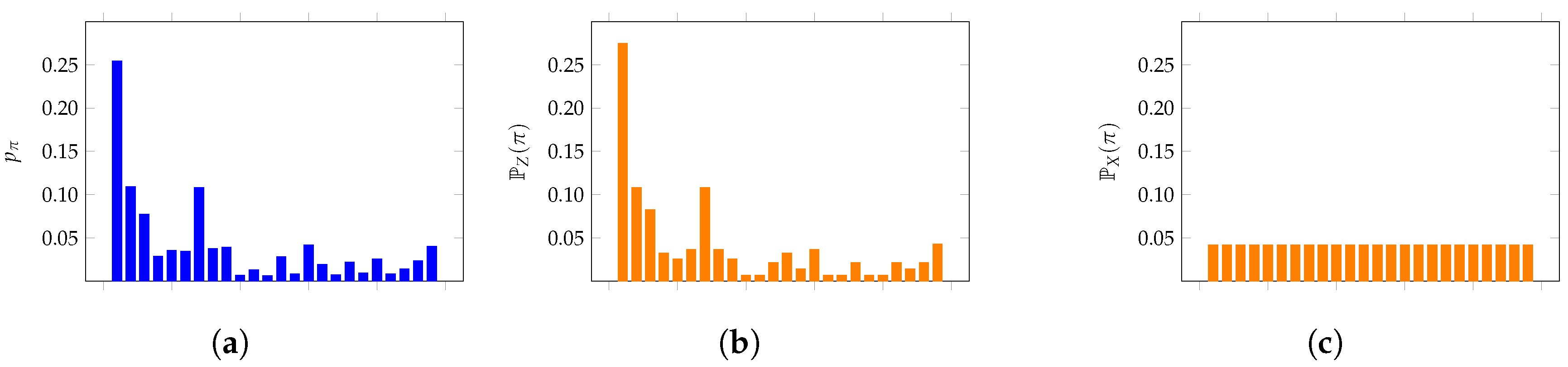
We begin by constructing a time series of length 2000 from a uniform random walk by fixing and compare the distribution of patterns of length four to the values derived from Section 2, as well as the uniform values of . Figure 3 displays these results: the observed distribution is plotted in blue (a), while the two possible null models, i.e., the random walk null model (b) and the uniform distribution of patterns (c), are plotted in orange.
As expected, the observed values match the null model distributions much more closely than the uniform distribution. Note that the expected and observed values on the left do not match exactly because the empirical time series has a finite length. This is a common feature of time series data that is observed throughout this paper.
We next consider a similar analysis for economic market data, using the daily closing prices of the S&P 500 over a seven-year period (). For this example, we need to estimate an underlying distribution. To do this, we calculate the sequence of steps (called the stock returns) and find the best fit normal curve; in this case, obtaining parameters = (0.702, 14.945). The null model for S&P 500 is the distribution of patterns for the normal random walk with these parameters. Using a simulated normal random walk, we approximate the distribution of patterns for a fixed n. This null model is shown in Figure 4 for n = 4, 5, and again, these data display a non-uniform distribution similar to those in Figure 2 and Figure 3. This reinforces our conclusion that modeling some time series with random walk null models more effectively describes the behavior than does the uniform distribution.
This example was computed with respect to a particular random walk null model; however, there are many options for the distribution of steps Y. A discussion of the possible inferential processes for selecting Y given a particular dataset is beyond the scope of this paper. However, for the purposes of comparing to permutation entropy, we consider several difference choices of Y and compare their performance to the uniform distribution. These results are summarized in Figure 5 below.
We compare the distributions derived from the actual S&P 500 data to three random walk null models: (a) the normally-distributed model described above with , (b) a uniform model with and (c) a uniform model fitting the stock returns with . The error between the expected values and the empirical values is shown for each permutation in Figure 5. Notice that each of the random walk models significantly outperforms the uniform distribution. The sum of squared errors for the uniform distribution of patterns is 0.0213 and for each of the models is (a) 0.0018, (b) 0.0027 and (c) 0.0031. Although there is some variance among the random walk models across the permutations, they each convincingly outperform the uniform one.
5. Data Descriptions
Throughout the remainder of this paper, we use several example datasets to evaluate our methods and compare to traditional approaches. Unless otherwise specified, these time series have data points. These data include synthetic random values, as well as empirical data from economics, ecology and medicine. Below, we describe the key features of the data and the abbreviations that we use throughout the paper. Plots of the time series are displayed in Figure A1 Appendix C.
- RAND: A sequence of 2000 uniform random numbers drawn between zero and one;
- NORM RW: A simulated random walk whose steps are drawn at random from the standard normal distribution, ;
- N-DRIFT RW: A simulated random walk whose steps are drawn at random from the normal distribution with ; this is the normal curve fitted to the returns in the S&P 500 data below.
- UNIF RW: A simulated random walk whose steps are drawn uniformly at random from the uniform distribution on the interval ;
- SP500: The daily closing values of the S&P 500 from 24 January 2009–31 December 2016. Data provided by Morningstar and accessed through [31];
- MEX: Average daily temperatures in Mexico City from 20 June 2011–31 December 2016. Data provided by the World Meteorological Organization through [31];
- NYC: Average daily temperatures in New York City from 20 June 2011–31 December 2016; data provided by the National Oceanic and Atmospheric Administration through [31];
- HEART: Instantaneous heart rate measurements taken at s intervals collected at the Massachusetts Institute of Technology [32].
In all cases, random values are generated using Mathematica’s [31] pseudo-random number generator, and all historical market closing values are provided by Morningstar through Mathematica. In the final section, we use the daily closing prices of the S&P 500, Apple (AAPL), Amazon (AMZN), Bank of America (BAC), General Electric (GE), Coca Cola (KO) and United Parcel Service of America (UPS), for trading days from 1 January 2002–1 January 2017 (). Finally, for a longitudinal test, we use daily closing prices of the S&P 500 from 1 January 1958–1 January 2017 ().
Table 1 gives the permutation entropy and missing patterns of several different types of datasets for small values of n. Of particular interest is the fact that missing patterns appear in all datasets for , even those that are guaranteed asymptotically to contain all patterns. Additionally, notice that the permutation entropy values are quite large for many of the noisy and random datasets.
6. Applications of KL Divergence Method
In order to directly compare our results to permutation entropy, we computed and for each of the datasets RAND, HEART, MEX, NYC, SP500, GE and NORM RW. The results are displayed in Figure 6. The permutation entropy is plotted in Figure 6a and the random walk KL divergence in Figure 6b.
This supports our view that the KL divergence method is frequently a better measure of deviation from a random walk than permutation entropy. The weather datasets are an interesting example in which the structure is periodic and hence neither uniformly random, nor a fixed random walk. Thus, we see moderate performance under both measures. However, notice that only slightly distinguishes temperature data and a simulated random walk, but the measure clearly separates them.
To add context to the value of the KL divergence, we simulated 400 random walks, , associated with X of length N and calculated for each. Using these simulations, we calculate the mean and standard deviation of the KL divergence of the simulated random walks against the model. These are plotted in Figure 6b. Notice that the stock data are much better approximated by the random walk of its steps than any of the other time series.
Finally, in order to determine how the length of the time series affects , we simulate a symmetric uniform random walk, , of length N and compare it to the distribution of patterns in the random walk, as derived in Section 2. The results mirror those of Figure 6. For of length , and . For of length , , where it remains for larger N, , and falling to when . This is expected behavior as the value goes to zero in the limit.
Expanding on our remarks from the previous section, permutation entropy has frequently been used to study financial time series. For instance, permutation entropy and the number of forbidden patterns for both closing values and returns were suggested as methods for distinguishing developed and emerging markets with the aim of using these measures to quantify stock market inefficiency [8]. In this analysis, permutation entropy of returns was correlated with either being a developed or an emerging market, with emerging markets having smaller permutation entropy (i.e., more correlation). We plot these values for our datasets below in Figure 7. Notice that the changes in heart rate are more correlated than steps in the other time series investigated here. We perform a more direct comparison of these two approaches in the following section.
A careful analysis of this method demonstrates some key features that lead us to prefer the explicit random walk model. First, we note that this measure assigns very low values to all of the stock data. As we will see in the next section, this property limits the amount of information that can be extracted. Secondly, we note that the measure does not clearly distinguish the periodic weather data from the random walks. Finally, the permutation entropy of the steps discovers a relatively high value for i.i.d. randomly drawn data points because the differences between the random variables is not independent.
7. Inefficiency in Financial Markets
In this final section, we analyze the stock market data more closely using the KL method and measure of momentum introduced above. The economic heuristic suggests that the most appropriate model of the stock market is that of the random walk; see for example [19]. Moreover, since a market whose prices are modeled by a random walk is considered efficient, the divergence of a market from that of a random walk serves as a measure of inefficiency [19]. Quantifying market inefficiency is an important and well-studied question in finance. Applying our method from Section 3 to a variety of stocks, we posit that a measure of inefficiency using the KL divergence from a random walk null model is preferable to the permutation entropy of returns. First, using the measures:
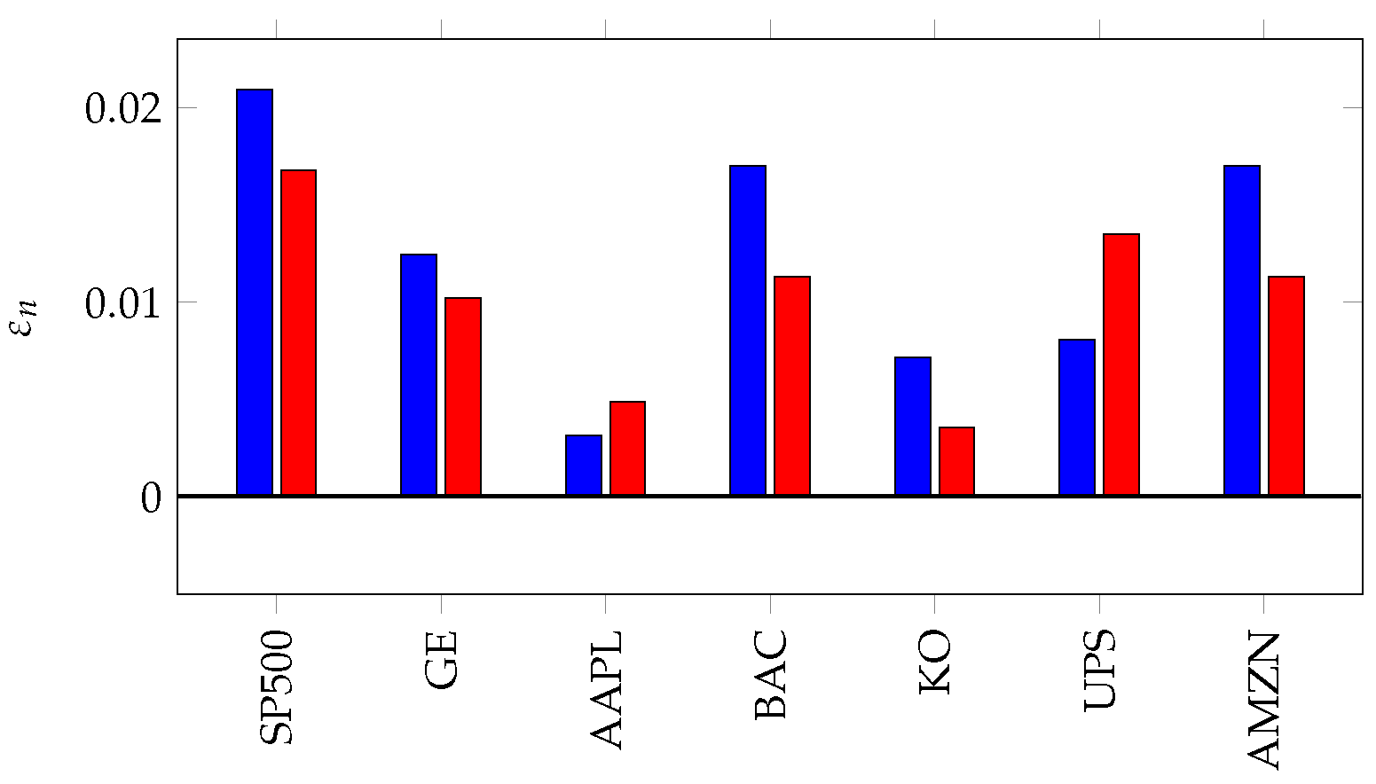
that we developed in Section 3.1, we capture the momentum phenomena observed in financial markets. Indeed, suggests a presence of upward momentum and suggests a presence of downward momentum. As depicted in Figure 8, for each of the stocks considered, the values of and are positive, suggesting the presence of both upward and downward momentum in these markets. Both of these results accord with economic data reported by the National Bureau of Economic Research [33,34].
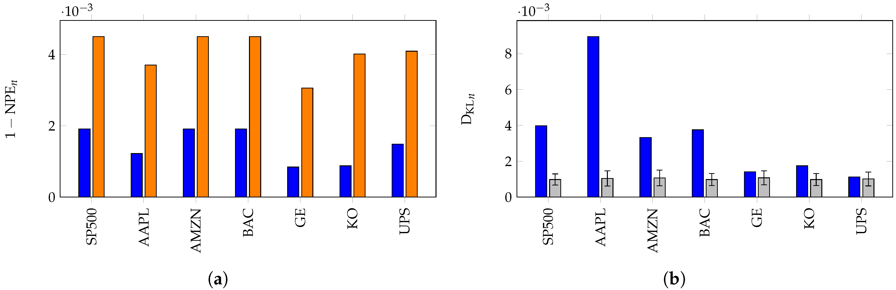
Although the previous result suggests that a random walk may not capture all of the information about the stock behavior since the momentum is a measure of the correlation of the steps, which we have assumed to be i.i.d., we conclude with two examples demonstrating the advantages of the random walk divergence over the permutation entropy of returns. For each of the stocks under consideration, we form 400 random walks, , associated with X of length (the length of X). Then, to determine the significance of , we compute for each.
The results of this experiment are presented in Figure 9. It is clear from the figure that Apple stock (AAPL) is furthest from a random walk, perhaps a result of calendar year phenomena associated the release of new products. On the other hand, large industrial stocks such as General Electric, Coke and United Parcel Service (respectively GE, KO and UPS) adhere more closely to the random walk model and are considered more efficient markets in this analysis.
As a final application of these methods, we use historical S&P500 closing prices from January 1958–January 2017 and plot our measure of inefficiency, , over time, comparing to the permutation entropy of the steps. For each year from 1960–2014, for the five-year range surrounding the year (i.e., from 1 January of two years prior to 31 December of two years after, ), we compute for the S&P500 in Figure 10 below.
The general trends depicted in the plot of resonate with the evolution of technology and economic events of that time, while the permutation entropy of the steps is less informative. In particular, we can see the decline in inefficiency as a result of computerized trading, as well as the stock market crash of 1989, the 2000 technology bubble and the 2008 financial crisis causing an increase in variability and distance from the model. The results presented here are similar to those in [4] for the Shanghai and Shenzhen Stock Exchanges.
8. Summary and Conclusions
In order to account for the observed behavior of the distribution of ordinal patterns in time series from economics and other fields, we have introduced a measure of complexity based on random walk null models. Since much of the structure of the ordinal patterns appearing in these financial time series is explained by the underlying process of a random walk, this measure is better suited for such time series than previous methods based on permutation entropy. We provided theoretical and numerical results on the distribution of patterns in the context of random walk models and provided a set of tools for analyzing the complexity of data modeled by time series. Additionally, we have applied our methods to examples from several different domains in order to validate their usefulness.
Based on our experiments, we conclude that the methods introduced in this paper offer significant advantages for analyzing and understanding the structure in random walk time series. Not all time series data plausibly arise from random walk processes, but for those that do, the methods presented in this paper provide a principled method for studying their complexity and inefficiency.
Acknowledgments
The authors would like to express their gratitude to Peter Doyle, Sergi Elizalde, Nishant Malik, Megan Martinez, Scott Pauls and Dan Rockmore for their helpful comments and guidance. Additionally, the authors thank the anonymous peer reviewers for their insightful comments and helpful advice.
Author Contributions
Daryl DeFordand Katherine Moore conceived of and designed the experiments, performed the experiments, analyzed the data and wrote the paper collaboratively. Both authors have read and approved the final manuscript.
Conflicts of Interest
The authors declare no conflict of interest.
Abbreviations
The following abbreviations are used in this manuscript:
| KL | Kullback–Liebler |
| PE | Permutation Entropy |
| NPE | Normalized Permutation Entropy |
Appendix A. Null Model Distributions
Here, we give the expected distributions of ordinal patterns for the uniform and normal random walk models as described in Section 2. Recall that for the normal distribution, the values do not depend on the variance when the mean is zero. For the uniform distribution, the case is equivalent to setting . The classes of patterns that are grouped together in the leftmost column must always occur with the same probability in any random walk model [30].

Table A1.
The values of for the normal distribution with and in the uniform case for , where .
| Pattern | Normal: | Uniform: | Uniform: |
|---|---|---|---|
| {123} | |||
| {132, 213} | |||
| {231, 312} | |||
| {321} | |||
| {1234} | 0.1250 | ||
| {1243, 2134} | 0.0625 | 1/16 | |
| {1324} | 0.0417 | 1/24 | |
| {1342, 3124} | 0.0208 | 1/24 | |
| {1423, 2314} | 0.0355 | 1/48 | |
| {1432, 2143, 3214} | 0.0270 | 1/48 | |
| {2341, 3412, 4123} | 0.0270 | 1/48 | |
| {2413} | 0.0146 | 1/48 | |
| {2431, 4213} | 0.0208 | 1/24 | |
| {3142} | 0.0146 | 1/48 | |
| {3241, 4132} | 0.0355 | 1/48 | |
| {3421, 4312} | 0.0625 | 1/16 | |
| {4231} | 0.0417 | 1/24 | |
| {4321} | 0.1250 | 1/8 |
Appendix B. Permutation Equivalence Classes
In [27,30], the authors defined equivalence relation on permutations by if for any random walk, Z. They show that if the permutations can be related by a sequence of combinatorial moves. For completeness, we list the equivalence classes described by their result. Although the existence of these classes was categorized theoretically, we believe this is the first time they have been explicitly computed [27]. These classes are used to define the function in Section 3.1.
For , the classes are:
For , the classes are:
For , the classes are:
Appendix C. Data Plots
In this Appendix, we display plots of the datasets described in Section 5 and used throughout the paper. Plots were generated with Mathematica [31].
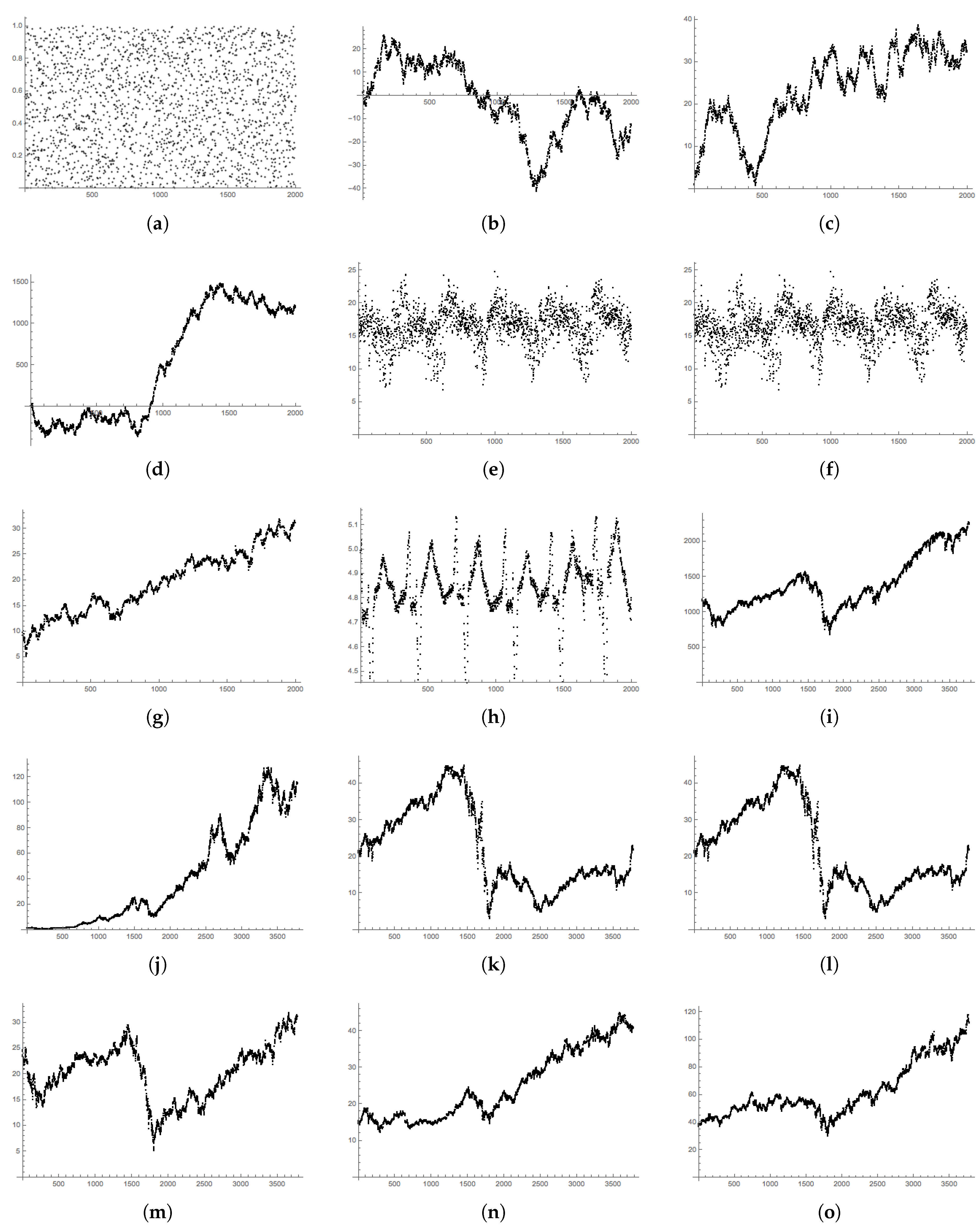
Figure A1.
Graphs of the time series used throughout this paper; see Section 5. Time series (a–h) are of length . Stock data (i–o), used in Section 7, are closing prices for trading days from 1 January 2002–1 January 2017 and of length . (a) RAND; (b) NORM RW; (c) UNIF RW; (d) N-DRIFT RW; (e) MEX; (f) NYC; (g) GE; (h) HEART; (i) StockSP500; (j) Stock AAPL; (k) Stock AMZN; (l) Stock BAC; (m) Stock GE; (n) Stock KO; (o) Stock UPS.

References
- Amigó, J.M.; Zambrano, S.; Sanjuán, M.A.F. Combinatorial detection of determinism in noisy time series. Europhys. Lett. 2008, 83, 60005. [Google Scholar] [CrossRef]
- Bandt, C. Autocorrelation type functions for big and dirty data series. arXiv, 2014; arXiv:1411.3904. [Google Scholar]
- Bariviera, A.F.; Zunino, L.; Guercio, M.B.; Martinez, L.B.; Rosso, O.A. Revisiting the European sovereign bonds with a permutation-information-theory approach. Eur. Phys. J. B 2013, 86, 509. [Google Scholar] [CrossRef]
- Hou, Y.; Liu, F.; Gao, J.; Cheng, C.; Song, C. Characterizing Complexity Changes in Chinese Stock Markets by Permutation Entropy. Entropy 2017, 19, 514. [Google Scholar] [CrossRef]
- Lim, J.R. Rapid Evaluation of Permutation Entropy for Financial Volatility Analysis—A NovelHash Function using Feature-Bias Divergence. Available online: https://www.doc.ic.ac.uk/teaching/distinguished-projects/2014/j.lim.pdf (accessed on 15 Novermber 2017).
- Ortiz-Cruz, A.; Rodriguez, E.; Ibarra-Valdez, C.; Alvarez-Ramirez, J. Efficiency of crude oil markets: Evidences from informational entropy analysis. Energy Policy 2012, 41, 365–373. [Google Scholar] [CrossRef]
- Zunino, L.; Bariviera, A.F.; Guercio, M.B.; Martinez, L.B.; Rosso, O.A. On the efficiency of sovereign bond markets. Phys. A Stat. Mech. Appl. 2012, 391, 4342–4349. [Google Scholar] [CrossRef]
- Zunino, L.; Zanin, M.; Tabak, B.M.; Pérez, D.G.; Rosso, O.A. Forbidden patterns, permutation entropy and stock market inefficiency. Phys. A Stat. Mech. Appl. 2009, 388, 2854–2864. [Google Scholar] [CrossRef]
- Li, D.; Li, X.; Liang, Z.; Voss, L.J.; Sleigh, J.W. Multiscale permutation entropy analysis of EEG recordings during sevoflurane anesthesia. J. Neural Eng. 2010, 7, 1–4. [Google Scholar] [CrossRef] [PubMed]
- Li, X.; Ouyang, G.; Richards, D.A. Predictability analysis of absence seizures with permutation entropy. Epilepsy Res. 2007, 77, 70–74. [Google Scholar] [CrossRef] [PubMed]
- Liu, T.; Yao, W.; Wu, M.; Shi, Z.; Wang, J.; Ning, X. Multiscale permutation entropy analysis of electrocardiogram. Phys. A Stat. Mech. Appl. 2017, 471, 492–498. [Google Scholar] [CrossRef]
- Nicolaou, N.; Georgiou, J. Detection of epileptic electroencephalogram based on permutation entropy and support vector machines. Expert Syst. Appl. 2012, 39, 202–209. [Google Scholar] [CrossRef]
- Olofsen, E.; Sleigh, J.W.; Dahan, A. Permutation entropy of the electroencephalogram: A measure of anaesthetic drug effect. Br. J. Anaesth. 2008, 101, 810–821. [Google Scholar] [CrossRef] [PubMed]
- Weck, P.J.; Schaffner, D.A.; Brown, M.R.; Wicks, R.T. Permutation entropy and statistical complexity analysis of turbulence in laboratory plasmas and the solar wind. Phys. Rev. E Stat. Nonlinear Soft Matter Phys. 2015, 91, 023101. [Google Scholar] [CrossRef] [PubMed]
- Zunino, L.; Pérez, D.G.; Martín, M.T.; Garavaglia, M.; Plastino, A.; Rosso, O.A. Permutation entropy of fractional Brownian motion and fractional Gaussian noise. Phys. Lett. A 2008, 372, 4768–4774. [Google Scholar] [CrossRef]
- Keller, K.; Mangold, T.; Stolz, I.; Werner, J. Permutation Entropy: New Ideas and Challenges. Entropy 2017, 19, 134. [Google Scholar] [CrossRef]
- Riedl, M.; Müller, A.; Wessel, N. Practical considerations of permutation entropy. Eur. Phys. J. Spec. Top. 2013, 222, 249–262. [Google Scholar] [CrossRef]
- Zanin, M.; Zunino, L.; Rosso, O.A.; Papo, D. Permutation entropy and its main biomedical and econophysics applications: A review. Entropy 2012, 14, 1553–1577. [Google Scholar] [CrossRef]
- Fama, E.F. The Behavior of Stock-Market Prices. J. Bus. 1965, 38, 34–105. [Google Scholar] [CrossRef]
- Fama, E.F. Random Walks in Stock Market Prices. Financ. Anal. J. 1995, 51, 75–80. [Google Scholar] [CrossRef]
- Bandt, C.; Shiha, F. Order Patterns in Time Series. J. Time Ser. Anal. 2007, 28, 646–665. [Google Scholar] [CrossRef]
- Sinn, M.; Keller, K. Estimation of ordinal pattern probabilities in Gaussian processes with stationary increments. Comput. Stat. Data Anal. 2011, 55, 1781–1790. [Google Scholar] [CrossRef]
- Bandt, C.; Pompe, B. Permutation entropy: A natural complexity measure for time series. Phys. Rev. Lett. 2002, 88, 174102. [Google Scholar] [CrossRef] [PubMed]
- Ouyang, G.; Dang, C.; Richards, D.A.; Li, X. Ordinal pattern based similarity analysis for EEG recordings. Clin. Neurophysiol. 2010, 121, 694–703. [Google Scholar] [CrossRef] [PubMed]
- Bandt, C. Permutation Entropy and Order Patterns in Long Time Series. In Time Series Analysis and Forecasting; Springer: Berlin, Germany, 2016; pp. 61–73. [Google Scholar]
- Kullback, S.; Leibler, R.A. On Information and Sufficiency. Ann. Math. Statist. 1951, 22, 79–86. [Google Scholar] [CrossRef]
- Martinez, M.; Elizalde, S. The frequency of pattern occurrence in random walks. In Proceedings of the 27th International Conference on Formal Power Series and Algebraic Combinatorics (FPSAC 2015), Discrete Mathematics & Theoretical Computer Science, DMTCS Proceedings, Daejeon, Korea, 6–10 July 2105. [Google Scholar]
- Kenyon, R.; Kral, D.; Radin, C.; Winkler, P. Permutations with fixed pattern densities. arXiv, 2015; arXiv:1506.02340. [Google Scholar]
- Elizalde, S.; Moore, K. Patterns of Negative Shifts and Beta-Shifts. arXiv, 2015; arXiv:1512.04479. [Google Scholar]
- Martinez, M.A. Equivalences on Patterns in Random Walks. Ph.D. Thesis, Dartmouth College, Hanover, NH, USA, 2015. [Google Scholar]
- Wolfram Research, Inc. Mathematica, Version 11.2. Available online: http://support.wolfram.com/kb/472 (accessed on 15 Novermber 2017).
- Goldberger, A.L.; Rigney, D.R. Nonlinear Dynamics at the Bedside. In Institute for Nonlinear Science; Theory of Heart; Springer: New York, NY, USA, 1991; pp. 583–605. [Google Scholar]
- Jegadeesh, N.; Titman, S. Returns to Buying Winners and Selling Losers: Implications for Stock Market Efficiency. J. Financ. 1993, 48, 65–91. [Google Scholar] [CrossRef]
- Jegadeesh, N.; Titman, S. Profitability of Momentum Strategies: An Evaluation of Alternative Explanations. Natl. Bur. Econ. Res. 1999. [Google Scholar] [CrossRef]
Figure 1.
The regions of integration for patterns in uniform random walks for (a) and (b) , sketched here for .
Figure 1.
The regions of integration for patterns in uniform random walks for (a) and (b) , sketched here for .
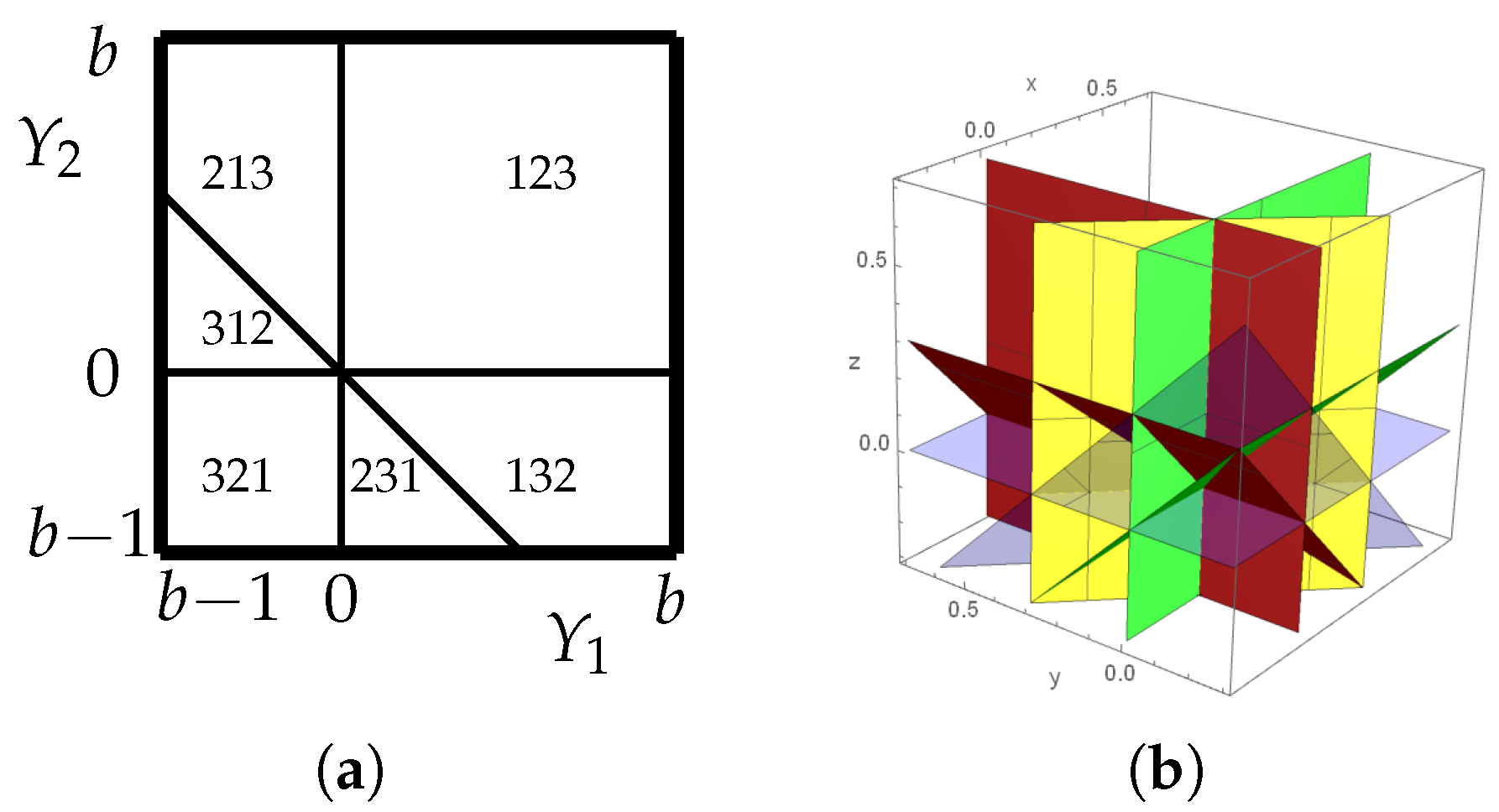
Figure 2.
The distribution of patterns of length , listed in lexicographical order , for (a) the normal random walk with , (b) the uniform random walk with and (c) the uniform random walk with .
Figure 2.
The distribution of patterns of length , listed in lexicographical order , for (a) the normal random walk with , (b) the uniform random walk with and (c) the uniform random walk with .
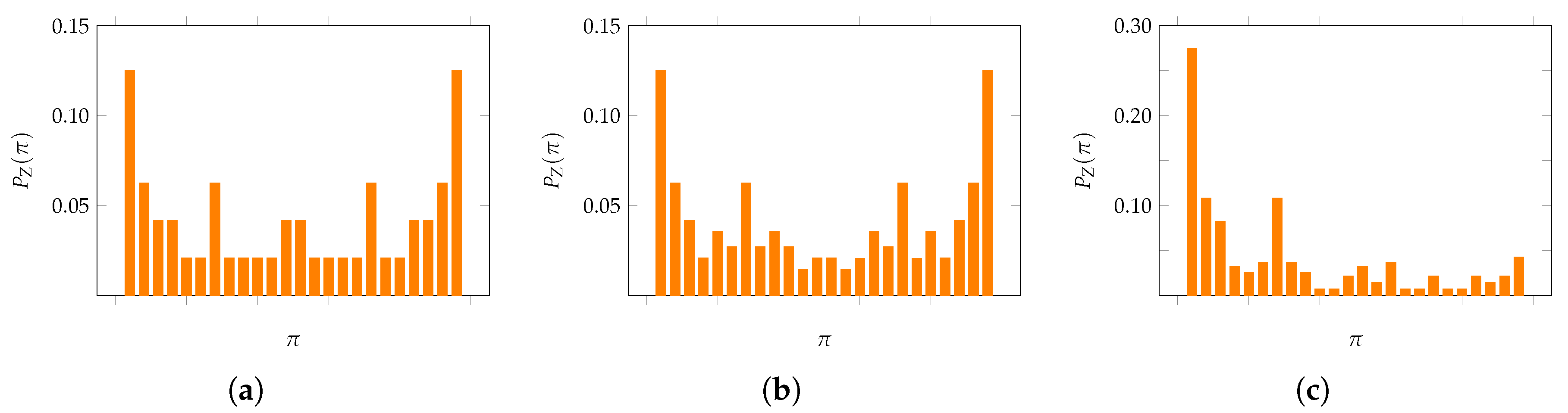
Figure 3.
The distribution of patterns of length in a length 2000 uniform random walk with (a). The true distribution of patterns in the uniform random walk with (b) is a much closer fit than the uniform distribution of patterns in white noise (c).
Figure 3.
The distribution of patterns of length in a length 2000 uniform random walk with (a). The true distribution of patterns in the uniform random walk with (b) is a much closer fit than the uniform distribution of patterns in white noise (c).

Figure 4.
The distribution of patterns, listed in lexicographical order, for the uniform random walk null model for closing prices in the S&P 500 of length (a) and (b) . Note that the distributions are far from uniform as is characteristic of random walk data.
Figure 4.
The distribution of patterns, listed in lexicographical order, for the uniform random walk null model for closing prices in the S&P 500 of length (a) and (b) . Note that the distributions are far from uniform as is characteristic of random walk data.
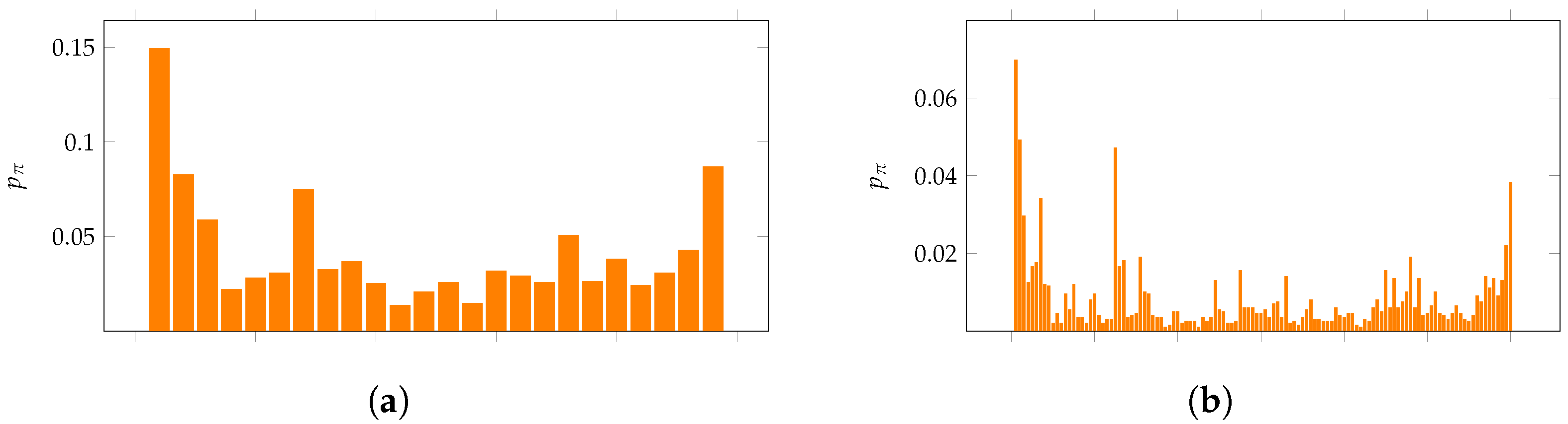
Figure 5.
Comparison of null model distributions for the S&P 500 data to the uniform distribution. The difference is plotted for each of the four null models: (orange), (blue), (red) and the uniform distribution (gray).
Figure 5.
Comparison of null model distributions for the S&P 500 data to the uniform distribution. The difference is plotted for each of the four null models: (orange), (blue), (red) and the uniform distribution (gray).
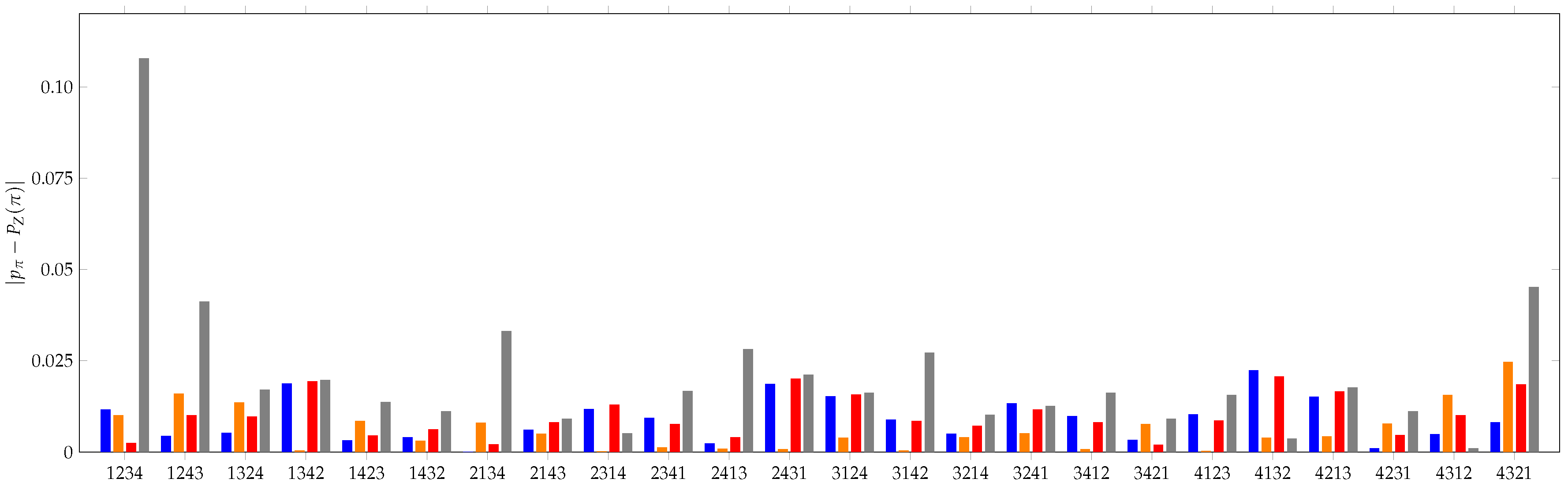
Figure 6.
In (a), we compute for the time series for (in blue) and (in orange). In (b), we compute for and the data of length (blue). We generate 400 random walks of length and compute for each. The mean and errors are plotted in gray.
Figure 6.
In (a), we compute for the time series for (in blue) and (in orange). In (b), we compute for and the data of length (blue). We generate 400 random walks of length and compute for each. The mean and errors are plotted in gray.
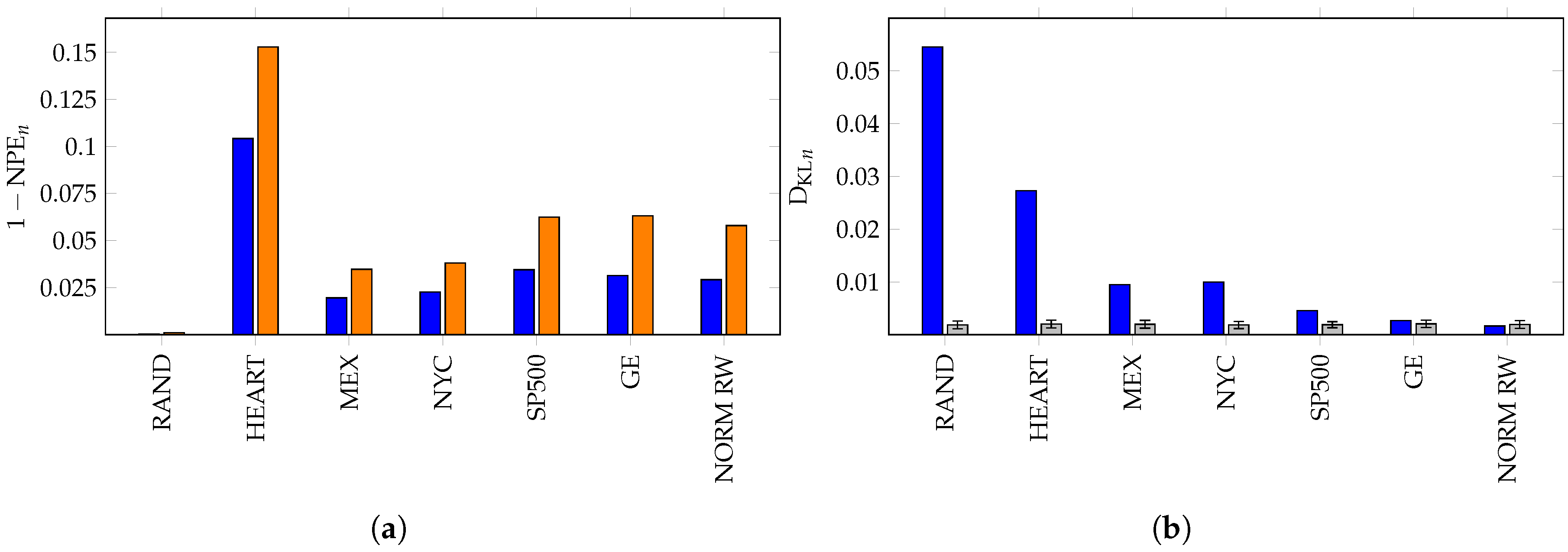
Figure 7.
We compute for the time series of steps for (in blue) and (in orange). This can be used as a measure of step independence and was presented in [5] as a measure of volatility in developing economic markets.
Figure 7.
We compute for the time series of steps for (in blue) and (in orange). This can be used as a measure of step independence and was presented in [5] as a measure of volatility in developing economic markets.
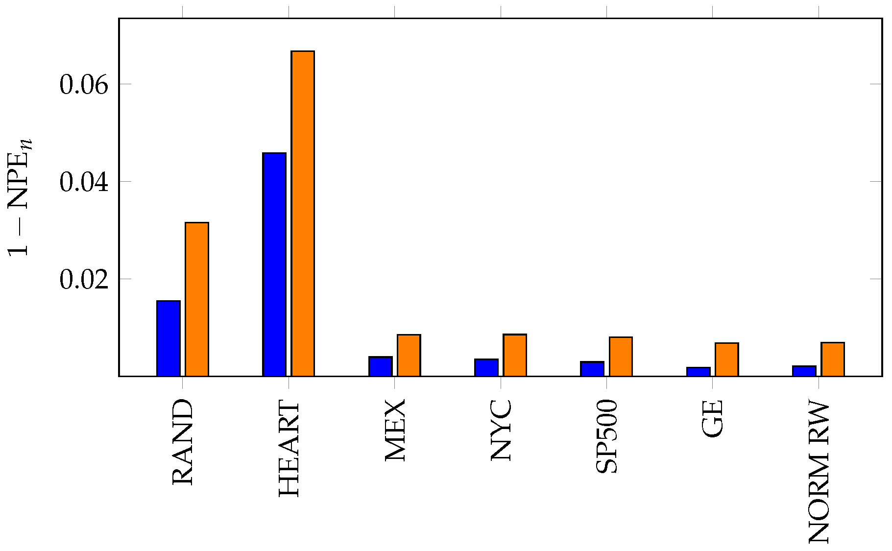
Figure 8.
Values of in blue and in red. Larger values of (respectively ) correspond to markets containing more increasing (respectively decreasing) runs than predicted by the independent steps of the random walk model.
Figure 8.
Values of in blue and in red. Larger values of (respectively ) correspond to markets containing more increasing (respectively decreasing) runs than predicted by the independent steps of the random walk model.

Figure 9.
In (a), we compute for the time series of steps for (in blue) and (in orange). In (b), we compute for and the data of length (blue). We generate 400 random walks (associated with X) of length and compute for each. The mean and errors are plotted in gray.
Figure 9.
In (a), we compute for the time series of steps for (in blue) and (in orange). In (b), we compute for and the data of length (blue). We generate 400 random walks (associated with X) of length and compute for each. The mean and errors are plotted in gray.

Figure 10.
Computation of (orange) and the permutation entropy of the steps (blue) on historical S&P500 daily closing prices during each five-year window surrounding the year on the x-axis. Both of these metrics can be treated as a proxy for inefficiency, but the provides significantly more information.

Table 1.
Computations of permutation entropy and the number of forbidden patterns for a range of time series of length described in Section 5. RAND, a sequence of 2000 uniform random numbers drawn between zero and one; N-DRIFT RW, a simulated random walk whose steps are drawn at random from the normal distribution with ; NORM RW, a simulated random walk whose steps are drawn at random from the standard normal distribution, ; UNIF RW, a simulated random walk whose steps are drawn uniformly at random from the uniform distribution on the interval ; MEX, average daily temperatures in Mexico City from 20 June 2011–31 December 2016.
| Data | Forbidden Patterns | Permutation Entropy | ||||
|---|---|---|---|---|---|---|
| RAND | 0 | 0 | 48 | 0.999 | 0.992 | 0.970 |
| NORM RW | 0 | 0 | 190 | 0.942 | 0.916 | 0.875 |
| N-DRIFT RW | 0 | 0 | 207 | 0.932 | 0.900 | 0.857 |
| UNIF RW | 0 | 0 | 216 | 0.930 | 0.899 | 0.855 |
| MEX | 0 | 0 | 129 | 0.965 | 0.952 | 0.926 |
| NYC | 0 | 0 | 115 | 0.962 | 0.950 | 0.924 |
| SP500 | 0 | 0 | 199 | 0.938 | 0.907 | 0.863 |
| GE | 0 | 2 | 210 | 0.937 | 0.906 | 0.863 |
| HEART | 0 | 8 | 344 | 0.847 | 0.813 | 0.777 |
© 2017 by the authors. Licensee MDPI, Basel, Switzerland. This article is an open access article distributed under the terms and conditions of the Creative Commons Attribution (CC BY) license (http://creativecommons.org/licenses/by/4.0/).
Share and Cite
MDPI and ACS Style
DeFord, D.; Moore, K. Random Walk Null Models for Time Series Data. Entropy 2017, 19, 615. https://doi.org/10.3390/e19110615
AMA Style
DeFord D, Moore K. Random Walk Null Models for Time Series Data. Entropy. 2017; 19(11):615. https://doi.org/10.3390/e19110615
Chicago/Turabian StyleDeFord, Daryl, and Katherine Moore. 2017. "Random Walk Null Models for Time Series Data" Entropy 19, no. 11: 615. https://doi.org/10.3390/e19110615
Note that from the first issue of 2016, this journal uses article numbers instead of page numbers. See further details here.