Variational Characterization of Free Energy: Theory and Algorithms

Abstract

The article surveys and extends variational formulations of the thermodynamic free energy and discusses their information-theoretic content from the perspective of mathematical statistics. We revisit the well-known Jarzynski equality for nonequilibrium free energy sampling within the framework of importance sampling and Girsanov change-of-measure transformations. The implications of the different variational formulations for designing efficient stochastic optimization and nonequilibrium simulation algorithms for computing free energies are discussed and illustrated.

1. Introduction

It is one of the standard problems in statistical physics and its computational applications, e.g., in molecular dynamics, that one desires to compute expected values of an observable f with respect to a given (equilibrium) probability density $\pi$,

$${\mathbf{E}}_{\pi }\left[f\right]=\int f\left(x\right)\pi \left(x\right)dx$$

Even if samples from the density $\pi$ are available, the simplest Monte Carlo estimator, the mean value, may suffer from a large variance (compared to the quantity that one tries to estimate), such that the accurate estimation of ${\mathbf{E}}_{\pi }\left[f\right]$ requires an unreasonably large sample size. Various approaches to circumvent this problem and to reduce the variance of an estimator are available, one of the most prominent representatives being importance sampling where samples are drawn from another probability density $\rho$ and reweighted with the likelihood ratio $\pi /\rho$ [1,2]. It is well-known that theoretically (and under certain assumptions) there exists an optimal importance sampling density ${\rho }^{\ast }$ such that the resulting estimator has variance zero. By a clever choice of the importance sampling proposal density, it is thus possible to completely remove the stochasticity from the problem and to obtain what is sometimes called certainty equivalence. Yet, drawing samples from the optimal density (or an approximation of it) is a difficult problem in itself, so that the striking variance-reduction due to importance sampling often does not pay off in practice.

The zero variance property of importance sampling and the challenge to utilize it algorithmically is the starting point of this article where the focus is on its generalization to path sampling problems and its algorithmic realization. Regarding the former, we will show that the Donsker–Varadhan variational principle, a well-known measure-theoretic characterization of the cumulant generating functions [3] that gives rise to a variational characterization of the thermodynamic free energy [4,5] permits several stunning utilizations of the importance sampling framework for path sampling problems; examples involve trajectory-dependent expectations like expected hitting times or free energy differences [6,7]. We will see that finding the optimal change of measure in path space is equivalent to solving an optimal control problem for the underlying dynamical system in which the dynamics is controlled by external driving forces and thus driven out of equilibrium [8,9].

One of the central contributions of this paper is that we prove that the resulting path space importance sampling scheme features zero variance estimators under quite general assumptions. We furthermore elaborate on the connection between optimized importance sampling and the famous Jarzynski fluctuation relation for the thermodynamic free energy [10]. In particular we will explore this connection and describe how to devise better non-equilibrium free energy algorithms, and hopefully obtain a better understanding of Jarzynski-based estimators; cf. [11,12,13,14].

Regarding the algorithmic realization, the theoretical insight into the relation between (adaptive) importance sampling and optimal control leads to novel algorithms that aim at utilizing the zero variance property without having to sample from the optimal importance sampling density. We will demonstrate how this can be achieved by discretizing the optimal control problem, using ideas from stochastic approximation and stochastic optimization [9,15]; see [16,17,18] for an alternative approach using ideas from the theory of large deviations. The examples we present are mainly pedagogical and admittedly very simple, but they highlight important features of the importance sampling scheme, such as the exponential tilting of the (path space) probability measure or the uniqueness of the solution to the stochastic approximation problem within a certain parametric family of trial probability measures, and this is why we confine our attention to such low-dimensional examples. Regarding the application of our approach to molecular dynamics simulation, we allude to the relevant literature.

Outline

The article is organized as follows: Firstly, in Section 2 we review certainty equivalence and the zero variance property of optimized importance sampling in state space, starting from the Donsker–Varadhan principle and its relation to importance sampling, and comment on some algorithmic issues. Then, in Section 3, we consider the generalization to path space, discuss the relation to stochastic optimal control and revisit Jarzynski-based estimators for thermodynamic free energies. Section 4 surveys and discusses novel algorithms that are exploiting the theoretical properties of the control-based importance sampling scheme. We briefly discuss some of these algorithms with simple toy examples in Section 5, before the article concludes in Section 6 with a brief summary and a discussion of open issues. The article contains four appendices that record various technical identities, including a brief derivation of Girsanov’s change of measure formula, and the proof of the main theorem: the zero-variance property of optimized importance sampling on path space.

2. Certainty Equivalence

In mathematical finance, the guaranteed payment that an investor would accept instead of a potentially higher, but uncertain return on an asset is called a certainty equivalent. In physics, certainty equivalence amounts to finding a deterministic surrogate system that reproduces averages of certain fluctuating thermodynamic quantities with probability one. One such example is the thermodynamic free energy difference between two equilibrium states that can be either computed by an exponential average over the fluctuating nonequilibrium work done on the system or by measuring the work of an adiabatic transformation between these states.

2.1. Donsker–Varadhan Variational Principle

Before getting into the technical details, we briefly review the classical Donsker–Varadhan variational principle for the cumulant generating function of a random variable. To this end, let X be a real-valued, n-dimensional random variable with smooth probability density $\pi$ and call

$${\mathbf{E}}_{\pi }\left[f\left(X\right)\right]={\int }_{{\mathbb{R}}^n}f\left(x\right)\pi \left(x\right)dx$$

(1)

the expectation with respect to $\pi$ for any integrable function $f:{\mathbb{R}}^n\to \mathbb{R}$.

Definition 1.

Let $W:{\mathbb{R}}^n\to \mathbb{R}$ be a bounded random variable. The quantity

$$\gamma :\mathcal{B}\left({\mathbb{R}}^n\right)\to \mathbb{R},W\mapsto -log{\mathbf{E}}_{\pi }\left[exp(-W)\right]$$

(2)

is called the free energy of the random variable $W=W\left(X\right)$ with respect to π, where $\mathcal{B}\left({\mathbb{R}}^n\right)$ is the set of bounded and measurable, real-valued functions on ${\mathbb{R}}^n$ (“If you can write it down, it’s measurable!”, S. R. Srinivasa Varadhan).

Definition 2.

Let ρ be another probability density on ${\mathbb{R}}^n$. Then

$$D\left(\rho \right|\pi )={\int }_{{\mathbb{R}}^n}log\frac{\rho \left(x\right)}{\pi \left(x\right)}\rho \left(x\right)dx$$

(3)

is called the relative entropy of ρ with respect to π (or: Kullback–Leibler divergence), provided that $\pi \left(x\right)=0$ implies that $\rho \left(x\right)=0$ for every $x\in {\mathbb{R}}^n$. Otherwise, we set $D\left(\rho \right|\pi )=+\infty$.

The requirement that $\pi \left(x\right)$ must not be zero without $\rho \left(x\right)$ being zero is known as absolute continuity and guarantees that the likelihood ratio $L=\rho /\pi$ is well defined. In what follows, we may assume without loss of generality that $\pi >0$. (Otherwise we may exclude those states $x\in {\mathbb{R}}^n$ for which $\pi \left(x\right)=0$.)

A well-known thermodynamic principle states that the free energy is the Legendre transform of the entropy. The following variant of this principle is due to Donsker and Varadhan and says that (e.g., see [3] and the references therein)

$$-log{\mathbf{E}}_{\pi }\left[exp(-W)\right]=\underset{\rho \ge 0}{min}\left\{{\mathbf{E}}_{\rho }\left[W\right]+D\left(\rho \right|\pi )\right\},$$

(4)

where the minimum is over all probability density functions $\rho$ on ${\mathbb{R}}^n$. The last equality easily follows from Jensen’s inequality by noting that

$$\begin{array}{cc}\hfill -log{\int }_{{\mathbb{R}}^n}exp(-W)\pi dx& =-log{\int }_{{\mathbb{R}}^n}exp(-W)\frac{\pi }{\rho }\rho dx\hfill \\ & =-log{\int }_{{\mathbb{R}}^n}exp\left(-W-log\frac{\rho }{\pi }\right)\rho dx\hfill \\ & \le {\int }_{{\mathbb{R}}^n}\left(W+log\frac{\rho }{\pi }\right)\rho dx\hfill \\ & ={\int }_{{\mathbb{R}}^n}W\rho dx+{\int }_{{\mathbb{R}}^n}log\frac{\rho }{\pi }\rho dx.\hfill \end{array}$$

Additionally, it can be readily seen that equality is attained if and only if

$${\rho }^{\ast }=exp(\gamma -W)\pi ,$$

(5)

which defines a probability measure with $\gamma$ given in Equation (2).

Importance Sampling

The relevance of Equations (4) and (5) lies in the fact that, by sampling X from the probability distribution with density ${\rho }^{\ast }$, one removes the stochasticity from the problem, since the random variable

$$U^{\ast }=W\left(X\right)+log\frac{{\rho }^{\ast }\left(X\right)}{\pi \left(X\right)}$$

is almost surely (a.s.) constant. As a consequence, the Monte Carlo scheme for computing the free energy on the left hand side of Equation (4) based on the empirical mean of the independent draws of $U^{\ast }=U^{\ast }\left(X\right)$ with $X\sim {\rho }^{\ast }$, will have a zero variance. This zero-variance property is a consequence of Jensen’s inequality and the strict concavity of the logarithmic function which implies that equality is attained if and only if the random variable inside the expectation is almost surely constant. The next statement makes this precise.

Theorem 1 (Optimal importance sampling).

Let ${\rho }^{\ast }$ be the probability density given in Equation (5). Then the random variable $Z=exp(-W)\pi /{\rho }^{\ast }$ has zero variance under ${\rho }^{\ast }$, and we have:

$$Z={\mathbf{E}}_{\pi }[exp(-W)],{\rho }^{\ast }-\mathrm{a}.\mathrm{s}.$$

Proof. 

We need to show that ${\mathrm{Var}}_{{\rho }^{\ast }}\left(Z\right)={\mathbf{E}}_{{\rho }^{\ast }}\left[Z^2\right]-{\left({\mathbf{E}}_{{\rho }^{\ast }}\left[Z\right]\right)}^2=0$. Using Equation (5) and noting that ${\rho }^{\ast }>0$ since W is bounded and $\pi >0$, it follows that Z has finite second moment and

$$\begin{array}{cc}\hfill {\mathbf{E}}_{{\rho }^{\ast }}\left[Z^2\right]-{\left({\mathbf{E}}_{{\rho }^{\ast }}\left[Z\right]\right)}^2& ={\mathbf{E}}_{\pi }\left[exp(-2W)\pi /{\rho }^{\ast }\right]-{\left({\mathbf{E}}_{\pi }[exp(-W)]\right)}^2\hfill \\ & =exp(-\gamma ){\mathbf{E}}_{\pi }\left[exp(-W)\right]-exp(-2\gamma )\hfill \\ & =0,\hfill \end{array}$$

where we have used that $exp(-\gamma )={\mathbf{E}}_{\pi }[exp(-W)]$. ☐

The above theorem asserts that ${\rho }^{\ast }$-almost surely (${\rho }^{\ast }$-a.s.)

$$Z={\mathbf{E}}_{{\rho }^{\ast }}\left[Z\right],$$

(6)

which means that the importance sampling scheme based on estimating ${\mathbf{E}}_{{\rho }^{\ast }}\left[Z\right]$ using draws from the density ${\rho }^{\ast }$ is a zero-variance estimator of ${\mathbf{E}}_{\pi }[exp(-W)]$. We will discuss the problem of drawing from an approximation of the optimal distribution ${\rho }^{\ast }$ later on in Section 4.

Remark 1.

Equation (4) furnishes the famous relation $F=U-TS$ for the Helmholtz free energy F, with U being the internal energy, T the temperature and S denoting the Gibbs entropy. If we modify the previous assumptions by setting $\pi \equiv 1$ and $W=\beta E$ where $\beta ={\left(k_{B}T\right)}^{-1}$ with $k_B>0$ being Boltzmann’s constant and E denoting a smooth potential energy function that is bounded from below and growing at infinity, then

$$\underset{=F}{\underbrace{-{\beta }^{-1}log\int exp(-\beta E)dx}}=\underset{\rho >0}{min}\left\{\underset{=U}{\underbrace{\int E\rho dx}}+\underset{=-TS}{\underbrace{{\beta }^{-1}\int \rho log\rho dx}}\right\},$$

with the unique minimizer being the Gibbs-Boltzmann density ${\rho }^{\ast }=exp(-\beta E)/Z$ with normalization constant $Z=exp(-\beta F)$. In the language of statistics, ${\rho }^{\ast }$ is a probability distribution from the exponential family with sufficient statistic $E\left(X\right)$ and parameter $\beta >0$.

An alternative variational characterization of expectations is discussed in Appendix A.

2.2. Computational Issues

In practice, the above result is of limited use because the optimal importance sampling distribution is only known up to the normalizing constant C where the latter is just the sought quantity $C=exp(-\gamma )$. Clearly we can resort to Markov Chain Monte Carlo (MCMC) to generate samples ${\left({\widehat{Y}}_i\right)}_{i\ge 1}$ that are asymptotically distributed according to (see, e.g., [19])

$${\rho }^{\ast }\left(y\right)=\frac{exp(-\Phi (y\left)\right)}{C},\Phi \left(y\right)=V\left(y\right)+W\left(y\right).$$

However, in the situation at hand, we wish estimate ${\mathbf{E}}_{{\rho }^{\ast }}\left(Z\right)$ in Equation (6), where $Z=exp(-W)\pi /{\rho }^{\ast }$ is given in Theorem 1, and the problem is that the likelihood ratio $\pi /{\rho }^{\ast }$ is only known up to the normalizing factor. In this case, the self-normalized importance sampling estimator must be used (see, e.g., [20]):

$${\widehat{C}}_N=\frac{{\displaystyle \sum _{i=1}^{N}exp(-W\left({\widehat{Y}}_i\right))exp\left(W\left({\widehat{Y}}_i\right)\right)}}{{\displaystyle \sum _{i=1}^{N}exp\left(W\left({\widehat{Y}}_i\right)\right)}}=\frac{N}{{\displaystyle \sum _{i=1}^{N}exp\left(W\left({\widehat{Y}}_i\right)\right)}},$$

(7)

which is a consistent estimator for $C=exp(-\gamma )$. Note that unlike in the case of the importance sampling estimators with known likelihood ratio, the self-normalized estimator is only asymptotically unbiased, even if we can draw exactly from ${\rho }^{\ast }$ (see Appendix B for details.)

To avoid the bias due to the self-normalization, it is helpful to note that $exp\left(\gamma \right)={\mathbf{E}}_{{\rho }^{\ast }}[exp\left(W\right)]$ holds ${\rho }^{\ast }$-a.s. As a consequence,

$${\widehat{C}}_N^{-1}=\frac{{\displaystyle \sum _{i=1}^{N}exp\left(W\left({\widehat{Y}}_i\right)\right)}}{N}$$

(8)

is an unbiased estimator of $C^{-1}=exp\left(\gamma \right)$, provided that we can generate i.i.d. samples from ${\rho }^{\ast }$. Taking the logarithm, it follows that

$${\widehat{\gamma }}_N=-logN+log\left(\sum _{i=1}^{N}exp\left(W\left({\widehat{Y}}_i\right)\right)\right)$$

(9)

is a consistent estimator for $\gamma$, which by Jensen’s inequality and the strict concavity of the logarithm will again be only asymptotically unbiased.

Comparison with the Standard Monte Carlo Estimator

In most cases, the samples from ${\rho }^{\ast }$ will be generated by MCMC or the like. If we consider the advantages of ${\widehat{\gamma }}_N$ as compared to the plain vanilla Monte Carlo estimator

$${\tilde{\gamma }}_N=logN-log\left(\sum _{i=1}^{N}exp(-W\left({\widehat{X}}_i\right))\right),$$

(10)

with ${\left({\widehat{X}}_i\right)}_{i\ge 1}$ being a sample that is drawn from the reference distribution $\pi$, there are two aspects that will influence the efficiency of Equation (9) relative to Equation (10), namely:

(a)

the speed of convergence towards the stationary distribution and

(b)

the (asymptotic) variance of the estimator.

By construction, the asymptotic variance of the importance sampling estimator is zero or close to zero if we take numerical discretization errors into account, hence the efficiency of the estimator (9) is solely determined by the speed of convergence of the corresponding MCMC algorithm to the stationary distribution ${\rho }^{\ast }$, which, depending on the problem at hand, may be larger or smaller than the speed of convergence to $\pi$. It may even happen that $\pi$ is unimodal, whereas ${\rho }^{\ast }\propto e^{-W}\pi$ is multimodal and hence difficult to generate, for example when $\pi$ is the standard Gaussian density and $W={(x^2-d)}^2$ with $d\gg 0$ is a bistable (energy) function. We refrain from going into details here and instead refer to the review article [21] for an in-depth discussion of the asymptotic properties of reversible diffusions.

In Section 4 and Section 5, we discuss alternatives to Monte Carlo sampling based on stochastic optimization and approximation algorithms that are feasible even for large-scale systems.

Remark 2.

The comparison of Equations (9) and (10) suggests that the importance sampling estimator (9) is an instance of Bennett’s bidirectional estimator for a positive random variable, called “weighting function” in Bennett’s language [22]. As a consequence, Theorem 1 implies that Bennett’s bidirectional estimator has zero variance when the negative logarithm of the weighting function equals the bias potential.

3. Certainty Equivalence in Path Space

The previous considerations nicely generalize from the case of real-valued random variables to time-dependent problems and path functionals.

3.1. Donsker–Varadhan Variational Principle in Path Space

Let ${\left(X_s\right)}_{s\ge 0}$ with $X_0=x\in {\mathbb{R}}^n$ be the solution of the stochastic differential equation (SDE)

$$d{X}_s=b(X_s,s)ds+\sigma \left(X_s\right)d{B}_s,X_0=x,$$

(11)

where $b:{\mathbb{R}}^n\times [0,\infty )\to {\mathbb{R}}^n$ is a smooth, possibly time-dependent vector field, $\sigma :{\mathbb{R}}^n\to {\mathbb{R}}^{n\times m}$ is a smooth matrix field and B is an m-dimensional Brownian motion. Our standard example will be an SDE with $b(x,s)=-\nabla V\left(x\right)$ for a smooth potential energy function V and $\sigma \left(x\right)=\sqrt{2}{I}_{n\times n}$, so that $X_s$ satisfies a gradient dynamics. We assume throughout this paper that the functions $b,\sigma ,V$ are such that Equation (11) or the corresponding gradient dynamics have unique strong solutions for all $s\ge 0$.

Now, suppose that we want to compute the free energy (2) where W is now considered to be a functional of the paths $X=\{X_s:0\le s\le \tau \}$ for some bounded stopping time $\tau$:

$$W_{\tau }\left(X\right)={\int }_0^{\tau }f(X_s,s)ds+g\left(X_{\tau }\right),$$

(12)

for some bounded and sufficiently smooth, real valued functions $f,g$. We assume throughout the rest of the paper that $f,g$ are bounded from below and that W is integrable.

We define P to be the probability measure on the space $\Omega =C([0,\infty ),{\mathbb{R}}^n)$ of continuous trajectories that is induced by the Brownian motion ${\left(B_s\right)}_{s\ge 0}$ that drives the SDE (11). We call P a path space measure, and we denote the expectation with respect to P by ${\mathbf{E}}_P[·]$.

Definition 3 (Path space free energy).

Let ${\left(X_s\right)}_{s\ge 0}$ be the solution of Equation (11) and $W_{\tau }=W_{\tau }\left(X\right)\ge 0$ be integrable and defined by Equation (12). The quantity

$$\gamma =-log{\mathbf{E}}_P\left[exp(-W_{\tau })\right]=-log{\mathbf{E}}_P\left[exp\left(-{\int }_0^{\tau }f(X_s,s)ds-g\left(X_{\tau }\right)\right)\right]$$

(13)

is called the free energy of $W_{\tau }$ with respect to the path space measure P.

Note that Equation (13) simply is the path space version of Equation (2) which now implicitly depends on the initial condition $X_0=x$. The Donsker–Varadhan variational principle now reads

$$\gamma =\underset{Q\ll P}{inf}\left\{{\mathbf{E}}_Q\left[{\int }_0^{\tau }f(X_s,s)ds+g\left(X_{\tau }\right)\right]+D\left(Q\right|P)\right\},$$

(14)

where $Q\ll P$ stands for absolute continuity of Q with respect to P, which means that $P\left(E\right)=0$ implies that $Q\left(E\right)=0$ for any measurable set $E\subset \Omega$, as a consequence of which

$$D\left(Q\right|P)={\int }_{\Omega }log\frac{dQ}{dP}\left(\omega \right)dQ\left(\omega \right),$$

(15)

exists. Note that Equation (15) is just the generalization of the relative entropy (3) from probability densities on ${\mathbb{R}}^n$ to probability measures on the measurable space $(\Omega ,\mathcal{E})$, with $\mathcal{E}$ being a $\sigma$-algebra containing measurable subsets of $\Omega$, where we again declare that $D\left(Q\right|P)=\infty$ when Q is not absolutely continuous with respect to P. Therefore it is sufficient that the infimum in Equation (14) is taken over all path space measures $Q\ll P$.

If $W_{\tau }\ge 0$, it is again a simple convexity argument (see, e.g., [4]), which shows that the minimum in Equation (14) is attained at $Q^{\ast }$ given by:

$$\frac{d{Q}^{\ast }}{dP}{|}_{[0,\tau ]}=exp(\gamma -W_{\tau }),$$

(16)

where ${\phi |}_{[0,\tau ]}$ denotes the restriction of the path space density $\phi \left(X\right)=(d{Q}^{\ast }/dP)\left(X\right)$ to trajectories $X={\left(X_s\right)}_{s\ge 0}$ of length $\tau$. More precisely, ${\phi |}_{[0,\tau ]}$ is understood as the restriction of the measure $Q^{\ast }$ defined by $d{Q}^{\ast }=\phi dP$ to the $\sigma$-algebra ${\mathcal{F}}_{\tau }$ that contains all measurable sets $E\in \mathcal{E}$, with the property that for every $t\ge 0$ the set $E\cap \{\tau \le t\}$ is an element of the $\sigma$-algebra ${\mathcal{F}}_t=\sigma (X_s:0\le s\le t)$ that is generated by all trajectories ${\left(X_s\right)}_{0\le s\le t}$ of length t. In other words, ${\mathcal{F}}_{\tau }\subset \mathcal{E}$ is a $\sigma$-algebra that contains the history of the trajectories of (the random) length $\tau$.

Even though Equation (16) is the direct analogue of Equation (5), this result is not particularly useful if we do not know how to sample from $Q^{\ast }$. Therefore, let us first characterize the admissible path space measures $Q\ll P$ and discuss the practical implications later on.

3.1.1. Likelihood Ratio of Path Space Measures

It turns out that the only admissible change of measure from P to Q such that $D\left(Q\right|P)<\infty$ results in a change of the drift in Equation (11). Let ${\left(u_s\right)}_{s\ge 0}$ be an ${\mathbb{R}}^m$-valued stochastic process that is adapted, in that $u_t$ depends only on the Brownian motion $B_s$ up to time $s\le t$, and that satisfies the Novikov condition (see, e.g., [23]):

$${\mathbf{E}}_P\left[exp\left(\frac{1}{2}{\int }_0^{\tau }{\left|u_s\right|}^{2}ds\right)\right]<\infty .$$

(17)

Now, define the auxiliary process

$$B_t^u=B_t-{\int }_0^t{u}_{s}ds.$$

Using the definition of $B_t^u$, we may write Equation (11) as

$$d{X}_s=\left(b(X_s,s)+\sigma \left(X_s\right)u_s\right)ds+\sigma \left(X_s\right)d{B}_s^u,X_0=x.$$

(18)

Note that Equations (11) and (18) govern the same process ${\left(X_s\right)}_{s\ge 0}$, because the extra drift $\sigma (·)u$ is absorbed by the shifted mean of the process ${\left(\sigma \left(X_s\right)B_s^u\right)}_{s\ge 0}$. By construction, ${\left(B_s^u\right)}_{s\ge 0}$ is not a Brownian motion under P, because its expectation with respect to P is not zero in general. On the other hand, ${\left(B_s\right)}_{s\ge 0}$ is a Brownian motion under the measure P, and our aim is to find a measure $Q\ll P$ under which ${\left(B_s^u\right)}_{s\ge 0}$ is a Brownian motion. To this end, let ${\left(Z_s^u\right)}_{s\ge 0}$ be the process defined by

$$Z_t^u={\int }_0^t{u}_s·d{B}_s-\frac{1}{2}{\int }_0^t{\left|u_s\right|}^{2}ds,$$

(19)

or, equivalently,

$$Z_t^u={\int }_0^t{u}_s·d{B}_s^u+\frac{1}{2}{\int }_0^t{\left|u_s\right|}^{2}ds.$$

(20)

Girsanov’s theorem (see, e.g., [23], Theorem 8.6.4, or Appendix C) now states that ${\left(B_s^u\right)}_{0\le s\le \tau }$ is a standard Brownian motion under the probability measure Q with likelihood ratio

$$\frac{dQ}{dP}{|}_{[0,\tau ]}=exp\left(Z_{\tau }^u\right)$$

(21)

with respect to P where the Novikov condition (17) guarantees that ${\mathbf{E}}_P[exp\left(Z_{\tau }^u\right)]=1$, i.e., that Q is a probability measure. Inserting Equations (20) and (21) into the Donsker–Varadhan formula Equation (14), using that $B_s^u$ is Brownian motion with respect to Q, it follows that the term in $Z_{\tau }^u$ in the expression of the relative entropy, which is linear in u, drops out, and what remains is (cf. [4,6]):

$$\gamma =\underset{u}{inf}{\mathbf{E}}_Q\left[{\int }_0^{\tau }\left(f(X_s,s)+\frac{1}{2}{\left|u_s\right|}^2\right)ds+g\left(X_{\tau }\right)\right],$$

with $X_s$ being the solution of Equation (18). Since the distribution of $B^u$ under Q is the same as the distribution of B under P, an equivalent representation of the last equation is

$$\gamma =\underset{u}{inf}{\mathbf{E}}_P\left[{\int }_0^{\tau }\left(f(X_s^u,s)+\frac{1}{2}{\left|u_s\right|}^2\right)ds+g\left(X_{\tau }^u\right)\right].$$

(22)

where $X_s^u$ is the solution of the controlled SDE

$$d{X}_s^u=\left(b(X_s^u,s)+\sigma \left(X_s^u\right)u_s\right)ds+\sigma \left(X_s^u\right)d{B}_s,X_0^u=x,$$

(23)

with $B_s$ being our standard, m-dimensional Brownian motion (under P). See Appendix C for a sketch of derivation of Girsanov’s formula.

3.1.2. Importance Sampling in Path Space

Similarly to the finite dimensional case considered in the last section, we can derive optimal importance sampling strategies from the Donsker–Varadhan principle. To this end, we consider the case that $\tau$ is a random stopping time, which is a case that is often relevant in applications (e.g., when computing transition rates or committor functions [7]), but that is rarely considered in the importance sampling literature. Let $T>0$ and $O\subset {\mathbb{R}}^n$ be an open and bounded set with smooth boundary $\partial O$. We define

$${\tau }_O=inf\{s>0:X_s^u\notin O\},$$

as the first exit time of the set O and define the stopping time

$$\tau ={\tau }_O\wedge T$$

(24)

to be the minimum of ${\tau }_O$ and T, i.e., the exit from the set O or the end of the maximum time interval, whatever comes first. For the ease of notation, we will use the same symbol $\tau$ to denote the stopping time under the controlled or uncontrolled process (i.e., for $u=0$) throughout the article. Unless otherwise noted, it should be clear from the context whether $\tau$ is understood with respect to $X^u$ or $X=X^{u=0}$. Here, $X_s^u$ satisfies the controlled SDE (23).

We will argue that the optimal $Q^{\ast }$, which yields zero variance in the reweighting scheme

$${\mathbf{E}}_Q\left[Y_{\tau }^u\right]={\mathbf{E}}_P\left[exp\left(-W_{\tau }\right)\right]$$

via $Y_{\tau }^u=exp(-Z_{\tau }^u-W_{\tau }^u)$, can be generated by a feedback control of the form

$$u_s^{\ast }=c(X_s^{u^{\ast }},s),$$

with a suitable function $c:{\mathbb{R}}^n\times [0,\infty )\supset D\to {\mathbb{R}}^m$. Finding $u^{\ast }$ turns the Donsker–Varadhan variational principle (14) into an optimal control problem by virtue of Equations (22) and (23). The following statement characterizes the optimal control by which the infimum in Equation (14) is attained and which, as a consequence, provides a zero variance reweighting scheme (or: change of measure).

Theorem 2.

Let

$$\Psi (x,t)={\mathbf{E}}_P\left[exp\left(-{\int }_t^{\tau }f(X_s,s)ds-g\left(X_{\tau }\right)\right)|X_t=x\right]$$

(25)

be the exponential of the negative free energy, considered as a function of the initial condition $X_t=x$ with $0\le t\le \tau \le T$. Then, the path space measure $Q^{\ast }$ induced by the feedback control

$$u_s^{\ast }=\sigma {\left(X_s^{u^{\ast }}\right)}^T{\nabla }_{x}log\Psi (X_s^{u^{\ast }},s)$$

(26)

yields a zero variance estimator, i.e.,

$$Y_{\tau }^{u^{\ast }}=\Psi (x,0),{\mathrm{Q}}^{\ast }-\mathrm{a}.\mathrm{s}.$$

(27)

Proof. 

See Appendix D. ☐

Remark 3.

We should mention that Theorem 2 covers also the special cases that either $\tau =T$ is a deterministic stopping time (see, e.g., [24], Proposition 5.4.4) or, by sending $T\to \infty$, that $\tau ={\tau }_O$ is the first exit time of the set O, assuming that the stopping time ${\tau }_O$ is a.s. finite (but not necessarily bounded).

3.2. Revisiting Jarzynski’s Identity

The Donsker–Varadhan variational principle shares some features with the nonequilibrium free energy formula of Jarzynski [10], and, in fact, the variational form makes this formula amenable to the analysis of the previous paragraphs, with the aim of improving the quality of the corresponding statistical estimators. Jarzynski’s identity relates the Helmholtz equilibrium free energy to averages that are taken over an ensemble of non-equilibrium trajectories generated by forcing the dynamics.

We discuss a possible application of importance sampling to free energy calculation à la Jarzynski with a simple standard example, but we stress that all considerations easily generalize to more general situations than the one treated below.

As an example, let ${\left(V_{\lambda }\right)}_{0\le \lambda \le 1}$ be a parametric family of smooth potential energy functions $V_{\lambda }:{\mathbb{R}}^n\to \mathbb{R}$ and define the free energy difference between the two equilibrium densities ${\pi }_0\propto exp(-V_0)$ and ${\pi }_1\propto exp(-V_1)$ as the log-ratio

$$\Delta F=-log\frac{{\displaystyle {\int }_{{\mathbb{R}}^n}exp(-V_1\left(x\right))dx}}{{\displaystyle {\int }_{{\mathbb{R}}^n}exp(-V_0\left(x\right))dx}}.$$

(28)

(Often ${\pi }_0$ and ${\pi }_1$ are called thermodynamic states.) Defining the energy difference $V_{\mathrm{diff}}=V_1-V_0$ and the equilibrium probability density

$${\pi }_0\left(x\right)=\frac{exp(-V_0\left(x\right))}{{\displaystyle {\int }_{{\mathbb{R}}^n}exp(-V_0\left(x\right))dx}},$$

the Helmholtz free energy is seen to be an exponential average of the familiar form (2):

$$\Delta F=-log{\mathbf{E}}_{{\pi }_0}[exp(-V_{\mathrm{diff}})].$$

(29)

Jarzynski’s formula [10] states that the last equation can be represented as an exponential average over non-stationary realizations of a parameter-dependent process $X^{\lambda }={\left(X_s^{\lambda }\right)}_{0\le s\le T}$. Specifically, letting $W_T^{\lambda }=W_T^{\lambda }\left(X^{\lambda }\right)$ denote the nonequilibrium work done on the system by varying the parameter from $\lambda =0$ to $\lambda =1$ within time $[0,T]$, Jarzynski’s equality states that

$$\Delta F=-log\mathbf{E}[exp(-W_T^{\lambda })],$$

(30)

where $W_T^{\lambda }$ will be specified below. In the last equation the expectation is taken over all realizations of $X^{\lambda }$, with initial conditions distributed according to the equilibrium density ${\pi }_0$. To be specific, we assume that the parametric process $X_s^{\lambda }$ is the solution of the SDE

$$d{X}_s^{\lambda }=-(1-{\lambda }_s)\nabla V_0\left(X_s^{\lambda }\right)ds-{\lambda }_s\nabla V_1\left(X_s^{\lambda }\right)ds+\sqrt{2}d{B}_s,$$

(31)

with ${\left({\lambda }_s\right)}_{0\le s\le T}$ being a differentiable parameter process (called: protocol) that interpolates between ${\lambda }_0=0$ and ${\lambda }_T=1$. Further, let the work exerted by the protocol be given by

$$W_T^{\lambda }={\int }_0^T{\left.\frac{\partial V_{\lambda }}{\partial \lambda }\right|}_{X_s^{\lambda }}{\dot{\lambda }}_{s}ds={\int }_0^T{V}_{\mathrm{diff}}\left(X_s^{\lambda }\right){\dot{\lambda }}_{s}ds,$$

(32)

where $V_{\lambda }\left(x\right)=(1-\lambda )V_0\left(x\right)+\lambda V_1\left(x\right)$ is the interpolated potential, and $\dot{{\lambda }_s}=d{\lambda }_s/ds$ denotes the time derivative of ${\lambda }_s$. Note that $W_{\tau }^{\lambda }$ is a path functional of the standard form (12), with bounded deterministic stopping time $\tau =T$ and cost functions

$$f(X_s,s)=V_{\mathrm{diff}}\left(X_s^{\lambda }\right){\dot{\lambda }}_s,g\equiv 0.$$

Letting now P denote the path space measure that is generated by the Brownian motion ${\left(B_s\right)}_{s\ge 0}$ in the parameter dependent SDE (31), we can express Jarzynski’s equality (30) by

$$\Delta F=-log\mathbf{E}[exp(-W_T^{\lambda })]=-log{\int }_{{\mathbb{R}}^n}{\mathbf{E}}_P\left[exp(-W_T^{\lambda })\right]{\pi }_0\left(x\right)dx,$$

(33)

where the (conditional) expectation ${\mathbf{E}}_P[exp(-W_T^{\lambda })]={\mathbf{E}}_P[exp(-W_T^{\lambda }\left(X^{\lambda }\right))|X_0^{\lambda }=x]$ is understood over all realizations of (31) with initial condition $X_0^{\lambda }=x$.

Optimized Protocols by Adaptive Importance Sampling

The applicability of Jarzynski’s formula heavily depends on the choice of the protocol ${\lambda }_s$. The observation that an uneducated choice of a protocol may render the corresponding statistical estimator virtually useless because of a dramatic increase of its variance is in accordance with what one observes in importance sampling. An attempt to optimize the protocol by minimizing the variance of the estimator has been carried out in [12], but here, we shall follow an alternative route, exploiting the fact that Jarzynski’s formula has the familiar exponential form considered in this paper; cf. also [11,13,14].

Having this said and recalling Theorem 2, it is plausible that there exists a zero variance estimator for ${\mathbf{E}}_P[exp(-W_T^{\lambda })]$ which appeared in the integrand of Jarzynski’s equality (33), under certain assumptions on the functional $W_T^{\lambda }$. For simplicity, we confine the following considerations to the above example of a diffusion process of the form (31) with a deterministic protocol ${\left({\lambda }_s\right)}_{s\in [0,T]}$. To make the idea of optimizing the protocol more precise, we introduce the shorthand $Y_s=X_s^{\lambda }$ for the solution of Equation (31) and define

$$\gamma (x,t)=\underset{v}{min}{\mathbf{E}}_P\left[{\int }_t^T\left(f(Y_s^v,s)+\frac{1}{2}{\left|v_s\right|}^2\right)ds|Y_t^v=x\right],$$

(34)

with $f(x,s)=V_{\mathrm{diff}}\left(x\right){\dot{\lambda }}_s$ and the expectation taken over all realizations of $Y_s^v$. The process $Y_s^v$ solves a controlled variant of the SDE (31), specifically,

$$d{Y}_s^v=\left(b_{\lambda }(Y_s^v,s)+\sqrt{2}{v}_s\right)ds+\sqrt{2}d{B}_s,Y_t^v=x.$$

(35)

Here, we have used the shorthand $b_{\lambda }(x,s)=-(1-{\lambda }_s)\nabla V_0\left(x\right)-{\lambda }_s\nabla V_1\left(x\right)$. Theorem 2 that specifies the zero-variance importance sampling estimator in terms of a feedback control policy can be adapted to our situation (see, e.g., [7,18]) by letting $O\uparrow {\mathbb{R}}^n$ so that $\tau ={\tau }_O\wedge T\to T$ a.s. The zero-variance estimator is generated by the feedback control

$$v_s^{\ast }=-\sqrt{2}{\nabla }_y\gamma (Y_s^{v^{\ast }},s),$$

with $\gamma (x,t)$ given by Equation (34), and thus, by the SDE

$$d{Y}_s^{v^{\ast }}=\left(b_{\lambda }(Y_s^{v^{\ast }},s)-2{\nabla }_y\gamma (Y_s^{v^{\ast }},s)\right)ds+\sqrt{2}d{B}_s,Y_0^{v^{\ast }}=x.$$

(36)

Specifically, given N independent draws $x_1,\dots ,x_N\sim {\pi }_0$ from the equilibrium distribution and corresponding N independent trajectories ${\left(Y_s^{v^{\ast }}\right)}_{s\in [0,T]}$ of the SDE (36) with initial conditions $Y_0^{v^{\ast }}=x_i$, an asymptotically unbiased, the minimum variance estimator of the free energy is given by

$${\widehat{\Delta F}}_N=-log\frac{1}{N}\sum _{i=1}^N{G}_T^{\ast }\left(x_i\right),$$

(37)

where $G_T^{\ast }=exp(-Z_T^{v^{\ast }}-W_T^{\lambda }\left(Y^{v^{\ast }}\right))$ with $Z_T^{u=v^{\ast }}$ given by Equation (19) and $W_T^{\lambda }\left(Y^{v^{\ast }}\right)$ being the nonequilibrium work (32) under the controlled process (36).

Remark 4.

Generally, the discretization of the work $W_T^{\lambda }$ requires some care, because the discretization error may introduce some “shadow work” that may spoil the properties of the importance sampling estimator [25]. Further note that, even if time-discretization errors are ignored, the estimator (37) is not a zero-variance estimator because we have minimized only the conditional estimator (for fixed initial condition). Moreover the estimator is only asymptotically unbiased by Jensen’s inequality and the strict concavity of the logarithm.

Further notice that the estimator hinges on the availability of $\gamma (x,t)$ which is typically difficult to compute. An idea, inspired by the adaptive biasing force (ABF) algorithm [26,27,28] is to estimate γ on the fly and then iteratively refine the estimate in the course of the simulation using a suitable parametric representation [29,30]. If good collective variables or reaction coordinates are known, it is further possible to choose a representation that depends only on these variables and still obtain low variance estimators [31,32].

4. Algorithms: Gradient Descent, Cross Entropy Minimization and beyond

According to Theorem 2 designing reweighting (importance sampling) schemes on path space that feature zero variance estimators comes at the price of solving an optimal control problem of the following form: minimize the cost functional

$$J\left(u\right)={\mathbf{E}}_P\left[{\int }_0^{\tau }\left(f(X_s^u,s)+\frac{1}{2}{\left|u_s\right|}^2\right)ds+g\left(X_{\tau }^u\right)\right]$$

(38)

over all admissible controls and subject to the dynamics

$$d{X}_s^u=\left(b(X_s^u,s)+\sigma \left(X_s^u\right)u_s\right)ds+\sigma \left(X_s^u\right)d{B}_s.$$

(39)

Here, admissible controls are Markovian feedback controls $u_s=c(X_s^u,s)$ such that Equation (39) has a unique strong solution. Leaving all technical details aside see Section IV.3 in [8], it can be shown that the value function (or: optimal cost-to-go)

$$\gamma (x,t)={\mathbf{E}}_P\left[{\int }_t^{\tau }\left(f(X_s^{u^{\ast }},s)+\frac{1}{2}{\left|u_s^{\ast }\right|}^2\right)ds+g\left(X_{\tau }^{u^{\ast }}\right)|X_t^{u^{\ast }}=x\right],$$

(40)

with $u^{\ast }$ being the unique optimal control given by Equation (26), is the solution of a nonlinear partial differential equation of Hamilton–Jacobi–Bellman type. Solving this equation numerically is typically even more difficult than solving the original sampling problem by brute-force Monte Carlo (especially when the state space dimension n is large).

Note that Equations (38) and (39) is simply the concrete form of the Donsker–Varadhan principle when the path space measure is generated by a diffusion. Therefore the equivocation with the path space free energy (13) or (34) is not a coincidence, because by definition the value function is the free energy, considered as a function of the initial conditions. In other words and in view of Theorem 2, there is no need for further sampling once the value function is known.

We will now discuss concrete numerical algorithms to minimize Equations (38) and (39) without resorting to the associated Hamilton–Jacobi–Bellman equation.

4.1. Gradient Descent

The fact that solving the optimal control problem can be as difficult as solving the sampling problem suggests to combine the two in an iterative fashion using a parametric representation of the value function (or: free energy). To this end, notice that the optimal control is essentially a gradient force that can be approximated by

$${\widehat{u}}_s=-\sigma {\left(X_s^u\right)}^T\sum _{i=1}^N{\alpha }_i{\nabla }_x{\varphi }_i(X_s^u,s),$$

(41)

based on a finite-dimensional approximation

$$\widehat{\gamma }(x,t)=\sum _{i=1}^N{\alpha }_i{\varphi }_i(X_s^u,s)$$

(42)

of the value function with suitable smooth basis functions $\{{\varphi }_i:\overline{D}\to {\mathbb{R}}^m:i=1,\dots ,N\}$ that span an N-dimensional subspace of the space $C^{2,1}\left(D\right)\cap C\left(\overline{D}\right)$ of classical solutions of the associated Hamilton–Jacobi–Bellman equation. Here we denote by $C^{r,s}({\mathbb{R}}^n\times [0,\infty )$ the Banach space of functions that are r and s times continuously differentiable in their first and second arguments, respectively, and $C({\mathbb{R}}^n\times [0,\infty ))=C^{0,0}({\mathbb{R}}^n\times [0,\infty ))$ for continuous functions. Plugging the above representation into Equations (38) and (39) yields the following finite-dimensional optimization problem: minimize

$$J\left(\widehat{u}\right)={\mathbf{E}}_P\left[{\int }_0^{\tau }\left(f(X_s^{\widehat{u}},s)+\frac{1}{2}{\left|{\widehat{u}}_s\right|}^2\right)ds+g\left(X_{\tau }^{\widehat{u}}\right)\right]$$

(43)

over the controls $\widehat{u}$ where $X^{\widehat{u}}$ is the solution of the SDE (23) with control $u=\widehat{u}$.

Let us define $\widehat{J}\left(\mathit{\alpha }\right)=J\left(\widehat{u}\left(\mathit{\alpha }\right)\right)$, with the shorthand $\mathit{\alpha }={({\alpha }_1,\dots ,{\alpha }_N)}^T\in {\mathbb{R}}^N$. Because of the dependence of the process $X^{\mathit{\alpha }}$ and the random stopping time $\tau ={\tau }^{\mathit{\alpha }}$ on the parameter $\mathit{\alpha }$, the functional $\widehat{J}$ is not quadratic in $\mathit{\alpha }$, but it has been shown [33] that it is strongly convex if the basis functions ${\varphi }_i$ are non-overlapping. In this case $\widehat{J}$ has a unique minimum, which suggests to do a gradient descent in the parameter $\mathit{\alpha }$:

$${\mathit{\alpha }}^{(m+1)}={\mathit{\alpha }}^{\left(m\right)}-h_m\nabla \widehat{J}\left({\mathit{\alpha }}^{\left(m\right)}\right).$$

(44)

Here, ${\left(h_m\right)}_{m\ge 0}$ is a sequence of step sizes that goes to zero as $m\to \infty$, and the gradient $\nabla \widehat{J}\left(\mathit{\alpha }\right)$ must be interpreted in the sense of a functional derivative:

$$\delta J\left(\widehat{u}\right)·\xi ={\left.\frac{d}{dϵ}J(\widehat{u}+ϵ\xi )\right|}_{ϵ=0},$$

(45)

for suitable test functions $\xi \in \mathcal{V}$ (i.e., square-integrable and adapted to the Brownian motion). Then, the gradient $\nabla \widehat{J}\left(\mathit{\alpha }\right)$ has the components

$$\frac{\partial \widehat{J}}{\partial {\alpha }_k}=-\delta J\left(\widehat{u}\left(\mathit{\alpha }\right)\right)·\left({\sigma }^T{\nabla }_x{\varphi }_k\right).$$

(46)

Introducing the shorthand

$$\ell (X^{\widehat{u}},\widehat{u})={\int }_0^{\tau }\left(f(X_s^{\widehat{u}},s)+\frac{1}{2}{\left|{\widehat{u}}_s\right|}^2\right)ds+g\left(X_{\tau }^{\widehat{u}}\right)$$

for the cost and the convention $\mathbf{E}[·]={\mathbf{E}}_P[·]$ for the expectation with respect to P, the derivative (45) can again be found by means of Girsanov’s formula: there exists a measure $Q^{ϵ}$ that is absolutely continuous with respect to the reference measure P, such that

$${\left.\frac{d}{dϵ}J(\widehat{u}+ϵ\xi )\right|}_{ϵ=0}={\left.\frac{d}{dϵ}\mathbf{E}\left[\ell (X^{\widehat{u}+ϵ\xi },\widehat{u}+ϵ\xi )\right]\right|}_{ϵ=0}={\left.\frac{d}{dϵ}\mathbf{E}\left[\ell (X,\widehat{u}+ϵ\xi )\frac{d{Q}^{ϵ}}{dP}\right]\right|}_{ϵ=0},$$

(47)

with the likelihood ratio

$${\left.\frac{d{Q}^{ϵ}}{dP}\right|}_{[0,\tau ]}=exp\left(Z_{\tau }^{u+ϵ\xi }\right).$$

Assuming that the derivative and the expectation in Equation (47) commute, we can differentiate inside the expectation $\mathbf{E}[·]$ which is independent of the parameter $ϵ$ and then switch back to the controlled process $X^u$ under the reference measure P, by which we obtain (see [33]):

$$\begin{array}{cc}\hfill \delta J\left(\widehat{u}\right)·\xi & =\mathbf{E}\left[\ell (X^{\widehat{u}},\widehat{u}){\int }_0^{\tau }{\xi }_s·d{B}_s+{\int }_0^{\tau }{\widehat{u}}_s·{\xi }_{s}ds\right].\hfill \end{array}$$

(48)

Hence, using Equation (46), we find

$$\frac{\partial \widehat{J}}{\partial {\alpha }_k}=-\mathbf{E}\left[\ell (X^{\widehat{u}},\widehat{u}){\int }_0^{\tau }\left({\sigma }^T{\nabla }_x{\varphi }_k\right)(X_s^{\widehat{u}},s)·d{B}_s+{\int }_0^{\tau }{\widehat{u}}_s·\left({\sigma }^T{\nabla }_x{\varphi }_k\right)(X_s^{\widehat{u}},s)ds\right].$$

(49)

where the last expression can be estimated by Monte Carlo, possibly in combination with variance minimizing strategies to improve the convergence of the gradient estimation in the course of the gradient descent [33,34]. Before we conclude, we shall briefly explain why the gradient vanishes when the variance is zero.

Lemma 1.

Under the optimal control $u^{\ast }$, it holds that:

$$\delta J\left(u^{\ast }\right)·\xi =0\forall \xi \in \mathcal{V}.$$

Proof. 

By the Itô isometry (see [23], Corollary 3.1.7), we can recast Equation (48) as:

$$\begin{array}{cc}\hfill \delta J\left(u^{\ast }\right)·\xi & =\mathbf{E}\left[\left(\ell (X^{u^{\ast }},u^{\ast })+{\int }_0^{\tau }{u}_s^{\ast }·d{B}_s\right){\int }_0^{\tau }{\xi }_s·d{B}_s\right]\hfill \\ & =\mathbf{E}\left[\left(W\left(X^{u^{\ast }}\right)+Z_{\tau }^{u^{\ast }}\right){\int }_0^{\tau }{\xi }_s·d{B}_s\right]\hfill \\ & =\left(W\left(X^{u^{\ast }}\right)+Z_{\tau }^{u^{\ast }}\right)\mathbf{E}\left[{\int }_0^{\tau }{\xi }_s·d{B}_s\right],\hfill \end{array}$$

(50)

where in the last equality we have used that $W+Z$ is a.s. constant under the optimal control. Since B is a Brownian motion under P, the expectation is zero, and it follows that

$$\delta J\left(u^{\ast }\right)·\xi =0\forall \xi \in \mathcal{V},$$

and hence, the assertion is proven. ☐

We summarize the above considerations in Algorithm 1 below.

Algorithm 1 Gradient descent

Set maximum no. of iteration $M_{\mathrm{axit}}$ and $ϵ>0$ Initialize $m=0$, ${\mathit{\alpha }}^{\left(0\right)}\in {\mathbb{R}}^N$ and $h_0>0$ Evaluate $G_0=\nabla \widehat{J}\left({\mathit{\alpha }}^{\left(0\right)}\right)$ while $m<M_{\mathrm{axit}}$ & $h_m>ϵ$   ${\mathit{\alpha }}^{(m+1)}={\mathit{\alpha }}^{\left(m\right)}-h_m{G}_m$   Evaluate $G_{m+1}=\nabla \widehat{J}\left({\mathit{\alpha }}^{(m+1)}\right)$   Evaluate step size, e.g., $h_{m+1}=\frac{\left({\mathit{\alpha }}^{(m+1)}-{\mathit{\alpha }}^{\left(m\right)}\right)·\left(G_{m+1}-G_m\right)}{|G_{m+1}-G_m{|}^2}$ $m\mapsto m+1$ end while

Remark 5.

The step size control in Algorithm 1 follows the Barzilai-Borwein procedure that guarantees convergence as $m\to \infty$ when the functional is convex. Another alternative is to do a line search after each iterate in the descent direction and then determine $h_{m+1}$ so that it satisfies the Wolfe condition; see [35] for further details.

Remark 6.

In practice, it may be advantageous to pick the basis functions so that they are not explicitly time-dependent (e.g., Gaussians, Chebyshev polynomials or the alike). If the associated control problem is stationary, as is for example the case when the SDE is homogeneous and the stopping time is a hitting time, the value function will be stationary too and, as a consequence, the control policy will be stationary. If, however, the problem is explicitly time-dependent, one may change the ansatz (42) to have stationary basis functions, but time-dependent coefficients ${\alpha }_i$, where the time-dependence is mediated by the initial data; see [29] for a discussion.

4.2. Cross-Entropy Minimization

Another algorithm for minimizing $J\left(\widehat{u}\right)$ is based on an entropy representation of $J\left(u\right)$, namely,

$$J\left(u\right)=J\left(u^{\ast }\right)+D\left(Q\right|Q^{\ast })$$

(51)

where u is any admissible control for Equations (38) and (39), $u^{\ast }$ is the optimal control, and $Q=Q\left(u\right)$ and $Q^{\ast }=Q\left(u^{\ast }\right)$ are the corresponding path space measures. Equation (51) is a consequence of the zero-variance property of the optimal change of measure, since Equation (27) implies that

$$exp(-W)\frac{dP}{d{Q}^{\ast }}=\psi (x,0)=exp(-J\left(u^{\ast }\right))$$

(52)

and hence

$$W-log\left(\frac{dP}{dQ}\frac{dQ}{d{Q}^{\ast }}\right)=J\left(u^{\ast }\right).$$

(53)

Taking the expectation with respect to Q and using that both Q and $Q^{\ast }$ are absolutely continuous with respect to P and vice versa yields Equation (51).

The idea now is to seek a minimizer of $D\left(Q\right|Q^{\ast })$ in the set of probability measures $Q\in \widehat{M}$ that are generated by the discretized controls $\widehat{u}$, i.e., one would like to minimize

$$\widehat{I}\left(\mathit{\alpha }\right)=D\left(Q\left(\widehat{u}\left(\mathit{\alpha }\right)\right)\right|Q^{\ast })$$

(54)

over $\mathit{\alpha }\in {\mathbb{R}}^N$, such that $\widehat{Q}=Q\left(\widehat{u}\left(\mathit{\alpha }\right)\right)$ is absolutely continuous with respect to $Q^{\ast }$. By Equation (16) the optimal change of measure is only known up to the normalizing factor $exp\left(\gamma \right)$, which enters Equation (54) only as an additive constant; note that we call $exp\left(\gamma \right)$ or $exp\left(J\left(u^{\ast }\right)\right)$ a normalizing factor, even though it is clearly a function of the initial conditions $(x,t)$ or $(x,0)$. Nevertheless minimizing $\widehat{I}$ is not easily possible since the functional may have several local minima. With a little trick, however, we can turn the minimization of Equation (54) into a feasible minimization problem, simply by flipping the arguments. To this end, we define:

$$\widehat{H}\left(\mathit{\alpha }\right)=D\left(Q^{\ast }\right|Q\left(\widehat{u}\left(\mathit{\alpha }\right)\right)).$$

(55)

Clearly, Equation (51) does not hold with arguments in the Kullback-Leibler (or: KL) divergence term reversed, since $D(·|·)$ is not symmetric; nevertheless, it holds that

$$\widehat{I}\left(\mathit{\alpha }\right)\ge 0,\widehat{H}\left(\mathit{\alpha }\right)\ge 0\mathrm{and}\widehat{I}\left(\mathit{\alpha }\right)=0\mathrm{if}\mathrm{and}\mathrm{only}\mathrm{if}\widehat{H}\left(\mathit{\alpha }\right)=0,$$

(56)

where the minimum is attained if and only if $\widehat{Q}=Q^{\ast }$. Hence, by continuity of the relative entropy, we may expect that by minimizing the “wrong” functional $\widehat{H}$ we get close to the optimal change of measure, provided that the optimal $Q^{\ast }$ can be approximated by our parametric family $\widehat{Q}$. We have the following handy result (see [15]).

Lemma 2 (Cross-entropy minimization).

The minimization of (55) is equivalent to the minimization of the cross-entropy functional

$$CE\left(\mathit{\alpha }\right)=-\mathbf{E}\left[log\phi \left(\widehat{u}\right)e^{-W\left(X\right)}\right]$$

(57)

where the log likelihood ratio $log\phi =log(dQ/dP)$ between controlled and uncontrolled trajectories is quadratic in the unknown $\mathit{\alpha }$ and can be computed via Girsanov’s theorem.

Proof. 

By definition of the KL divergence, we have

$$\widehat{H}\left(\mathit{\alpha }\right)=\int log\left(\frac{d{Q}^{\ast }}{dP}\right)\frac{d{Q}^{\ast }}{dP}dP-\int log\left(\frac{d\widehat{Q}}{dP}\right)\frac{d{Q}^{\ast }}{dP}dP,$$

since all measures are mutually absolutely continuous. The first term in the last equation is independent of $\mathit{\alpha }$, and the second term is proportional to the cross-entropy functional $-\mathbf{E}[log\phi exp(-W\left)\right]$ up to the unknown normalizing factor $exp\left(\gamma \right)$. ☐

The fact that the cross-entropy functional is quadratic in $\mathit{\alpha }$ implies that the necessary optimality condition is of the form

$$S\mathit{\alpha }=b,$$

(58)

where $S={\left(S_{ij}\right)}_{1\le i,j\le N}$ and $b={\left(b_i\right)}_{1\le i\le N}$ are given by:

$$\begin{array}{c}\hfill \begin{array}{cc}\hfill S_{ij}& =\mathbf{E}\left[e^{-W\left(X\right)}{\int }_0^{\tau }\left({\sigma }^T{\nabla }_x{\varphi }_i\right)(X_s,s)\left({\sigma }^T{\nabla }_x{\varphi }_j\right)(X_s,s)ds\right]\hfill \\ \hfill b_i& =-\mathbf{E}\left[e^{-W\left(X\right)}{\int }_0^{\tau }\left({\sigma }^T{\nabla }_x{\varphi }_i\right)(X_s,s)·d{B}_s\right].\hfill \end{array}\end{array}$$

(59)

Note that the average in Equation (59) is over the uncontrolled realizations X. It is easy to see that the matrix S is positive definite if the basis functions ${\varphi }_i$ are linearly independent, which implies that Equation (58) has a unique solution and our necessary condition is in fact sufficient. Nevertheless it may happen in practice that the coefficient matrix S is badly conditioned, in which case it may be advisable to evaluate the coefficients using importance sampling or a suitable annealing strategy; see [15,29] for further details.

A simple, iterative variant of the cross-entropy algorithm is summarized in Algorithm 2.

Algorithm 2 Simple cross-entropy method

Set maximum no. of iteration $M_{\mathrm{axit}}$ and ${\mathit{\alpha }}^{\left(0\right)}=0$ Evaluate $S=S^{\left(0\right)}$ and $b=b^{\left(0\right)}$ according to (59) for $m=0$ to $M_{\mathrm{axit}}$ do   Solve linear system of equations $S^{\left(m\right)}{\mathit{\alpha }}^{(m+1)}=b^{\left(m\right)}$   Evaluate $S^{(m+1)}$ and $b^{(m+1)}$ by importance sampling using realizations of $X^{{\mathit{\alpha }}^{(m+1)}}$ end for

4.3. Other Monte Carlo-Based Methods

We refrain from listing all possibilities to compute the optimal change of measure or the optimal control, and mention only two more possibilities that are functional in situations in which grid-based discretization methods (e.g., for solving the nonlinear Hamilton–Jacobi–Bellman equation) are unfeasible. The strength of the methods described below is that they can be combined with model reduction methods such as averaging, homogenization or Markov state modeling if either suitable collective variables, a reaction coordinate or some dominant metastable sets are known; see, e.g., [7,15,29,32,36,37] for the general approach and the application to molecular dynamics.

4.3.1. Approximate Policy Iteration

The first option is based on successive linearization of the Hamilton–Jacobi–Bellman equation of the underlying optimal control problem. The idea is the following: Given any admissible control $u_s=c(X_s^u,s)$, the Feynman–Kac theorem [23] (Theorem 8.2.1) states that the cost functional $J\left(u\right)$, considered as a function of the initial data $(x,t)$ of the controlled process $X^u={\left(X_s^u\right)}_{s\ge t}$ with $X_t^u=x$, solves a linear boundary value problem of the form

$$\mathcal{A}\left(c\right)\Theta \left(c\right)=\ell (x,c),$$

(60)

where $\mathcal{A}\left(c\right)$ is a linear differential operator that depends on the chosen control policy and which precise form (e.g., parabolic, elliptic or hypoelliptic) depends on the problem at hand. Clearly, $\gamma (x,t)={min}_c\Theta (c;x,t)$ is the value function (or free energy), i.e., the solution we seek. For an arbitrary initial choice of a control policy $c_0\ne c^{\ast }$ we have $\gamma <\Theta \left(c_0\right)$, and a successive improvement of the policy can be obtained by iterating

$$c_{n+1}(x,s)=-\sigma {(x,s)}^T{\nabla }_x\Theta (c_n;x,t),n\ge 0.$$

(61)

Under suitable assumptions on the drift and diffusion coefficients, iteration of Equations (60) and (61) yields a convergent series of control policies $c_n$ that converges to the unique optimal control, hence the name of the method is policy iteration. Clearly, solving the linear partial differential Equation (60) by any grid-based method will be unfeasible if the state space dimension is larger than, say, three or four. In this case, it is possible to approximate the infinitesimal generators $\mathcal{A}\left(c\right)$ by a sparse and grid-free Markov State Model (MSM) that captures the underlying dynamics $X^u=X^{u\left(c\right)}$; see, e.g., [36] for the error analysis of the corresponding nonequilibrium MSM and an application to molecular dynamics. In this case, one speaks of an approximate policy iteration. For further details on approximate policy iteration algorithms we refer to the article [38] and the references therein.

4.3.2. Least-Squares Monte Carlo

If $\tau =T$ is a finite stopping time, another alternative is to exploit that the value function of the control problem Equations (38) and (39) can be computed as the solution to a forward-backward stochastic differential equation (FBSDE) of the form

$$\begin{array}{cc}\hfill d{X}_s& =b(X_s,s)ds+\sigma \left(X_s\right)d{B}_s,X_t=x\hfill \\ \hfill d{Y}_s& =-f(X_s,s)ds+\frac{1}{2}{\left|Z_s\right|}^2+Z_s·d{B}_s,Y_T=g\left(X_T\right),\hfill \end{array}$$

(62)

where $t\le s\le T$ and the second equation must be interpreted as an equation that runs backwards in time. A solution of the FBSDE (62) is a triplet $(X_s,Y_s,Z_s)$, with the property that $Y_{s^{\prime }}$ and $Z_{s^{\prime }}$ at time $s^{\prime }\in [t,T]$ depend only on the history of the forward process ${\left(X_s\right)}_{t\le s\le s^{\prime }}$ up to time $s^{\prime }$. In particular, since $X_t=x$, the backward process $Y_t$ is a deterministic function of the initial data $(x,t)$ only, and it holds that (e.g., [39])

$$\gamma (x,t)=Y_t.$$

(63)

The specific structure of the control problem Equations (38) and (39) implies that the forward equation is decoupled from the backward equation and that the backward process $(Y_s,Z_s)$ can be expressed by

$$Y_s=\gamma (X_s,s),Z_s=-\sigma {\left(X_s\right)}^T{\nabla }_x\gamma (X_s,s),$$

where $X_s$ is the uncontrolled forward process. Since we can simulate the forward process and we know the functional dependence of $(Y_s,Z_s)$ on $X_s$, the idea here is again to use the representation Equation (42) of $\gamma$ in terms of a finite basis. It turns out that the coefficient vector $\mathit{\alpha }\in {\mathbb{R}}^N$ can be computed by solving a least-squares problem in every time step of the time-discretized backward SDE, which is why methods for solving an FBSDE like Equation (62) are termed least squares Monte Carlo; for the general approach we refer to [40,41]; details for the situation at hand will be addressed in a forthcoming paper [42].

5. Illustrative Examples

From a measure-theoretic viewpoint, changing the drift of an SDE (also known as Girsanov transformation) is an exponential tilting of a Gaussian measure on an infinite-dimensional space. Here, for illustration purposes, we consider a one-dimensional paradigm that is in the spirit of Section 2 and that illustrates the basic features of Gaussian measure changes, Girsanov transformations and the cross-entropy method.

To this end, let $\pi =\mathcal{N}(0,1)$ the density of the standard Gaussian distribution on $\mathbb{R}$, and define an exponential family of “tilted” probability densities by

$${\rho }_{\alpha }\left(x\right)=exp\left(\alpha x-\frac{{\alpha }^2}{2}\right)\pi \left(x\right).$$

(64)

It can be readily checked that ${\rho }_{\alpha }$ is the density of the normal distribution $\mathcal{N}(\alpha ,1)$ with mean $\alpha$ and unit variance, in other words, the exponential tilting results in a shift of the mean, which represents a change of the drift in the case of an SDE (compare Equations (19) and (21)).

5.1. Example 1 (Moment Generating Function)

Let $\beta >0$ and define

$${\psi }_{\beta }={\mathbf{E}}_{\pi }\left[exp(-\beta X)\right].$$

(65)

By Jensen’s inequality, it follows that

$$-{\beta }^{-1}log{\mathbf{E}}_{\pi }\left[exp(-\beta X)\right]\le {\mathbf{E}}_{\alpha }\left[X+{\beta }^{-1}log\frac{{\rho }_{\alpha }}{\pi }\right],$$

(66)

where ${\mathbf{E}}_{\alpha }[·]$ denotes the expectation with respect to ${\rho }_{\alpha }$. A simple calculation shows that the inequality is sharp where equality is attained for $\alpha =-\beta$, i.e., when ${\rho }_{\alpha }={\rho }^{\ast }$, with

$${\rho }^{\ast }=\mathcal{N}(-\beta ,1).$$

(67)

As a consequence, the Donsker–Varadhan variational principle (4) holds when the minimum is taken over the exponential family (64) with sufficient statistic X.

We will now show that ${\rho }^{\ast }$ can be computed by the cross-entropy method. To this end, let

$$J\left(\alpha \right)={\mathbf{E}}_{\alpha }\left[X+{\beta }^{-1}log\frac{{\rho }_{\alpha }}{\pi }\right].$$

(68)

As we have just argued, there exists a unique minimizer ${\alpha }^{\ast }=-\beta$ of J that by Theorem 1 has the zero variance property, which implies that

$$J\left(\alpha \right)=J\left({\alpha }^{\ast }\right)+{\beta }^{-1}D\left({\rho }_{\alpha }\right|{\rho }^{\ast }).$$

(69)

The associated cross-entropy functional has the form (see Section 4.2):

$$CE\left(\alpha \right)=-{\mathbf{E}}_{\pi }\left[log\frac{{\rho }_{\alpha }}{\pi }exp(-\beta X)\right].$$

(70)

Using Equation (64), it is easily seen that the cross-entropy functional is quadratic,

$$CE\left(\alpha \right)={\mathbf{E}}_{\pi }\left[\left(\frac{{\alpha }^2}{2}-\alpha X\right)exp(-\beta X)\right],$$

(71)

with unique minimizer:

$$\widehat{\alpha }=\frac{{\mathbf{E}}_{\pi }[Xexp(-\beta X)]}{{\mathbf{E}}_{\pi }[exp(-\beta X)]}=-\frac{\partial }{\partial \beta }log{\psi }_{\beta },$$

(72)

where the second equality follows from Equation (65), using the fact that the derivative and the expectation commute because $\pi$ is Gaussian and hence the moment-generating function ${\psi }_{\beta }$ exists for all $\beta \in \mathbb{R}$. Rearranging the terms in the last equation, we obtain

$$-\frac{\partial }{\partial \beta }log{\psi }_{\beta }={\mathbf{E}}_{\pi }\left[Xexp\left(-\beta X-\frac{{\beta }^2}{2}\right)\right]={\mathbf{E}}_{-\beta }\left[X\right]=-\beta ,$$

(73)

showing that:

$$\widehat{\alpha }={\alpha }^{\ast }=-\beta .$$

The above consideration readily generalize to the multidimensional Gaussian case, and hence this simple example illustrates that the cross-entropy method yields the same result as direct minimization of the functional (68)—at least in the finite-dimensional case.

5.2. Example 2 (Rare Event Probabilities)

The following example illustrates that the cross-entropy method can be used and produces meaningful results, even though the Donsker–Varadhan principle does not hold. To this end consider again the case of a real-valued random variable $X\sim P$ with density $\pi =\mathcal{N}(0,1)$ and $W=-log{\mathbf{1}}_{\{X>d\}}$ with $d\gg 0$. Then

$$P(X>d)={\mathbf{E}}_{\pi }\left[exp(-W)\right]$$

(74)

is a small probability that is difficult to compute by brute-force Monte Carlo. In this case, a zero-variance change of measure exists, but it is not of the form (64). As a consequence, equality in Equation (66) cannot be attained within the exponential family $\{{\rho }_{\alpha }:\alpha \in \mathbb{R}\}$ given by Equation (64). Instead, the optimal density in this case would be the conditional density

$${\rho }^{\ast }\left(x\right)=\frac{{\mathbf{1}}_{\{x>d\}}}{p}\pi \left(x\right),$$

(75)

where the normalization constant $p=P(X>d)$ is of course the quantity we want to compute (cf. Section 2.1). Note that this expression formally agrees with the optimal density (5), which was derived under different assumptions though.

The idea now is to minimize the distance between ${\rho }_{\alpha }$ and ${\rho }^{\ast }$ in the sense of relative entropy, i.e., we seek a minimizer of the Kullback–Leibler divergence $D\left({\rho }^{\ast }\right|{\rho }_{\alpha })$ in the exponential family $\{{\rho }_{\alpha }:\alpha \in \mathbb{R}\}$. The associated cross-entropy functional is given by

$$CE\left(\alpha \right)={\mathbf{E}}_{\pi }\left[\left(\frac{{\alpha }^2}{2}-\alpha X\right){\mathbf{1}}_{\{X>d\}}\right],$$

(76)

with unique minimizer

$${\alpha }^{\ast }=\frac{{\mathbf{E}}_{\pi }\left[X{\mathbf{1}}_{\{X>d\}}\right]}{{\mathbf{E}}_{\pi }\left[{\mathbf{1}}_{\{X>d\}}\right]}={\mathbf{E}}_{\pi }\left[X\right|X>d].$$

(77)

Comparing Equations (77) and (75), we observe that both densities ${\rho }_{{\alpha }^{\ast }}$ and ${\rho }^{\ast }\ne {\rho }_{{\alpha }^{\ast }}$ have the same mean (namely ${\alpha }^{\ast }$), hence the suboptimal density ${\rho }_{{\alpha }^{\ast }}$ is concentrated around the typical values that the optimal density ${\rho }^{\ast }$ would produce when samples were drawn from it.

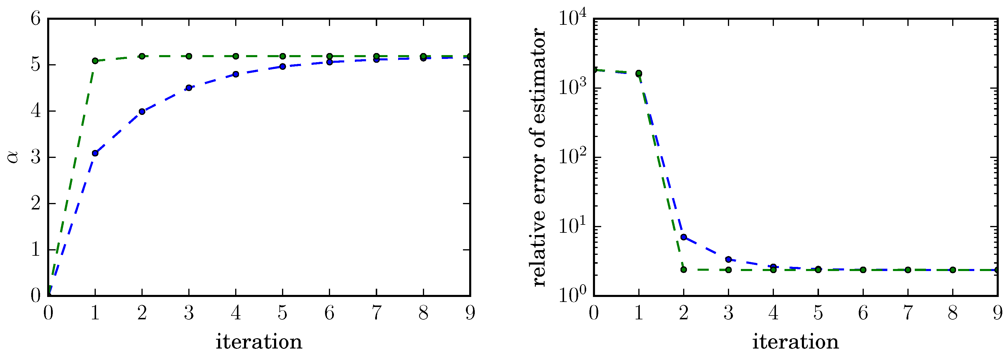
Clearly, the optimal tilting parameter (77) is probably as difficult to compute by brute-force Monte Carlo as the probability $p=P(X>d)$ since $\{X>d\}$ is a rare event when $d\gg 0$ is far away from the mean. The strength of both gradient descent and cross-entropy method is, however, that the optimal tilting parameter can be computed iteratively. This is illustrated numerically in Figure 1 for the choice $d=5$, where we use Algorithm 1 with a constant stepsize and Algorithm 2 as specified. In each iteration m we draw a sample of size $N={10}^8$ from the density ${\rho }^{{\alpha }^{\left(m\right)}}$, and estimate the mean,

$$\widehat{p}=\frac{1}{N}\sum _{i=1}^N{\mathbf{1}}_{\{X_i>d\}}\frac{\pi }{{\rho }^{{\alpha }^{\left(m\right)}}}\left(X_i\right)$$

and the sample variance in each sample. The latter is proportional to the normalized variance $KVar\left(\widehat{p}\right)$ of an estimator that has been estimated K times.

For this (admittedly simple) example both gradient descent and cross-entropy method converge well and lead to a drastic reduction of the normalized relative error $\delta =\sqrt{\mathrm{Var}}\left(\widehat{p}\right)/\widehat{p}$ of the estimator by a factor of about 1000, from about 2000 without importance sampling to about $\delta \approx 2.38$ under (suboptimal) importance sampling with exponential tilting, indicating that both methods can handle situations in which the optimal (i.e., $\delta =0$) change of measure is not available within the set of trial densities.

6. Conclusions

We have presented a method for constructing minimum-variance importance sampling estimators. The method is based on a variational characterization of the thermodynamic free energy and essentially replaces a Monte Carlo sampling problem by a stochastic approximation problem for the optimal importance sampling density. For path sampling, the stochastic approximation problem boils down to a Markov control problem, which again can be solved by stochastic optimization techniques. We have proved that for a large class of path sampling problems that are relevant in, e.g., molecular dynamics or rare events simulation, the (unique) solution to the optimal control problem can yield zero-variance importance sampling schemes.

The computational gain when replacing the sampling problem by a variational principle is, besides improved convergence due to the variance reduction and often a higher hitting rate of the relevant events, due to the fact that the variational problem can be solved iteratively, which makes it amenable to multilevel approaches. The cross-entropy method as an example of such an approach has been presented in some detail. A substantial difficulty still is a clever choice of basis functions that is highly problem-specific, and hence, future research should address non-parametric approaches, as well as model reduction methods in combination with the stochastic optimization/approximation tools that can be used to solve the underlying variational problems.

References

- Hammersely, J.M.; Morton, K.W. Poor Man’s Monte Carlo. J. R. Stat. Soc. Ser. B 1954, 16, 23–38. [Google Scholar]
- Rosenbluth, M.N.; Rosenbluth, A.W. Monte Carlo Calculations of the Average Extension of Molecular Chains. J. Chem. Phys. 1955, 23, 356–359. [Google Scholar] [CrossRef]
- Deuschel, J.D.; Stroock, D.W. Large Deviations; Academic Press: New York, NY, USA, 1989. [Google Scholar]
- Dai Pra, P.; Meneghini, L.; Runggaldier, W.J. Connections between stochastic control and dynamic games. Math. Control Signals Syst. 1996, 9, 303–326. [Google Scholar] [CrossRef]
- Delle Site, L.; Ciccotti, G.; Hartmann, C. Partitioning a macroscopic system into independent subsystems. J. Stat. Mech. Theory Exp. 2017, 2017, 83201. [Google Scholar] [CrossRef]
- Boué, M.; Dupuis, P. A variational representation for certain functionals of Brownian motion. Ann. Probab. 1998, 26, 1641–1659. [Google Scholar]
- Hartmann, C.; Banisch, R.; Sarich, M.; Badowski, T.; Schütte, C. Characterization of rare events in molecular dynamics. Entropy 2014, 16, 350–376. [Google Scholar] [CrossRef]
- Fleming, W.H.; Soner, H.M. Controlled Markov Processes and Viscosity Solutions; Springer: New York, NY, USA, 2006. [Google Scholar]
- Hartmann, C.; Schütte, C. Efficient rare event simulation by optimal nonequilibrium forcing. J. Stat. Mech. Theory Exp. 2012, 2012. [Google Scholar] [CrossRef]
- Jarzynski, C. Nonequilibrium equality for free energy differences. Phys. Rev. Lett. 1997, 78, 2690–2693. [Google Scholar] [CrossRef]
- Sivak, D.A.; Crooks, G.A. Thermodynamic Metrics and Optimal Paths. Phys. Rev. Lett. 2012, 109, 190602. [Google Scholar] [CrossRef] [PubMed]
- Oberhofer, H.; Dellago, C. Optimum bias for fast-switching free energy calculations. Comput. Phys. Commun. 2008, 179, 41–45. [Google Scholar] [CrossRef]
- Rotskoff, G.M.; Crooks, G.E. Optimal control in nonequilibrium systems: Dynamic Riemannian geometry of the Ising model. Phys. Rev. E 2015, 92, 60102. [Google Scholar] [CrossRef] [PubMed]
- Vaikuntanathan, S.; Jarzynski, C. Escorted Free Energy Simulations: Improving Convergence by Reducing Dissipation. Phys. Rev. Lett. 2008, 100, 109601. [Google Scholar] [CrossRef] [PubMed]
- Zhang, W.; Wang, H.; Hartmann, C.; Weber, M.; Schütte, C. Applications of the cross-entropy method to importance sampling and optimal control of diffusions. SIAM J. Sci. Comput. 2014, 36, A2654–A2672. [Google Scholar] [CrossRef]
- Dupuis, P.; Wang, H. Importance sampling, large deviations, and differential games. Stoch. Int. J. Probab. Stoch. Proc. 2004, 76, 481–508. [Google Scholar] [CrossRef]
- Dupuis, P.; Wang, H. Subsolutions of an Isaacs equation and efficient schemes for importance sampling. Math. Oper. Res. 2007, 32, 723–757. [Google Scholar] [CrossRef]
- Vanden-Eijnden, E.; Weare, J. Rare Event Simulation of Small Noise Diffusions. Commun. Pure Appl. Math. 2012, 65, 1770–1803. [Google Scholar] [CrossRef]
- Roberts, G.O.; Tweedie, R.L. Exponential convergence of Langevin distributions and their discrete approximations. Bernoulli 1996, 2, 341–363. [Google Scholar] [CrossRef]
- Glasserman, P. Monte Carlo Methods in Financial Engineering; Springer: New York, NY, USA, 2004. [Google Scholar]
- Lelièvre, T.; Stolz, G. Partial differential equations and stochastic methods in molecular dynamics. Acta Numer. 2016, 25, 681–880. [Google Scholar] [CrossRef]
- Bennett, C.H. Efficient estimation of free energy differences from Monte Carlo data. J. Comput. Phys. 1976, 22, 245–268. [Google Scholar] [CrossRef]
- Øksendal, B. Stochastic Differential Equations: An Introduction with Applications; Springer: Berlin, Germany, 2003. [Google Scholar]
- Lapeyre, B.; Pardoux, E.; Sentis, R. Méthodes de Monte Carlo Pour les Équations de Transport et de Diffusion; Springer: Berlin, Germany, 1998. (In French) [Google Scholar]
- Sivak, D.A.; Chodera, J.D.; Crooks, G.A. Using Nonequilibrium Fluctuation Theorems to Understand and Correct Errors in Equilibrium and Nonequilibrium Simulations of Discrete Langevin Dynamics. Phys. Rev. X 2013, 3, 11007. [Google Scholar] [CrossRef]
- Darve, E.; Rodriguez-Gomez, D.; Pohorille, A. Adaptive biasing force method for scalar and vector free energy calculations. J. Chem. Phys. 2008, 128, 144120. [Google Scholar] [CrossRef] [PubMed]
- Lelièvre, T.; Rousset, M.; Stoltz, G. Computation of free energy profiles with parallel adaptive dynamics. J. Chem. Phys. 2007, 126, 134111. [Google Scholar] [CrossRef] [PubMed]
- Lelièvre, T.; Rousset, M.; Stoltz, G. Long-time convergence of an adaptive biasing force methods. Nonlinearity 2008, 21, 1155–1181. [Google Scholar] [CrossRef]
- Hartmann, C.; Schütte, C.; Zhang, W. Model reduction algorithms for optimal control and importance sampling of diffusions. Nonlinearity 2016, 29, 2298–2326. [Google Scholar] [CrossRef]
- Zhang, W.; Hartmann, C.; Schütte, C. Effective dynamics along given reaction coordinates, and reaction rate theory. Faraday Discuss. 2016, 195, 365–394. [Google Scholar] [CrossRef] [PubMed]
- Hartmann, C.; Latorre, J.C.; Pavliotis, G.A.; Zhang, W. Optimal control of multiscale systems using reduced-order models. J. Comput. Nonlinear Dyn. 2014, 1, 279–306. [Google Scholar] [CrossRef]
- Hartmann, C.; Schütte, C.; Weber, M.; Zhang, W. Importance sampling in path space for diffusion processes with slow-fast variables. Probab. Theory Relat. Fields 2017. [Google Scholar] [CrossRef]
- Lie, H.C. On a Strongly Convex Approximation of a Stochastic Optimal Control Problem for Importance Sampling of Metastable Diffusions. Ph.D. Thesis, Department of Mathematics and Computer Science, Freie Universität Berlin, Berlin, Germany, 2016. [Google Scholar]
- Richter, L. Efficient Statistical Estimation Using Stochastic Control and Optimization. Master’s Thesis, Department of Mathematics and Computer Science, Freie Universität Berlin, Berlin, Germany, 2016. [Google Scholar]
- Nocedal, J.; Wright, S.J. Numerical Optimization; Springer: New York, NY, USA, 1999. [Google Scholar]
- Banisch, R.; Hartmann, C. A sparse Markov chain approximation of LQ-type stochastic control problems. Math. Control Relat. Fields 2016, 6, 363–389. [Google Scholar] [CrossRef]
- Schütte, C.; Winkelmann, S.; Hartmann, C. Optimal control of molecular dynamics using Markov state models. Math. Program. Ser. B 2012, 134, 259–282. [Google Scholar] [CrossRef]
- Bertsekas, D.P. Approximate policy iteration: A survey and some new methods. J. Control Theory Appl. 2011, 9, 310–355. [Google Scholar] [CrossRef] [Green Version]
- El Karoui, N.; Hamadène, S.; Matoussi, A. Backward stochastic differential equations and applications. Appl. Math. Optim. 2008, 27, 267–320. [Google Scholar]
- Bender, C.; Steiner, J. Least-Squares Monte Carlo for BSDEs. In Numerical Methods in Finance; Carmona, R., Del Moral, P., Hu, P., Oudjane, N., Eds.; Springer: Berlin/Heidelberg, Germany, 2012; pp. 257–289. [Google Scholar]
- Gobet, E.; Turkedjiev, P. Adaptive importance sampling in least-squares Monte Carlo algorithms for backward stochastic differential equations. Stoch. Proc. Appl. 2005, 127, 1171–1203. [Google Scholar] [CrossRef]
- Hartmann, C.; Kebiri, O.; Neureither, L. Importance sampling of rare events using least squares Monte Carlo. 2018; under preparation. [Google Scholar]
- Papaspiliopoulos, O.; Roberts, G.O. Importance sampling techniques for estimation of diffusions models. In Centre for Research in Statistical Methodology; Working Papers, No. 28; University of Warwick: Coventry, UK, 2009. [Google Scholar]
Figure 1.
Comparison of the cross-entropy (green) and the gradient descent method (blue) for a rare event with probability for fixed sample size . Both algorithms quickly converge to the optimal tilting parameter for the family of importance sampling distributions (left panel) and lead to a drastic reduction of the normalized relative error by a factor of 1000, from about 2000 to 2.38 after few iterations (right panel).
© 2017 by the authors. Licensee MDPI, Basel, Switzerland. This article is an open access article distributed under the terms and conditions of the Creative Commons Attribution (CC BY) license (http://creativecommons.org/licenses/by/4.0/).
Share and Cite
MDPI and ACS Style
Hartmann, C.; Richter, L.; Schütte, C.; Zhang, W. Variational Characterization of Free Energy: Theory and Algorithms. Entropy 2017, 19, 626. https://doi.org/10.3390/e19110626
AMA Style
Hartmann C, Richter L, Schütte C, Zhang W. Variational Characterization of Free Energy: Theory and Algorithms. Entropy. 2017; 19(11):626. https://doi.org/10.3390/e19110626
Chicago/Turabian StyleHartmann, Carsten, Lorenz Richter, Christof Schütte, and Wei Zhang. 2017. "Variational Characterization of Free Energy: Theory and Algorithms" Entropy 19, no. 11: 626. https://doi.org/10.3390/e19110626
Note that from the first issue of 2016, this journal uses article numbers instead of page numbers. See further details here.