Diagnosis of Combined Cycle Power Plant Based on Thermoeconomic Analysis: A Computer Simulation Study

1
Department of Automobiles, Chosun College of Science and Technology, Gwangju 61453, Korea
2
School of Mechanical Engineering, Chung-Ang University, Seoul 06974, Korea
3
Blue Economy Strategy Institute Co. Ltd., Seoul 06721, Korea
*
Author to whom correspondence should be addressed.
Entropy 2017, 19(12), 643; https://doi.org/10.3390/e19120643
Submission received: 12 September 2017
/
Revised: 16 November 2017
/
Accepted: 25 November 2017
/
Published: 28 November 2017
(This article belongs to the Section Thermodynamics)
Abstract
:In this study, diagnosis of a 300-MW combined cycle power plant under faulty conditions was performed using a thermoeconomic method called modified productive structure analysis. The malfunction and dysfunction, unit cost of irreversibility and lost cost flow rate for each component were calculated for the cases of pre-fixed malfunction and the reference conditions. A commercial simulating software, GateCycleTM (version 6.1.2), was used to estimate the thermodynamic properties under faulty conditions. The relative malfunction (RMF) and the relative difference in the lost cost flow rate between real operation and reference conditions (RDLC) were found to be effective indicators for the identification of faulty components. Simulation results revealed that 0.5% degradation in the isentropic efficiency of air compressor, 2% in gas turbine, 2% in steam turbine and 2% degradation in energy loss in heat exchangers can be identified. Multi-fault scenarios that can be detected by the indicators were also considered. Additional lost exergy due to these types of faulty components, that can be detected by RMF or RDLC, is less than 5% of the exergy lost in the components in the normal condition.
1. Introduction
The performance of a power plant deteriorates during operation due to degradation in plant components. Common causes of degradation in power plants include fouling of heat exchangers in steam generators and corrosion and/or erosion that occurs in compressors and turbine blades. Degradation in a component results in changes in the thermodynamic properties at the entrance/exit points of the components, performance of the components and system and the cost of products of the system. When degradation occurs in a component, it is necessary to perform maintenance of the component to improve the performance of the plant. However, identification of a malfunctioning component is not a simple task when the deviation is less than 3%, which cannot be detected by the operator [1]. Furthermore it is not feasible to detect the components when anomalies occur simultaneously, because the interaction between components is very complex.
Diagnosis of power plants corresponds to the detection of malfunctioning components, identification of the causes of the malfunction, and the quantification of the malfunction [2]. Thermoeconomics, which combines the thermodynamics concept of exergy with economic principle, quantifies the exergy destruction and the corresponding monetary loss occurred at each component in power plants [3]. Such merits of thermoeconomics which quantifies the exergy destruction due to the entropy generation and the corresponding lost cost depending on the degree of malfunction make it possible to apply to diagnosis of energy systems. A possible application of thermoeconomics to diagnose a power system was first suggested by Lozano et al. [4] and Valero et al. [5]. A feasibility of the diagnosis of a power plant based on thermoeconomic analysis was provided by Correas et al. [6]. Further development of the thermoeconomic diagnosis which clarified the intrinsic and induced malfunction and determined the cost generated by the malfunction in degraded components was undertaken by Verda et al. [7,8], Torres et al. [9], and Valero et al. [10]. A characteristic curve method to locate and categorize malfunctions was proposed by Lazzaretto and Toffolo [11] and Toffolo and Lazzaretto [12]. Thermoeconomic diagnosis was applied to evaluate the performance degradation of coal-fired power plants [13]. Recently, two thermoeconomic diagnosis methods were applied to a combined cycle plant [14] and refrigerant system [15,16]. The conventional thermoeconomic diagnosis for air conditioning unit yields promising results for evaporator fouling. However, it does not provide reliable results for condenser fouling [16]. Cziesla and Tsatsaronis [17] performed exergoeconomic assessment of the performance degradation in a coal-fired steam power plant by using the unit cost of product in components as an indicator to identify malfunctioning components. Energy efficiency diagnosis is a mature tool in power plant operation and management at present [18,19]. However, advanced monitoring and diagnosis techniques based on thermoeconomics [20] are required and should be developed.
In the present study, a modified productive structure analysis (MOPSA) [3] method that provides irreversibility due to entropy generation and it allocates a lost cost flow rate for each component was applied to simulate the performance degradation due to the pre-fixed malfunctioning components for a conventional 300-MW combined cycle power plant (CCPP) at 100% load. Thermodynamic properties, such as temperatures, pressures and mass flow rates for the power plant with pre-fixed malfunction components were estimated using the GateCycleTM energy balance software. Multi-fault scenarios that can be detected by the indicators were also considered. The relative malfunction (RMF) and the difference in the lost cost flow rate between real operation and reference conditions (RDLC) were used as indicators for the identification of malfunction components. Calculation results indicate that thermoeconomic diagnosis method presented in this study could allow detecting the faulty components in the plant and evaluate the added cost while the plant is still functional.
2. Cost-Balance Equations for a 300-MW Combined Power Plant
2.1. Modified Productive Structure Analysis (MOPSA) Method [3]
A general exergy-balance equation applicable to any component of thermal systems may be formulated by utilizing the first and second law of thermodynamics [21]. The general exergy-balance equation for the k-th component may be written as:
where and denote the rate of exergy and entropy flows, respectively, in the plant, and in the fifth term denotes the heat transfer interaction between a component and the environment. Assigning a unit exergy cost to every decomposed exergy stream, the cost-balance equation corresponding to the exergy-balance equation for the k-th component is given by [3].
where C denotes the unit cost exergy and CHE, BQ, T, P, W used as the superscripts in Equation (1) and subscripts in Equation (2) denote chemical, steam, thermal, mechanical and work or electricity, respectively. The term includes all financial charges associated with owning and operating the k-th plant component. In this study the steam exergy is decomposed into thermal and mechanical exergies. The exergy costing method based on Equations (1) and (2) is called MOPSA in the sense that these equations yield the productive structure of the thermal systems. The MOPSA method can systematically handle any complex power plant [22,23] and provide the correct unit cost of products for coal-fired power plants [23]. Furthermore, the MOPSA method provides the irreversibility and the lost cost rate due to the entropy production rate in each component in the power plants. Thermal and mechanical exergies and negentropy, play very important roles as internal parameters to calculate the unit cost of various exergies. On the other hand, the MF and DYS method based on the conventional thermoeconomic theory [9] is an upstream analysis of the productive process, which needs difficult and elaborate calculations. Specifically, the total negentropy generated in all components appears as a principal product for the “system boundary”, with a positive sign.
2.2. Levelized Cost of a Plant Component
The costs of owning and operating a plant depend on several factors, including the type of financing, required capital, and expected life of a component. The annualized (levelized) cost method [24] is used in the present study. The amortization cost for a particular plant component is written as follows:
The salvage value at the end of the n-th year is taken as 10% of the initial investment for component Ci. The present worth of the component is converted to the annualized cost by using the capital recovery factor CRF (i,n), as follows:
The levelized cost is divided by 8000 annual operating hours to obtain the following capital cost rate for the k-th component of the plant:
The maintenance cost is considered through the factor for each plant component.
2.3. 300-MW CCPP
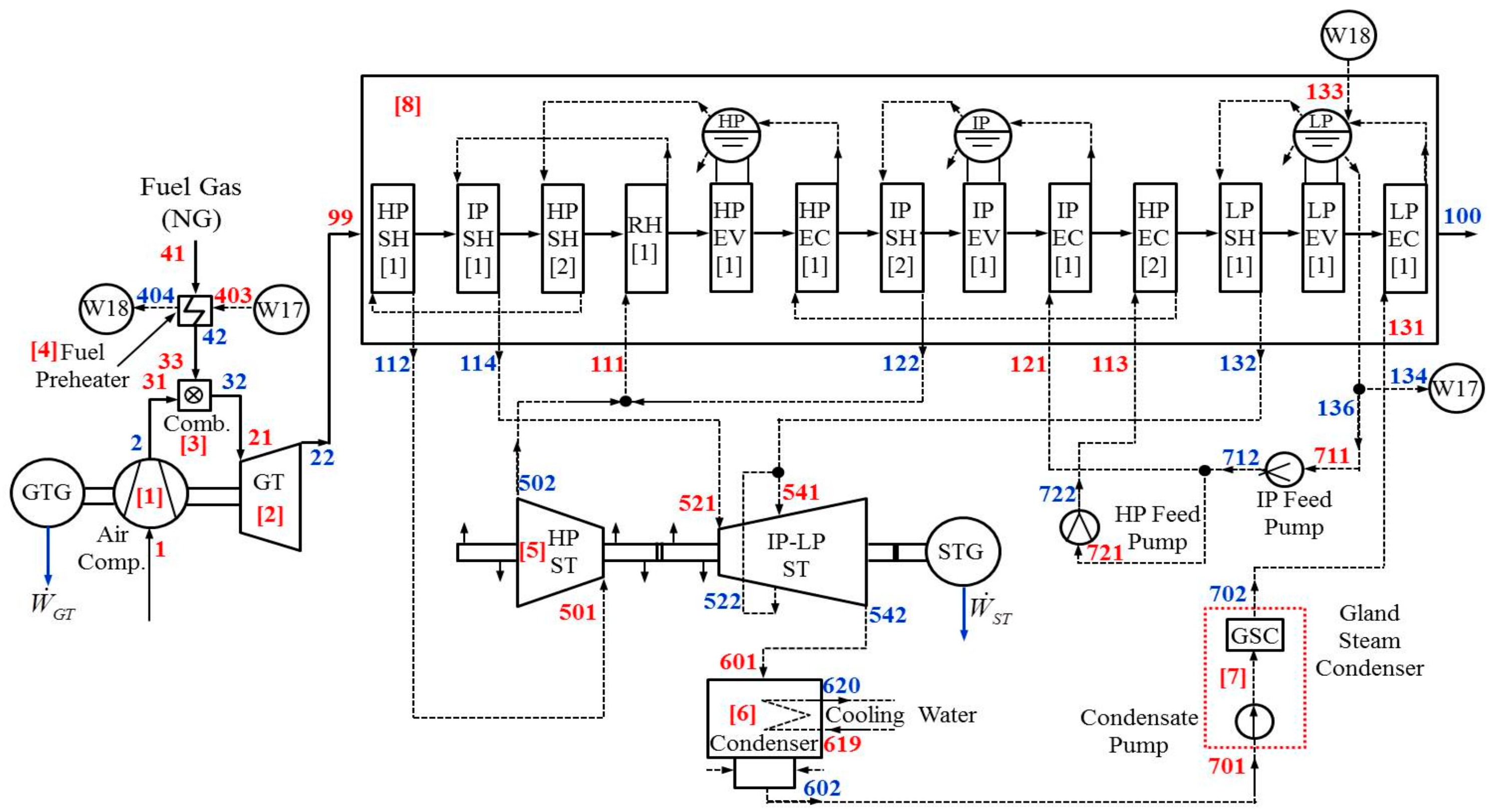
In Figure 1, a schematic representation of a 300-MW CCPP system that is used as a reference plant shows every state point that was accounted for in the analysis. The schematic shows the following eight components: (1) air compressor (AC), (2) gas turbine (GT), (3) combustor (COM), (4) fuel preheater (FP), (5) steam turbine (ST), (6) condenser (CON), (7) pump (PP), and (8) heat recovery steam generator (HRSG). The mass flow rates of fuel, air and steam (or water) and temperature and pressure data at the state points in the 300-MW power plant, which were provided by an electric company in Korea are shown in Table 1. The entropy and thermal and mechanical exergy flow rates were calculated using the data. A detailed calculation was separately performed for the heat exchangers in HRSG by considering the energy loss in the components.
2.4. Cost-Balance Equations for Each Component in a 300-MW CCPP
The cost-balance equations for each component in the CCPP, shown in Figure 1 can be derived from the general cost-balance equation given in Equation (2). A new unit cost must be assigned to the component’s principal product when the cost-balance equation is applied to a component, and its unit cost is expressed as a Gothic letter. For example, an air compressor is a component that uses electricity to increase the mechanical exergy of air. The method assigns a new unit cost of C1P to the mechanical exergy of air, the component’s main product. After the unit cost is assigned to the respective principal product of a component, the cost-balance equations and the corresponding short hand notation for the cost-balance equations for these components are as follows:
- (1)
- Air compressor (AC)
- (2)
- Gas turbine (GT)
- (3)
- Combustor (COM)
- (4)
- Fuel preheater (FP)
- (5)
- Steam turbine (ST)
- (6)
- Condenser (CON)
- (7)
- Pump (PP)
- (8)
- Heat recovery steam generator (HRSG)
- (9)
- Gas pipes
- (10)
- Steam pipes
As shown in Equation (13), the water and steam exergy streams, entering or leaving the HRSG were considered. The heat losses and pressure drops inside pipes in which gases and water or steam flows were considered in Equations (9) and (10), respectively, by assuming that the gas and steam pipes are real components in the system. This concept is necessary for perfect exergy and cost balance of the plant. Ten cost-balance equations from the ten components of the combined plant were derived, with 15 unknown unit exergy costs, namely, C1P, CW, C3T, C4T, DW, C6BQ, D7P, D8T, C9T, D10T, CT, CP, DT, DP and CS. We obtain four more cost-balance equations for the junctions of the thermal and mechanical exergies for gas and steam streams. These four cost-balance equations and the corresponding short-hand notation equations are given as follows:
- (1)
- Gas streams
- (2)
- Steam streams
Another cost-balance equation is obtained, corresponding to the exergy balance for the plant boundary of the combined cycle plant. The cost-balance equation for the system boundary is given as follows:
The overall cost-balance equation is obtained by adding all the cost-balance equations of the components and boundary of the system. The overall cost-balance equation for the plant that may be considered as the first principle in thermoeconomics, is given in previous study [3] as follows:
During the addition of exergy-balance equation of components, the terms related to the unit cost of mechanical energy CP, the thermal exergy CT for gases, the unit cost of mechanical exergy DP, thermal exergy DT for steam, and negentropy CS disappear such that the cost-balance equation for the entire system does not include the aforementioned terms.
The matrix representation of the all cost-balance equations for the CCPP system is shown in Figure 2. Each row in the matrix represents the exergy-balance equation for a component or junction and the diagonal element indicates the principal product for each component. The exergy-balance equation for junction represents a “junction” for the specified exergy. On the other hand, each column in the matrix shows the manner in which an exergy produced in a component (diagonal element) is distributed to or consumed in other components (off diagonal elements). In this sense, the diagonal element in each column represents a “node” in the productive structure for the power plant. For example, the GT interacts with the AC through electricity and mechanical exergy. The thermal exergy produced in the COM and added in the FP () is consumed in the GT to produce electricity () and in the HRSG to increase the exergy of steam (). This implies that a fault that occurred in the GT affects the performance of the AC, COM, FP, and HRSG. The pressure exergy gained in the AC () is consumed in GT () and dissipated in COM () and HRSG (). The lost exergy recovered at the boundary (), which represents the total exergy lost in the system, is distributed among all components (). Subsequently, the total lost cost is allocated to all components in a manner proportional to the amount of the exergy lost. These examples indicate how the components in the plant are related with each other. Summation of all terms in column yields Equation (21), the overall cost-balance equation. As explained above, Figure 2 shows clearly the productive structure of the 300-MW CCPP.
3. Exergy and Thermoeconomic Analyses at a Reference Condition and Identification of Malfunctioning Components
The thermal, mechanical exergy flow rates and entropy flow rates at a reference condition and at 100% load for 300-MW CCPP are shown Table 1. The flow rates were calculated based on the properties such as pressure, temperature, and mass flow rates at various points, which were supplied by a power company. The net flow rates of the various exergies crossing the boundary of each component in the CCPP at the reference condition are shown in Table 2. The unit cost value of fuel, $0.02/MJ, was used in the calculation. Positive values of exergies indicate the exergy flow rate of “products” while negative values represent the exergy flow rate of “resources” or “fuel”. The irreversibility in each component acts as a product in the exergy-balance equation. The sum of the exergy flow rates of products and resources is equal to zero for each component and for the entire plant, and this indicates that perfect exergy balances are satisfied.
The mathematical expression of the exergy-balance for each component, as shown in Equation (1) can be rewritten as follows:
where the superscripts F and P denote fuel and product for i-th component, respectively. For example, each term in Equation (22) in AC is given as follows:
Let ri denote the ratio of the fuel exergy to the product exergy in i-th component, as follows:
Substituting Equation (23) into Equation (22), the irreversibility that occurs at the i-th component can be expressed in terms of the exergy product for the component as follows:
The irreversibility difference between real operation and the reference conditions in the i-th component is expressed as follows [10,25]:
where:
The malfunction (MF) defined in Equation (26) represents the endogenous irreversibility, which is produced by an increase in fuel consumption and the dysfunction (DYS) defined in Equation (27) represents the exogenous irreversibility, which is induced in the component by the malfunction of other components [10]. The MF that does not depend on the mass flow rate of material stream may be selected as one of the indicators to identify the faulty components [10,16]. The DYS is not appropriate for the indicators because the MF only affects the behavior of components [10]. One of the most useful methods to quantify the effects of the intrinsic malfunctions is MF [15]. Previously ΔI and ΔI/I were considered as indicators for evaluation of malfunction in the components [25].
Relative malfunction (RMF) may be defined as the ratio of the MF to the irreversibility that occurs at the reference condition, as follows:
At the very least, the induced malfunction due to the change in the mass flow rate is eliminated in this particular condition. The dysfunction induced by change in the mass flow rate is obtained by the following equation:
where:
The dysfunction modified by eliminating the induced malfunction defined in Equation (29) is as follows:
In fact, the main difficulty in the application of thermoeconomics to the diagnosis of power plant is the presence of the induced malfunctions in the components [19] so that the correct diagnosis consists of successive filtration of the induced effect [26].
Table 3 lists the initial investments, the annuities including the maintenance cost, as well as the corresponding monetary flow rates for each component. The total construction cost that, comprises the cost of land, site preparation, and building construction, are also input into the cost calculation in the “boundary” component. The cost of CO2 emission, which is proportional to carbon content relative to the heating value of fuel spent in the power plant, may be included in fuel cost. The cost flow rates corresponding to a component’s exergy flow rate and the construction cost at the 100% load condition are specified in Table 4. The same sign convention for the cost flow rates related to the products and resources was used as the case of exergy balances shown in Table 2. However, the lost cost flow rate due to the lost work in a component is consumed cost or input cost [27]. Certainly, the lost cost is not a production cost [17]. As shown in Table 4, the sum of the cost flow rates of each component in the plant is zero, and thus the cost balance for each component given in Equation (2) is rewritten as follows:
where the superscripts F and P denote fuel and product for the i-th component, respectively. The lost cost flow rate due to the irreversibility is added as a cost to the component. For example, each term in Equation (31) in AC is given as follows:
The lost cost flow rate encountered in Equation (31) is considered as the cost flow rate of residues [27] if the cost flow rates are proportionally allocated to the entropy generation rate [28]. In the MOPSA method, the same unit cost of negentropy is assigned irrespective of material streams and flow conditions [3].
The difference of the lost cost flow rate between real operation and reference conditions, or the additional lost cost flow rate, can be obtained from Equation (29) by assuming that the capital flow rate for the component does not change. That is expressed as follows:
It is convenient to introduce the relative difference of the lost cost flow rate between real operation and reference conditions (RDLC), which is defined as follows:
The above parameter, RDLC, is utilized as an indicator to identify the malfunctioning component.
The degree of influence on the j-th component due to the fault in the i-th component in terms of the RDLC and MF values is defined as follows:
4. Simulation at Full Load
GateCycleTM energy-balance software developed by GE (Boston, MA, USA) was used to calculate the thermal properties at operating conditions with the pre-fixed malfunctioning component. The thermal properties at the design point at full load were provided by a power company. The performance of the power plant was evaluated in the ISO ambient conditions, namely, 288.15 K and 1.013 bar. The temperature at the combustor outlet was kept constant. The outlet temperature of the COM was kept approximately constant by controlling the mass flow rate of air and fuel. The isentropic efficiency of STs was calculated by using the Spencer, Cotton and Cannon method [29]. The inlet and outlet pressures of pumps (HP feed pump, IP feed pump, and condenser pump) were kept constant with slight variations in the mass flow rates. In all the cases, the net power generated at the power plant was kept approximately constant.
5. Simulation on Performance Degradation for a CCPP
5.1. Thermoeconomic Evaluation of Different Single-Fault Scenarios
If a malfunction occurs at a component in a power plant, then the control system intervenes to restore the desired power output, so that the fuel flow rate, and correspondingly the air flow rate, increase. It is assumed that the capital cost flow rate for the plant and the unit cost of fuel are not changed, and thus the difference in the cost-balance equation for the CCPP between real operation and reference conditions is as follows:
Equation (36) indicates that the increase in the fuel flow rate due to faults in components results in an increase in the unit cost of the products. In the present study, four malfunctions are imposed, either individually or simultaneously: malfunctions in the AC, GT, and steam GT due to corrosion in the blades and malfunction due to fouling in heat exchangers in the HRSG.
First, a case of the air compressor malfunction with 0.5% degraded isentropic efficiency is considered. The exergy balance and the cost balance for each component and entire system at 100% load are shown in Table 5 and Table 6, respectively. In Table 5, the difference in the irreversibility rates between the real operation and reference conditions are also listed. Due to the fault in the air compressor, additional exergy of 595 kW is destructed in the plant and the generated irreversibility is allocated to the AC (448.7 kW), GT (90.5 kW), ST (42.1 kW), HRSG (57.4 kW), and CON (32.5 kW). The calculated RDLC for each component is listed in Table 6. The RDLC in the AC and in GT are 5.14% and 1.51%, respectively. The component that is most affected due to the fault in the AC is the GT which interacts with the AC through electricity such that ξRDLC(AC,GT) = 29.4% and ξMF(AC,GT) = 17.9%. Even though the difference in the irreversibility rate (735 kW) and MF (758 kW) in COM are the largest among the components, the RDLC and RMF values are 0.3% and 0.6%, respectively. It is also noted that the induced irreversibility due to the change in the mass flow rate is very large so that DYS defined in Equation (30) becomes negative and consequently ΔI in COM reduces very much (214.3 kW) as shown in Figure 3.
Table 7 lists the fuel and product exergies for each component at real operation and reference conditions, the ratio of the fuel to the product exergy, the values of MF, DYS, and RMF for the case of 0.5% degraded isentropic efficiency in the air compressor. The RMF value at the air AC approximately corresponds to 4.5%, and it significantly exceeds the values in other components. Hence it is easily identified as a faulty component. Even though the MF value at the COM is the highest among the components, its relative increase (RMF) is rater small. The distributions of the MF and DYS in each component are shown in Figure 3a and the RMF and RDLC are shown in Figure 3b. A significant increase in the lost cost flow rate or additional input cost flow rate occurs in the AC as clearly shown in Figure 3b. A relevant malfunction is accurately detected at the AC, and this indicates that the RMF and RDLC are potentially good indicators to identify the faulty components.
For various cases of faults considered in this study, the mass flow rate, pressure and temperature at key points in the CCPP are listed in Table 8 and the flow rates of fuel exergy, electricity, and irreversibility and the cost flow rates of fuel and electricity are listed in Table 9. Except the cases involving the 2% degradation of isentropic efficiency in the GT, the variation in the flow rates of fuel and the production rate of electricity from the reference condition is small.
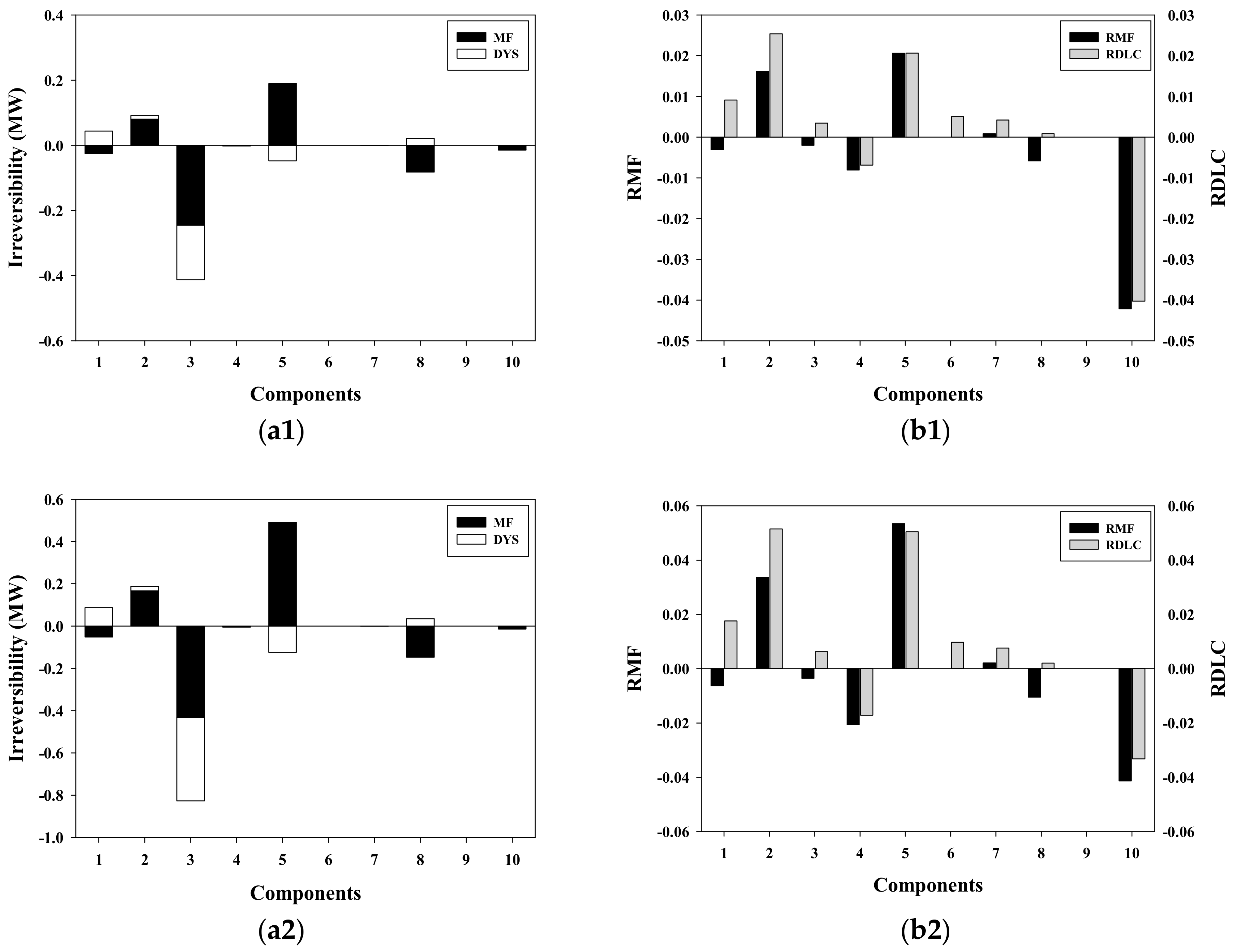
With respect to the case of the 1% degraded isentropic efficiency in the GT, the distributions of the MF and DYS and RMF and RDLC for each component at the 100% load condition are shown in Figure 4 (a1) and (a2), respectively. The MF value and the corresponding RMF value in the GT corresponds to 21.7 kW and 0.44%, respectively due to the fault in the GT. The HRSG with MF and RMF values of 22.6 kW and 0.16%, respectively, is affected by the malfunction of the GT since the HRSG interacts with the GT through thermal exergy. With respect to MF value alone, it is not possible to identify whether the GT is in faulty condition when the irreversibility that occurs in the GT is considerably small. However, the value of the RDLC, which displays the highest value (0.76%) among all the components indicates that malfunction may occur in the GT. In fact, among the additional increase in the lost cost flow rate of 2.925 $/h, a lost cost flow rate of 0.604 $/h only occurs in the GT. A more significant increase in the RDLC (4.3%) at the GT appears when the 2% degradation in the isentropic efficiency in the GT occurs as shown in Figure 4 (b2). The MF and corresponding RMF values increase to 145.2 kW and 2.94%, respectively, if the isentropic efficiency of the GT decreases by 2%. The maximum RMF and RDLC values occur in the GT such that the RMF and RDLC are good indicators to identify a malfunction in the GT. It is noted that the performance of the ST is strongly affected by the malfunction in the GT or, ξRDLC(GT,ST) = 36.4% and ξMF(GT,ST) = 95.5% for the 2% degradation in the isentropic efficiency at the GT.
With respect to the case of the 1% degraded isentropic efficiency in the ST, the distributions of MF and DYS and RMF and RDLC values for each component at the 100% load condition are shown in Figure 5 (a1) and (a2), respectively. The MF and the corresponding RMF are 22.9 kW and 0.25%, respectively, due to the 1% malfunction in the ST. The most affected component due to the fault in the ST is the HRSG in which the MF value corresponds to 23.2 kW such that one can hardly identify whether the ST is in fault condition. Furthermore, the magnitude of RDLC at the HRSG (0.29%) slightly exceeds that at the ST (0.26%) while the RMF value (0.16%) at the HRSG (1.65%) is smaller than the value at ST (0.25%). Evidently, two indicators fail to identify that the fault occurs in the ST when the degradation degree at the ST is excessively small. As shown in Figure 5 (b2), with respect to the case of the 2% degradation in the isentropic efficiency in the ST, the RMF value of 1.34% and the RDLC value of 1.33% allow the detection of the malfunction in the ST, in which an additional exergy of 122.8 kW is lost. The MF value at the ST with the 2% degradation increases to 122.6 kW. The effect of the degradation of the ST on the performance of the GT is rather small, or ξMF(ST,GT) = 13.1%.
A case of fault is considered in one of the heat exchangers in HRSG with 2% degradation efficiency in the HPSH (1). Evidently two indicators, RMF and RDLC suggest that the fault occurs in the HPSH (1), and this appears at the HRSG in Figure 6. The additional exergy (156 kW) that is lost in the HPSH (1) corresponds to a RMF value of 1.05% and the RDLC value that appears at the HRSG approximately corresponds to 1.11%.
5.2. Thermoeconomic Evaluation of Multiple-Fault Scenarios
Simultaneous pre-fixed faults in the AC and GT are considered. With respect to the 0.5% degraded isentropic efficiency in the AC and the 1% degraded isentropic efficiency in the GT, the MF and DYS and RMF and RDLC distributions for each component are shown in Figure 7a,b, respectively. Evidently, the RMF and RDLC values indicate that faults occur both in the AC (4.19% and 5.82%) and GT (2.63% and 3.48%). When the fault occurs in both the AC and GT, the components affect each other to increase the RDLC values in these components. For example, the RDLC value of AC and GT corresponds to 5.14%, and 0.8%, respectively, when a 0.5% degradation in the AC and 1% degradation in the GT independently occur. The faults at both the AC and GT, that are detected by RMF or RDLC values, decrease performance in the ST, or ξRDLC(AC,ST) = 25.9% and ξMF(GT,ST) = 68.4%.
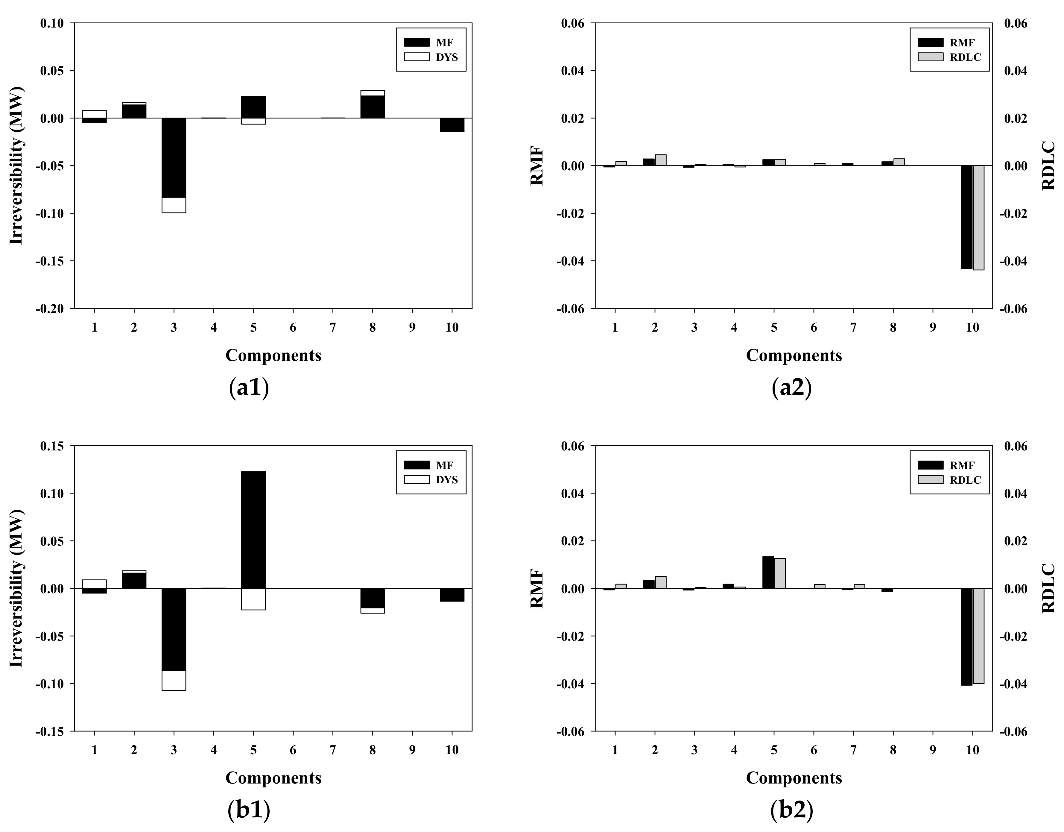
With respect to 1% degraded isentropic efficiency in the GT and 2% in the ST, the distributions of the MF/DYS and RMF/RDLC in the components are shown in Figure 8 (a1) and (b1), respectively. If faults occur both in the GT and ST, then the MF values correspond to 80.2 kW at GT and 189.2 kW at ST. The RMF and RDLC values are 1.62% and 2.54%, respectively, at GT and 2.06% and 2.07%, respectively, at ST. When the degree of the malfunction is doubled at GT and ST, as shown in Figure 8 (a2), the MF values increase to 166.3 kW and 491.5 kW, respectively. The corresponding RMF and RDLC values correspond to 3.4% and 5.15%, respectively at GT and 5.4% and 5.1%, respectively, at ST. The degradation in both GT and ST affects the behavior of AC, or ξRDLC(GT,AC) = 34.1% and ξRDLC(ST,AC) = 34.0%.
With respect to the 0.5% degraded isentropic efficiency in AC, 1% in the GT and 2% in the high-pressure ST, the distributions of the MF and DYS and RMF and RDLC in the components are shown in Figure 9a,b, respectively. The MF values at AC, GT and ST correspond to 338.3 kW, 146.7 kW, and 213.1 kW, respectively, and the values significantly exceed the MF value with a single fault for the cases corresponding to the 1% degradation of GT (21.7 kW) and 2% degradation of ST (122.6 kW). The RMF values at AC, GT, and ST correspond to 4.1%, 3.0% and 2.3%, respectively, while the RDLC values at AC, GT, and ST correspond to 6.6%, 4.0% and 2.2%, respectively. The higher values of MF and appropriate values of RMF and RDLC allow for the identification of faults in these components.
Finally, it is noted that every malfunction at any component produces a favorable effect on the steam pipes, which might be due to more heat exchange between hot water or steam and flue gases. On the other hand the heat exchange in gas pipes is negligible.
5.3. Data during Operation Obtained at Two Months after Major Maintenance
The thermal, mechanical exergy flow rates and entropy flow rates at 100% load which were obtained during the operation two months after a major maintenance are shown in Table 10. The net flow rates of the various exergies crossing the boundary of each component, based on the measured data listed in Table 10 are shown in Table 11. The cost flow rates corresponding to a component’s exergy flow rate are specified in Table 12. In this particular operational condition, less electricity (360.9 MW) from the GT and more electricity (80.1 MW) from ST are produced compared to the values at reference condition. Hence, the increase in the mass flow rates yields more irreversibility in the STs and Steam pipes. In fact, as shown in Table 11 and Figure 10a, significant increase in the additional irreversibility occurs at the GT (3.42 MW), ST (7.61 MW), HRSG (3.83 MW) and Steam pipes (3.43 MW). The RDLC values at GT, ST, HRSG, and Steam pipes correspond to 80.1%, 94.6%, 35.4%, and 1125%, respectively. The higher values of MF at the GT (3.72 MW), ST (7.24 MW), HRSG (3.10 MW), Steam pipes (0.50 MW) and considerably large values of RDLC, as confirmed in Table 11 and Table 12, and Figure 10 indicate that another maintenance should be done near future. In fact, one of engineers in the power company informed us that the efficiencies of STs and heat exchangers in HRSG deteriorated considerably after two or three months of operation.
6. Conclusions
In this study, diagnosis of a 300-MW combined cycle power plant with thermodynamic property data at reference point and during operation was investigated by a computer simulation using the MOPSA method. With help of a commercial simulator, GateCycleTM, the thermodynamic properties at every state point in the plant were estimated under prefixed malfunction conditions. Thermoeconomic diagnosis based on the MOPSA method was applied to single and multiple-fault scenarios. The analysis of four single-fault scenarios in the air compressor, gas turbine, steam turbine and heat exchanger in the steam generator allows detecting and isolating the fault in each component. Multiple-fault scenarios such as simultaneous faults in the air compressor and gas turbine, in the gas turbine and steam turbine and in air compressor, gas turbine and steam turbine were effectively handled by the thermoeconomic diagnosis presented in this study. Real-time diagnosis for the plant was also performed using the thermodynamic data obtained during the operation of the plant. The relative malfunction (RMF) and the difference in the lost cost flow rate between the real operation and reference conditions (RDLC), which show similar response to the degree of fault condition, are found to be good indicators for the identification of faulty components. Simulation results revealed that 0.5% degradation in the isentropic efficiency of air compressor, 2% in gas turbine, 2% in steam turbine and 2% degradation in energy loss in heat exchangers can be identified. The value of MF and the distribution patterns of RMF and RDLC can potentially help in identifying faulty components. This study reveals that the diagnosis of power plants based on MOPSA method may provide a reliable technique for the early identification of faulty components if the thermodynamic data for the plant is monitored.
Author Contributions
Hoo-Suk Oh and Ho-Young Kwak conceived and designed the analysis; Ho-Young Kwak created models; Hoo-Suk Oh performed the calculations; Ho-Young Kwak, Hoo-Suk Oh and Youngseog analyzed the data; Ho-Young Kwak and Youngseog Lee wrote the paper. Authorship must be limited to those who have contributed substantially to the work reported.
Conflicts of Interest
The authors declare no conflict of interest.
Nomenclature
| AC | Air compressor |
| Ci | Initial investment cost (US$) |
| Co | Unit cost of exergy of fuel (US$/kJ) |
| Cs,ref | Unit cost of exergy of fuel at design point (US$/kJ) |
| Cs,op | Unit cost of exergy of fuel at off-design point (US$/kJ) |
| Cw | Unit cost of exergy of work (or electricity) (US$/kJ) |
| Monetary flow rate (US$/year or US$/h) | |
| CCPP | Combined cycle power plant |
| COM | Combustor |
| CON | Condenser |
| CRF | Capital recovery factor |
| D | Unit cost of production for steam (US$/MJ) |
| DYS | Dysfunction |
| Rate of exergy flow (MW) | |
| FP | Fuel preheater |
| GT | Gas turbine |
| HRSG | Heat recovery steam generator |
| Irreversibility rate (MW or kW) | |
| Mass flow rate (kg/s) | |
| MF | Malfunction (kW) |
| MOPSA | Modified productive structure analysis |
| P | Pressure |
| PP | Pump |
| PW | Present worth |
| PWF | Present worth factor |
| Heat transfer rate (MW or kW) | |
| RDLC | Relative difference in the lost cost flow rate between real operation and reference condition |
| RMF | Relative MF value |
| Entropy flow rate (MW/K) | |
| ST | Steam turbine |
| T | Temperature (K) |
| T0 | Ambient temperature (K) |
| Work flow rate | |
| Capital cost rate of unit k (US$/hr) |
Subscripts
| boun | Boundary system |
| cv | Control system |
| k | kth component |
| op | Operational condition |
| P | Mechanical |
| ref | Reference condition |
| S | Entropy |
| T | Thermal |
| W | Work or electricity |
| GS | Gas streams |
| SS | Steam streams |
Superscripts
| BQ | Steam |
| CHE | Chemical |
| F | Fuel |
| LOST | Entropy generation |
| P | Mechanical, production |
| S | Entropy |
| T | Thermal |
| W | Work or electricity |
| WG | Electricity produced by gas turbine |
| WS | Electricity produced by steam turbine |
References
- Gay, R.; MacFarland, M. Model-based performance monitoring and optimization. In Proceedings of the Sixth IFIP/IEEE International Symposium on Integrated Network Management Distributed Management for the Networked Millennium, Boston, MA, USA, 24–28 May 1999. [Google Scholar]
- Valero, A.; Correas, L.; Zaleta, A.; Lazzaretto, A.; Verda, V.; Reini, M.; Rangel, V. On the thermoeconomic approach to the diagnosis of energy system malfunctions Part 1: The TADEUS problem. Energy 2004, 29, 1875–1887. [Google Scholar] [CrossRef]
- Kwak, H.; Kim, D.; Jeon, J. Exergetic and thermoeconomic analyses of power plants. Energy 2003, 28, 343–360. [Google Scholar] [CrossRef]
- Lozano, M.A.; Bartolome, J.L.; Valero, A.; Reini, M. Thermoeconomic diagnosis of energy systems. In Proceedings of the FLOWERS’ 94: Florence World Energy Research Symposium, Florence, Italy, 6–8 July 1994. [Google Scholar]
- Valero, A.; Lozano, M.A.; Bartolome, J.L. On-line monitoring of power-plant performance, using exergetic cost techniques. Appl. Therm. Eng. 1996, 16, 933–948. [Google Scholar] [CrossRef]
- Correas, L.; Martinez, A.; Valero, A. Operation diagnosis of a combined cycle based on the structural theory of thermoeconomics. In Proceedings of the ASME Advanced Energy Systems Division; American Society of Mechanical Engineers: New York, NY, USA, 1999; pp. 381–388. [Google Scholar]
- Verda, V.; Serra, L.; Valero, A. Thermodynamic diagnosis: Zooming strategy applied to highly complex energy systems. Part 1: Detection and localization anomalies. J. Energy Resour. Technol. 2005, 27, 42–49. [Google Scholar] [CrossRef]
- Verda, V.; Serra, L.; Valero, A. Thermoeconomic diagnosis: Zooming strategy applied to highly complex energy systems. Part 2: On the choice of the productive structure. J. Energy Resour. Technol. 2005, 27, 50–58. [Google Scholar] [CrossRef]
- Torres, C.; Valero, A.; Serra, L.; Royo, J. Structural theory and thermodynamic diagnosis, Part 1. On malfunction and dysfunction analysis. Energy Convers. Manag. 2002, 43, 1503–1518. [Google Scholar] [CrossRef]
- Valero, A.; Correas, L.; Zaleta, A.; Lazzaretto, A.; Verda, V.; Reini, M.; Rangel, V. On the thermoeconomic approach to the diagnosis of energy system malfunctions. Part 2. Malfunction definitions and assessment. Energy 2004, 29, 1889–1907. [Google Scholar] [CrossRef]
- Lazzaretto, A.; Toffolo, A. A critical review of the thermoeconomic diagnosis methodologies for the location of causes of malfunctions in energy systems. J. Energy Resour. Technol. 2006, 128, 335–341. [Google Scholar] [CrossRef]
- Lazzaretto, A.; Toffolo, A. A new thermoeconomic method for the location of causes of malfunctions in energy systems. J. Energy Resour. Technol. 2007, 129. [Google Scholar] [CrossRef]
- Valero, A.; Lerch, F.; Serra, L.; Royo, J. Structural theory and thermoeconomic diagnosis. Part II: Application to an actual power plant. Energy Convers. Manag. 2002, 43, 1519–1535. [Google Scholar] [CrossRef]
- Lazzaretto, A.; Toffolo, A.; Reini, M.; Taccani, R.; Zaleta-Aguilar, A.; Rangel-Hernandez, V.; Verda, V. Four approaches compared on the TADEUS (thermoeconomic approach to the diagnosis of energy utility systems) test case. Energy 2006, 31, 1586–1613. [Google Scholar] [CrossRef]
- Ommen, T.; Sigthorsson, O.; Elmegaard, B. Two thermoeconomic diagnosis method applied to representative operating data of a commertial transcrital refrigeration plant. Entropy 2017, 19, 69. [Google Scholar] [CrossRef]
- Piacenttino, A.; Talamo, M. Critical analysis of conventional thermoeconomic approaches to the diagnosis of multiple fault in air conditioning units: Capabilities, drawbacks and improvement directions. A case study for an air-cooled system with 120 kW capacity. Int. J. Refrig. 2013, 36, 24–44. [Google Scholar] [CrossRef]
- Cziesla, F.; Tsatsaronis, G. Exergoeconomic assessment of the performance degradation in a power plant at full and partial load. In Proceedings of the 2003 ASME International Mechanical Engineering Congress, Washington, DC, USA, 15–21 November 2003. [Google Scholar]
- Kim, S.M.; Joo, Y. Implementation of on-line performance monitoring system at Seoincheon and Sinincheon combined cycle plant. Energy 2005, 30, 2383–2401. [Google Scholar] [CrossRef]
- Usón, S.; Valero, A.; Correas, L. Energy efficiency assessment and improvement in energy intensive systems through thermoeconomic diagnosis of the operation. Appl. Energy 2010, 87, 1989–1995. [Google Scholar] [CrossRef]
- Ozgener, L.; Ozgener, O. Monetering of energy exergy efficiencies and exergoeconomic parameters of geothermal district heating systems (GDHSs). Appl. Energy 2009, 86, 1704–1711. [Google Scholar] [CrossRef]
- Oh, S.; Bang, H.; Kim, S.; Kwak, H. Exergy analysis for a gas turbine cogeneration system. J. Eng. Gas Turbine Power 1996, 118, 782–791. [Google Scholar] [CrossRef]
- Kim, D.; Kim, J.H.; Barry, K.F.; Kwak, H. Thermoeconomic analysis of high-temperature gas-cooled reactors with steam methane reforming for hydrogen production. Nucl. Technol. 2011, 176, 337–351. [Google Scholar] [CrossRef]
- Uysal, C.; Kurt, H.; Kwak, H. Exergetic and thermoeconomic analyses of a coal-fired power plant. Int. J. Therm. Sci. 2017, 117, 106–120. [Google Scholar] [CrossRef]
- Moran, J. Availability Analysis: A Guide to Efficient Energy Use; Prentice-Hill: Englewood Cliffs, NJ, USA, 1982. [Google Scholar]
- Toffolo, A.; Lazzaretto, A. On the thermoeconomic approach to the diagnosis of energy system malfunction. Int. J. Thermodyn. 2004, 7, 41–49. [Google Scholar]
- Verda, V.; Borchiellini, R. Exergy method for the diagnosis of energy systems using measured data. Energy 2007, 32, 490–498. [Google Scholar] [CrossRef]
- Torres, C.; Varelo, A.; Rangel, V.; Zaleta, A. On the cost formation process of the residues. Energy 2008, 33, 144–152. [Google Scholar] [CrossRef]
- Lozano, M.A.; Valero, A. Thermoeconomic analysis of a gas turbine cogeneration system. In Thermodynamics and the Design, Analysis, and Improvement of Energy Systems; American Society of Mechanical Engineers: New York, NY, USA, 1993; Volume 30, pp. 312–320. [Google Scholar]
- Cotton, K. Evaluating and Improving Steam Turbine Performance; Cotton Fact Inc.: Rexford, NY, USA, 1998. [Google Scholar]
Figure 1.
300-MW CCPP in Incheon, Korea.

Figure 2.
Cost structure for the 300-MW CCPP.
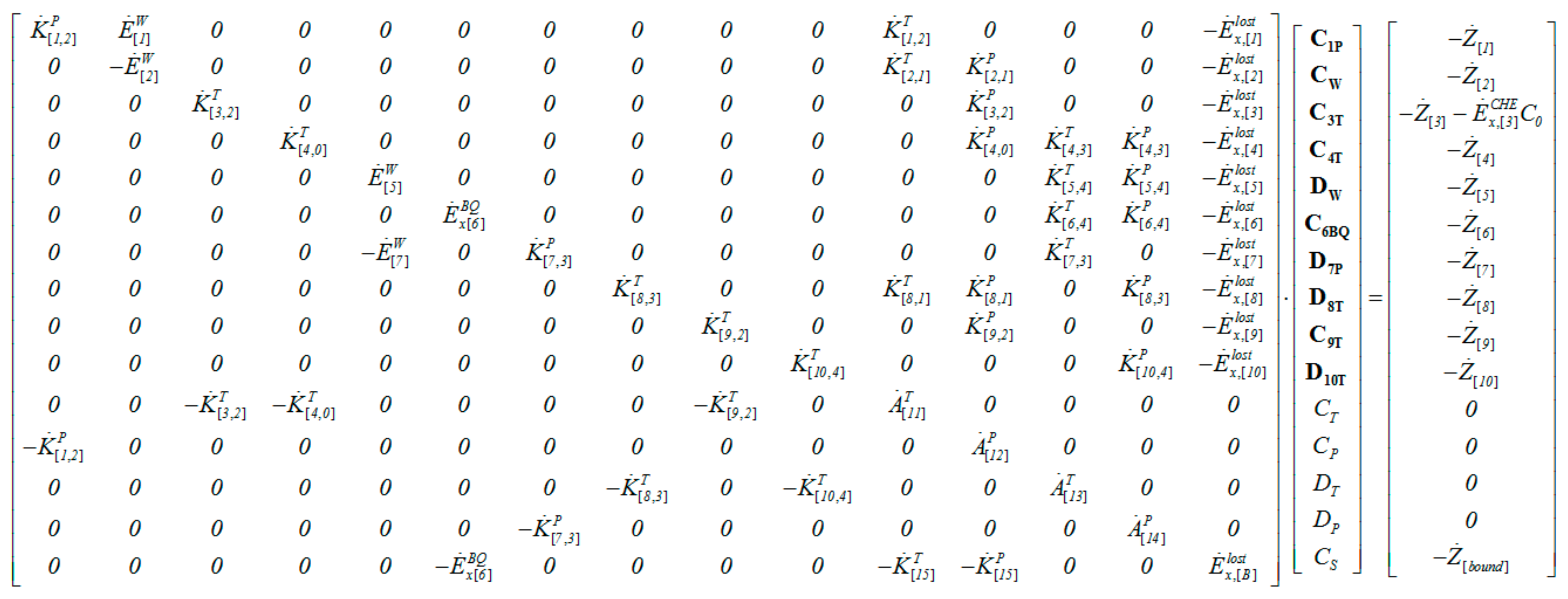
Figure 3.
Distributions of MF and DYS (a) and RMF and RDLC (b) for components of the CCPP with the 0.5% degraded isentropic efficiency in the air compressor at 100% load condition.
Figure 3.
Distributions of MF and DYS (a) and RMF and RDLC (b) for components of the CCPP with the 0.5% degraded isentropic efficiency in the air compressor at 100% load condition.
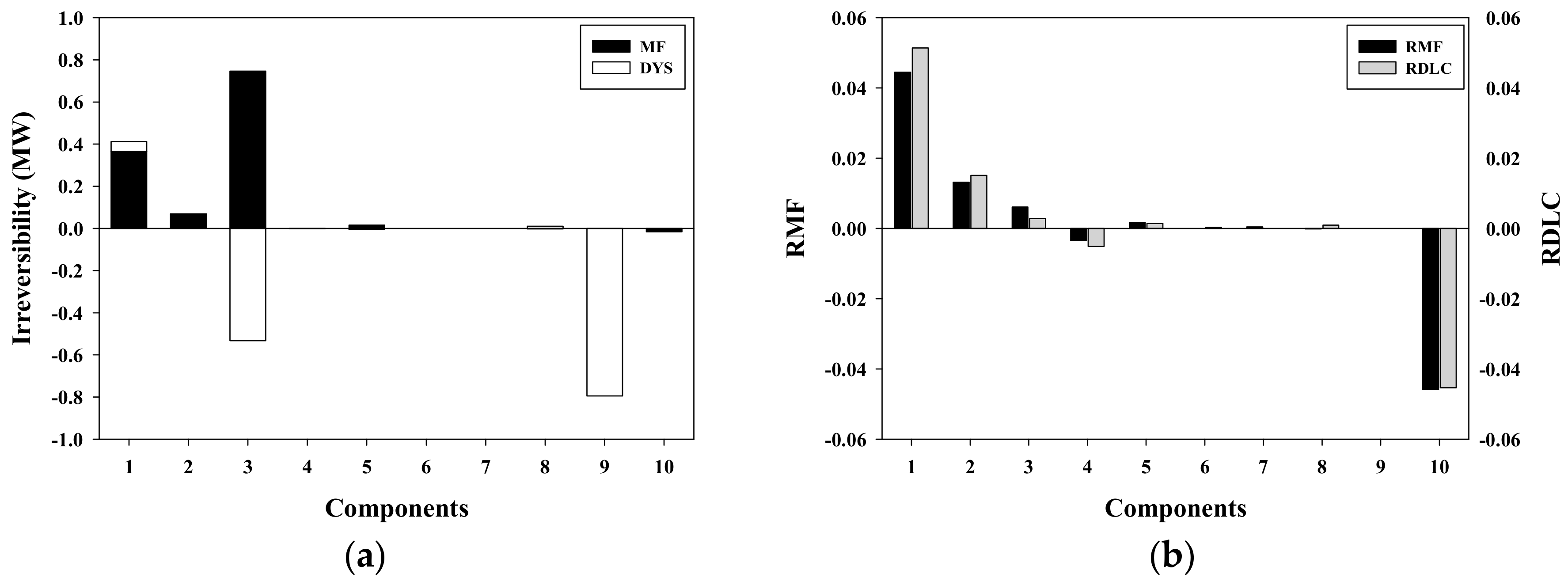
Figure 4.
Distributions of MF and DYS (a1,b1) and RMF and RDLC (a2,b2) for components of the CCPP with the 1% (a1,a2) and 2% (b1,b2) degraded isentropic efficiency in the gas turbine at 100% load condition.
Figure 4.
Distributions of MF and DYS (a1,b1) and RMF and RDLC (a2,b2) for components of the CCPP with the 1% (a1,a2) and 2% (b1,b2) degraded isentropic efficiency in the gas turbine at 100% load condition.

Figure 5.
Distributions of MF and DYS (a1,b1) and RMF and RDLC (a2,b2) for components of the CCPP with the 1% (a1,a2) and 2% (b1,b2) degraded isentropic efficiency in the steam turbine at 100% load condition.
Figure 5.
Distributions of MF and DYS (a1,b1) and RMF and RDLC (a2,b2) for components of the CCPP with the 1% (a1,a2) and 2% (b1,b2) degraded isentropic efficiency in the steam turbine at 100% load condition.

Figure 6.
Distributions of MF and DYS (a) and RMF and RDLC (b) for components of the CCPP with the 2% degraded efficiency in the HPSH (1) at 100% load condition.
Figure 6.
Distributions of MF and DYS (a) and RMF and RDLC (b) for components of the CCPP with the 2% degraded efficiency in the HPSH (1) at 100% load condition.
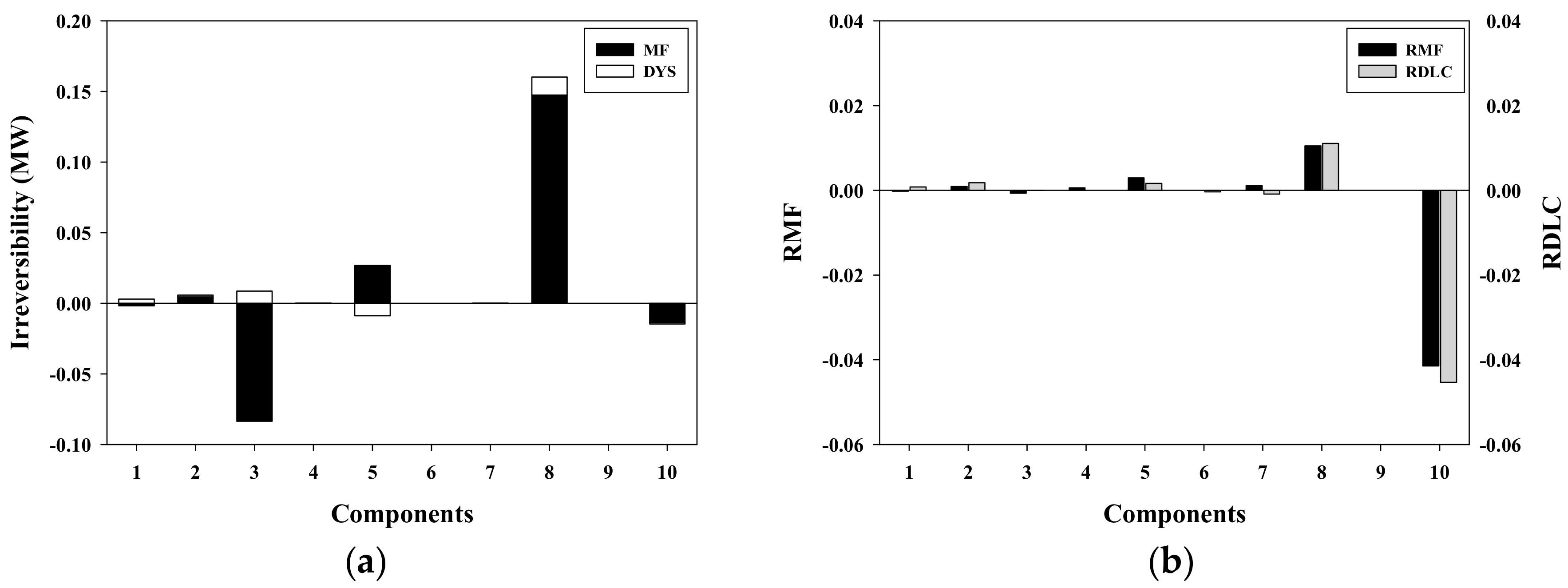
Figure 7.
Distributions of MF and DYS (a) and RMF and RDLC (b) for components of the CCPP with the 0.5% degraded efficiency in the air compressor and 1% in the gas turbine at 100% load condition.
Figure 7.
Distributions of MF and DYS (a) and RMF and RDLC (b) for components of the CCPP with the 0.5% degraded efficiency in the air compressor and 1% in the gas turbine at 100% load condition.
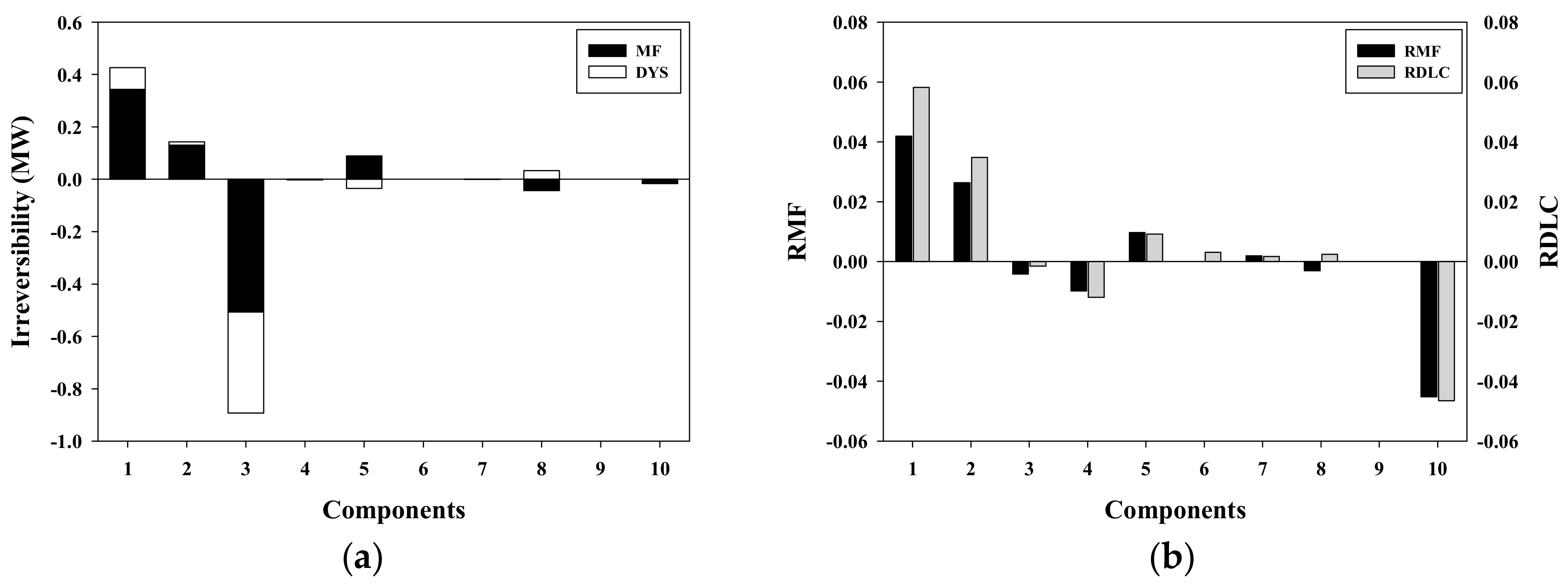
Figure 8.
Distributions of MF and DYS (a1,a2) and RMF and RDLC (b1,b2) for components of the CCPP with the 1% degraded isentropic efficiency in the gas turbine and 2% degraded efficiency in steam turbine (a1,b1) and with the 2% degraded isentropic efficiency in the gas turbine and the 4% degraded efficiency in steam turbine (a2,b2) at 100% load condition.

Figure 9.
Distributions of MF and DYS (a) and RDLC (b) for components of the CCPP with the 0.5% degraded efficiency in the air compressor, 1% in the gas turbine, and 2% in the steam turbine at 100% load condition.
Figure 9.
Distributions of MF and DYS (a) and RDLC (b) for components of the CCPP with the 0.5% degraded efficiency in the air compressor, 1% in the gas turbine, and 2% in the steam turbine at 100% load condition.
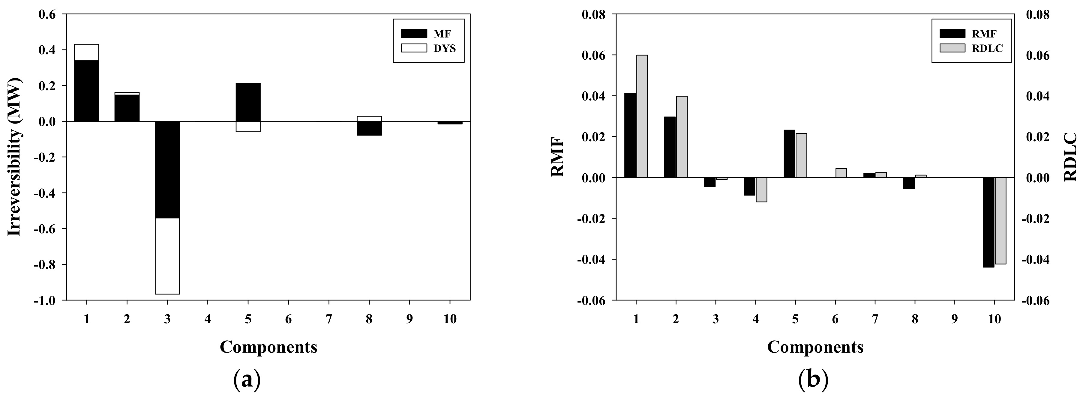
Figure 10.
Distributions of MF and DYS (a) and RDLC (b) for components of the CCPP during operation two months after a major maintenance.
Figure 10.
Distributions of MF and DYS (a) and RDLC (b) for components of the CCPP during operation two months after a major maintenance.


Table 1.
Property values, entropy production rates, and thermal and mechanical exergy flows at various state points in the CCPP at 100% load condition.
Table 1.
Property values, entropy production rates, and thermal and mechanical exergy flows at various state points in the CCPP at 100% load condition.
| States | (ton/h) | P (Mpa) | T (°C) | S (kJ/kg-K) | (kJ/kg) | (kJ/kg) |
|---|---|---|---|---|---|---|
| 1 | 1565.111 | 0.1033 | 15.000 | 0.1366 | 0.000 | 0.0161 |
| 2 | 1565.111 | 1.6099 | 388.9335 | 0.2020 | 139.7690 | 228.1459 |
| 21 | 1597.340 | 1.5536 | 1235.976 | 1.2912 | 883.9721 | 228.3680 |
| 22 | 1597.340 | 0.1071 | 546.8433 | 1.3299 | 255.7211 | 3.0750 |
| 31 | 1565.111 | 1.6099 | 388.9335 | 0.2020 | 139.7690 | 228.1459 |
| 32 | 1597.340 | 1.5536 | 1235.976 | 1.2912 | 883.9721 | 228.3680 |
| 33 | 32.229 | 2.8128 | 110.000 | −0.9940 | 29.5701 | 429.3575 |
| 41 | 32.229 | 2.8128 | 21.111 | −1.6042 | 0.1362 | 422.8056 |
| 42 | 32.229 | 2.8128 | 110.000 | −0.9940 | 29.5701 | 429.3575 |
| 99 | 1597.340 | 0.1071 | 546.8433 | 1.3299 | 255.7211 | 3.0750 |
| 100 | 1597.340 | 0.1033 | 93.3225 | 0.4572 | 9.4904 | 0.0245 |
| 111 | 197.203 | 1.7577 | 292.0264 | 6.8060 | 1052.3238 | 1.6550 |
| 112 | 140.813 | 10.3267 | 537.778 | 6.7013 | 1526.5190 | 10.2075 |
| 113 | 140.813 | 10.8976 | 117.6855 | 1.4931 | 62.0872 | 10.7761 |
| 114 | 197.203 | 1.6874 | 518.5048 | 7.5658 | 1331.1685 | 1.5847 |
| 121 | 56.390 | 1.9715 | 116.3201 | 1.4861 | 60.8700 | 1.8689 |
| 122 | 56.390 | 1.7577 | 271.9138 | 6.7210 | 1029.6400 | 1.6551 |
| 131 | 225.284 | 0.3164 | 33.0516 | 0.4783 | 2.2686 | 0.2132 |
| 132 | 27.856 | 0.1687 | 165.2006 | 7.4341 | 661.2790 | 0.0655 |
| 133 | 19.000 | 4.8340 | 55.000 | 0.7650 | 10.6010 | 4.7290 |
| 134 | 19.000 | 4.9210 | 152.900 | 1.8661 | 106.4457 | 4.8161 |
| 136 | 197.203 | 0.1758 | 115.5952 | 1.4798 | 60.1326 | 0.0725 |
| 403 | 19.000 | 4.9210 | 150.900 | 1.8460 | 103.6750 | 4.8160 |
| 404 | 19.000 | 4.8340 | 55.000 | 0.7650 | 10.6010 | 4.7290 |
| 501 | 140.813 | 10.3267 | 537.7778 | 6.7013 | 1526.5187 | 10.2075 |
| 502 | 140.813 | 1.7577 | 300.2474 | 6.8392 | 1061.6510 | 1.6551 |
| 521 | 197.203 | 1.6874 | 518.5048 | 7.5658 | 1331.1685 | 1.5847 |
| 522 | 197.203 | 0.1758 | 228.0304 | 7.6842 | 715.2606 | 0.0725 |
| 541 | 225.059 | 0.1687 | 220.118 | 7.6716 | 703.3274 | 0.0655 |
| 542 | 225.059 | 0.0051 | −0.950 | 7.9916 | 140.1875 | −0.0983 |
| 601 | 225.059 | 0.0051 | −0.950 | 7.9916 | 140.1875 | −0.0983 |
| 602 | 225.2794 | 0.0051 | 33.0154 | 0.4779 | 2.2601 | −0.0983 |
| 603 | 0.225 | 0.1055 | 15.5556 | 0.2324 | 0.0022 | 0.0022 |
| 619 | 18,106.420 | 0.2110 | 10.000 | 0.1510 | 0.1839 | 0.1078 |
| 620 | 18,106.420 | 0.2110 | 16.800 | 0.2504 | 0.0234 | 0.1078 |
| 701 | 225.284 | 0.0051 | 33.0154 | 0.4779 | 2.2601 | −0.0983 |
| 702 | 225.284 | 0.3164 | 33.0516 | 0.4783 | 2.2686 | 0.2132 |
| 711 | 56.390 | 0.1758 | 115.5953 | 1.4798 | 60.1327 | 0.0725 |
| 712 | 56.390 | 1.9715 | 116.3201 | 1.4861 | 60.8700 | 1.8689 |
| 721 | 140.813 | 1.9715 | 116.3201 | 1.4861 | 60.8700 | 1.8689 |
| 722 | 140.813 | 10.8976 | 117.6855 | 1.4931 | 62.0872 | 10.7761 |
Table 2.
Exergy balances of each component in the CCPP at 100% load condition.
| Component | Net Exergy Flow Rate (MW) | Irreversibility Rate (MW) | |||
|---|---|---|---|---|---|
| Air Compressor | −168.1440 | 0.0000 | 60.7650 | 99.1801 | 8.1991 |
| Gas turbine | 373.7762 | 0.0000 | −278.7580 | −99.9638 | 4.9460 |
| Combustor | 0.0000 | −452.0920 | 331.1936 | −1.7028 | 122.6009 |
| Fuel preheater | 0.0000 | 0.0000 | −0.2277 | 0.0582 | 0.1695 |
| Steam turbine | 78.3664 | 0.0000 | −87.1272 | −0.4276 | 9.1884 |
| Condenser | 0.0000 | 0.0000 | −9.4296 | 0.0000 | 9.4296 |
| Pump | −0.5699 | 0.0000 | 0.0597 | 0.3960 | 0.1142 |
| HRSG | 0.0000 | 0.0000 | −12.6930 | −1.3664 | 14.0678 |
| Gas pipe | 0.0000 | 0.0000 | 0.0000 | 0.0000 | 0.0000 |
| Steam pipes | 0.0000 | 0.0000 | −0.3796 | 0.0449 | 0.3263 |
| Total | 283.4284 | −452.0920 | 3.4027 | −3.7813 | 169.0418 |
Table 3.
Initial investments, annualized costs and corresponding monetary flow rates of each component in the CCPP.
Table 3.
Initial investments, annualized costs and corresponding monetary flow rates of each component in the CCPP.
| Component | Initial Investment Cost | Annualized Cost | Monetary Flow Rate |
|---|---|---|---|
| ($106) | (×$103/year) | ($/h) | |
| Compressor | 20.032 | 2571.634 | 340.609 |
| Combustor | 1.175 | 150.784 | 19.979 |
| Gas turbine | 15.827 | 2031.022 | 269.110 |
| Fuel preheater | 4.056 | 520.492 | 68.965 |
| HRSG | 0.015 | 1.951 | 0.258 |
| Steam turbine | 12.965 | 1663.752 | 220.447 |
| Condenser | 3.889 | 499.061 | 66.126 |
| Pump | 0.729 | 93.550 | 12.395 |
| Construction | 36.250 | 4651.832 | 616.368 |
| Total | 94.938 | 12,183.077 | 1614.258 |
Table 4.
Cost flow rates of various exergies and negentropy of each component in the CCPP at 100% load condition.
Table 4.
Cost flow rates of various exergies and negentropy of each component in the CCPP at 100% load condition.
| Component | ($/h) | ($/h) | ($/h) | ($/h) | ($/h) | ($/h) |
|---|---|---|---|---|---|---|
| Air Compressor | −19,081.232 | 0.000 | 6267.648 | 13,239.012 | −84.819 | −340.609 |
| Gas turbine | 42,416.618 | 0.000 | −28,752.726 | −13,343.615 | −51.166 | −269.110 |
| Combustor | 0.000 | −32,550.602 | 34,066.173 | −227.296 | −1268.296 | −19.979 |
| Fuel preheater | 0.000 | 0.000 | 62.988 | 7.730 | −1.754 | −68.965 |
| Steam turbine | 10,908.810 | 0.000 | −10,500.758 | −92.552 | −95.053 | −220.447 |
| Condenser | 0.000 | 0.000 | 163.675 | −0.001 | −97.548 | −66.126 |
| Pump | −79.336 | 0.000 | 7.193 | 85.720 | −1.182 | −12.395 |
| HRSG | 0.000 | 0.000 | 329.253 | −183.464 | −145.530 | −0.258 |
| Gas pipe | 0.000 | 0.000 | 0.000 | 0.000 | 0.000 | 0.000 |
| Steam pipes | 0.000 | 0.000 | −6.346 | 9.722 | −3.376 | 0.000 |
| Boundary | 0.000 | 0.000 | −1637.101 | 504.746 | 1748.723 | −616.368 |
| Total | 34,164.860 | −32,550.602 | 0.000 | 0.000 | 0.000 | −1614.258 |
Table 5.
Exergy balances of each component in the CCPP with the 0.5% degraded isentropic efficiency in the air compressor at 100% load condition.
Table 5.
Exergy balances of each component in the CCPP with the 0.5% degraded isentropic efficiency in the air compressor at 100% load condition.
| Component | Net Exergy Flow Rate (MW) | Irreversibility Rate (MW) | (MW) | |||
|---|---|---|---|---|---|---|
| Air Compressor | −170.1639 | 0.0000 | 61.7605 | 99.7557 | 8.6478 | 0.4487 |
| Gas turbine | 375.6655 | 0.0000 | −280.1635 | −100.5385 | 5.0365 | 0.0905 |
| Combustor | 0.0000 | −452.7963 | 331.1638 | −1.7036 | 123.3361 | 0.7352 |
| Fuel preheater | 0.0000 | 0.0000 | −0.2275 | 0.0583 | 0.1692 | −0.0003 |
| Steam turbine | 78.5909 | 0.0000 | −87.3925 | −0.4289 | 9.2305 | 0.0421 |
| Condenser | 0.0000 | 0.0000 | −9.4621 | 0.0000 | 9.4621 | 0.0325 |
| Pump | −0.5717 | 0.0000 | 0.0599 | 0.3972 | 0.1146 | 0.0004 |
| HRSG | 0.0000 | 0.0000 | −12.7446 | −1.3722 | 14.1252 | 0.0574 |
| Gas pipe | 0.0000 | 0.0000 | 0.7975 | 0.0000 | −0.7975 | −0.7975 |
Table 6.
Cost flow rates of various exergies and negentropy of each component in the CCPP with the 0.5% degraded isentropic efficiency in the air compressor at 100% load condition.
Table 6.
Cost flow rates of various exergies and negentropy of each component in the CCPP with the 0.5% degraded isentropic efficiency in the air compressor at 100% load condition.
| Component | ($/h) | ($/h) | ($/h) | ($/h) | ($/h) | ($/h) | |
|---|---|---|---|---|---|---|---|
| Air Compressor | −19,345.287 | 0.000 | 6364.469 | 13,410.606 | −89.179 | −340.609 | 0.0514 |
| Gas turbine | 42,707.972 | 0.000 | −28,871.084 | −13,515.841 | −51.938 | −269.110 | 0.0151 |
| Combustor | 0.000 | −32,601.333 | 34,122.225 | −229.028 | −1271.885 | −19.979 | 0.0028 |
| Fuel preheater | 0.000 | 0.000 | 62.915 | 7.795 | −1.745 | −68.965 | −0.0051 |
| Steam turbine | 10,932.430 | 0.000 | −10,524.061 | −92.734 | −95.188 | −220.447 | 0.0014 |
| Condenser | 0.000 | 0.000 | 163.704 | −0.001 | −97.577 | −66.126 | 0.0003 |
| Pump | −79.525 | 0.000 | 7.211 | 85.892 | −1.182 | −12.395 | 0.0000 |
| HRSG | 0.000 | 0.000 | 331.458 | −185.536 | −145.664 | −0.258 | 0.0009 |
| Gas pipe | 0.000 | 0.000 | −8.224 | 0.000 | 8.224 | 0.000 | - |
| Steam pipes | 0.000 | 0.000 | −6.532 | 9.756 | −3.223 | 0.000 | −0.0453 |
| Boundary | 0.000 | 0.000 | −1642.081 | 509.091 | 1749.357 | −616.368 | 0.0004 |
| Total | 34,215.590 | −32,601.333 | 0.000 | 0.000 | 0.000 | −1614.258 | - |
Table 7.
Fuel and product exergy flow rate, DYS (7th row), MF and RMF (last row) of each component in the CCPP with the 0.5% degraded isentropic efficiency in the air compressor at 100% load condition.
Table 7.
Fuel and product exergy flow rate, DYS (7th row), MF and RMF (last row) of each component in the CCPP with the 0.5% degraded isentropic efficiency in the air compressor at 100% load condition.
| Component | (MW) | (MW) | (MW) | (MW) | rop/rref | (MW) | MF (MW)/RMF |
|---|---|---|---|---|---|---|---|
| Air Compressor | 170.1639 | 168.1440 | 161.5161 | 159.9449 | 1.0535/1.0513 | 0.0471/0.0370 | 0.3646/0.0445 |
| Gas turbine | 380.7020 | 378.7222 | 375.6655 | 373.7762 | 1.0134/1.0132 | 0.0041/0.0213 | 0.0652/0.0131 |
| Combustor | 452.7963 | 452.0920 | 329.4602 | 329.4911 | 1.3744/1.3721 | −0.5325/0.5210 | 0.7468/0.0061 |
| Fuel preheater | 0.2275 | 0.2277 | 0.0583 | 0.0582 | 3.9022/3.9124 | 0.0000/0.0003 | −0.0006/−0.0035 |
| Steam turbine | 87.8214 | 87.5548 | 78.5909 | 78.3664 | 1.1174/1.1172 | −0.0054/0.0317 | 0.0157/0.0017 |
| Condenser | 9.4621 | 9.4296 | 0.0000 | 0.0000 | - | -/0.0325 | - |
| Pump | 0.5717 | 0.5699 | 0.4571 | 0.4557 | 1.2507/1.2506 | 0.0000/0.0004 | 0.0000 |
| HRSG | 12.7446 | 12.6930 | −1.3806 | −1.3748 | −9.2312/−9.2327 | 0.0110/0.0486 | −0.0021/−0.0015 |
| Gas pipe | 0.0000 | 0.0000 | 0.7975 | 0.0000 | 0.0000/- | −0.7941/−0.0034 | - |
| Steam pipes | 0.3660 | 0.3796 | 0.0535 | 0.0533 | 6.8411/7.1220 | 0.0001/0.0011 | −0.0150/−0.0770 |
Table 8.
Property values at various points in the CCPP for the cases considered in the present study.
Table 8.
Property values at various points in the CCPP for the cases considered in the present study.
| Point Number/System Condition (Properties) | 2 | 42 | 21 | 22 | 501 | 502 | 521 | |
|---|---|---|---|---|---|---|---|---|
| Normal condition | [ton/h] | 1565.11 | 32.23 | 1597.34 | 1597.34 | 140.81 | 140.81 | 197.20 |
| P [MPa] | 1.610 | 2.813 | 1.554 | 0.107 | 10.327 | 1.758 | 1.687 | |
| T [°C] | 388.9 | 110.0 | 1236.0 | 546.8 | 537.8 | 300.2 | 518.5 | |
| AC(0.5) | 1571.81 | 32.28 | 1604.09 | 1604.09 | 141.21 | 141.21 | 197.87 | |
| P | 1.617 | 2.812 | 1.560 | 0.107 | 10.327 | 1.758 | 1.687 | |
| T | 391.7 | 110.0 | 1236.3 | 546.5 | 537.8 | 300.2 | 518.2 | |
| GT(1) | 1578.36 | 32.32 | 1610.69 | 1610.69 | 141.58 | 141.58 | 198.51 | |
| P | 1.623 | 2.812 | 1.566 | 0.107 | 10.327 | 1.758 | 1.687 | |
| T | 394.5 | 109.9 | 1236.5 | 546.1 | 537.8 | 300.2 | 517.9 | |
| GT(2) | 1590.99 | 32.66 | 1623.65 | 1623.65 | 141.68 | 141.68 | 199.33 | |
| P | 1.636 | 2.812 | 1.579 | 0.107 | 10.327 | 1.758 | 1.687 | |
| T | 392.0 | 109.5 | 1236.2 | 544.5 | 537.8 | 300.2 | 516.3 | |
| AC(0.5), GT(1) | 1584.70 | 32.49 | 1617.19 | 1617.19 | 141.61 | 141.61 | 198.90 | |
| P | 1.630 | 2.812 | 1.573 | 0.107 | 10.327 | 1.758 | 1.687 | |
| T | 393.2 | 109.7 | 1236.5 | 545.3 | 537.8 | 300.2 | 517.1 | |
| HPST(1) | 1567.96 | 32.28 | 1600.23 | 1600.23 | 140.92 | 140.92 | 197.44 | |
| P | 1.613 | 2.812 | 1.556 | 0.107 | 10.327 | 1.758 | 1.687 | |
| T | 389.3 | 109.9 | 1236.1 | 546.6 | 537.8 | 300.4 | 518.3 | |
| HPST(2) | 1568.35 | 32.28 | 1600.63 | 1600.63 | 141.24 | 141.24 | 197.72 | |
| P | 1.613 | 2.812 | 1.557 | 0.107 | 10.327 | 1.758 | 1.687 | |
| T | 389.3 | 109.9 | 1236.1 | 546.16 | 537.8 | 300.2 | 518.2 | |
| HPSH(2) | 1566.17 | 32.25 | 1598.42 | 1598.42 | 140.62 | 140.62 | 197.12 | |
| P | 1.611 | 2.813 | 1.555 | 0.107 | 10.327 | 1.758 | 1.687 | |
| T | 389.5 | 109.8 | 1236.1 | 546.4 | 537.8 | 306.2 | 518.0 | |
| GT(1), HPST(2) | 1581.16 | 32.50 | 1613.66 | 1613.66 | 141.69 | 141.69 | 198.78 | |
| P | 1.569 | 2.812 | 1.569 | 0.107 | 10.327 | 1.758 | 1.687 | |
| T | 390.8 | 109.6 | 1236.2 | 545.4 | 537.8 | 302.1 | 517.1 | |
| GT(2), HPST(4) | 1598.25 | 32.79 | 1631.04 | 1631.04 | 142.66 | 142.66 | 200.50 | |
| P | 1.644 | 2.812 | 1.586 | 0.107 | 10.327 | 1.758 | 1.687 | |
| T | 392.8 | 109.3 | 1236.3 | 543.7 | 537.8 | 305.8 | 515.6 | |
| AC(0.5), GT(1), HPST(2) | 1605.80 | 32.85 | 1638.64 | 1638.64 | 142.26 | 142.26 | 200.60 | |
| P | 1.651 | 2.812 | 1.594 | 0.107 | 10.327 | 1.758 | 1.687 | |
| T | 395.7 | 109.3 | 1236.6 | 543.3 | 537.8 | 300.1 | 515.5 | |
The number in parenthesis in the first column indicates the degraded percentage in the component. The number in the first row indicates the point shown in Figure 1.
Table 9.
Fuel flow rate, electricity production rate and irreversibility rate and the cost flow rates of fuel and electricity for various fault conditions.
Table 9.
Fuel flow rate, electricity production rate and irreversibility rate and the cost flow rates of fuel and electricity for various fault conditions.
| Condition | (MW) | (MW) | (MW) | ($/h) | ($/h) |
|---|---|---|---|---|---|
| Normal condition | 452.09 | 283.43 | 169.04 | 32,550.6 | 34,164.9 |
| AC(0.5) | 452.79 | 283.52 | 169.64 | 32,601.3 | 34,215.6 |
| GT(1) | 453.16 | 283.14 | 169.39 | 32,601.3 | 34,215.6 |
| GT(2) | 458.20 | 287.22 | 171.35 | 32,990.1 | 34,604.3 |
| AC(0.5), GT(1) | 455.83 | 285.41 | 170.78 | 32,819.4 | 34,433.7 |
| HPST(1) | 452.77 | 283.86 | 169.28 | 32,599.4 | 34,213.6 |
| HPST(2) | 452.86 | 283.86 | 169.38 | 32,606.1 | 34,220.4 |
| HPSH(2) | 452.34 | 283.50 | 169.22 | 32,568.8 | 34,183.1 |
| GT(1), HPST(2) | 455.89 | 285.77 | 170.49 | 32,823.8 | 34,438.1 |
| GT(2), HPST(4) | 459.91 | 288.07 | 172.2 | 33,113.2 | 34,727.5 |
| AC(0.5), GT(1), HPST(2) | 456.60 | 285.80 | 171.16 | 32,875.2 | 34,489.5 |
The number in parenthesis in the first column indicates the degraded percentage in the component. The number in the first row indicates the point shown in Figure 1.
Table 10.
Property values, entropy production rates, and thermal and mechanical exergy flows at various state points in the CCPP during operation two months after a major maintenance.
Table 10.
Property values, entropy production rates, and thermal and mechanical exergy flows at various state points in the CCPP during operation two months after a major maintenance.
| States | (ton/h) | P (Mpa) | T (°C) | S (kJ/kg-K) | (kJ/kg) | (kJ/kg) |
|---|---|---|---|---|---|---|
| 1 | 1467.9940 | 0.1026 | 22.5500 | 0.1647 | 0.0984 | −0.5649 |
| 2 | 1467.9940 | 1.5400 | 405.8500 | 0.2419 | 150.1276 | 224.4588 |
| 21 | 1500.7810 | 1.5400 | 1327.0000 | 1.3747 | 978.6522 | 227.8980 |
| 22 | 1500.7810 | 0.1070 | 625.0300 | 1.4444 | 317.8108 | 2.9447 |
| 31 | 1467.9940 | 1.5400 | 405.8500 | 0.2419 | 150.1276 | 224.4588 |
| 32 | 1500.7810 | 1.5400 | 1327.0000 | 1.3747 | 978.6522 | 227.8980 |
| 33 | 32.7870 | 2.8128 | 137.0700 | −0.8244 | 47.6984 | 430.7454 |
| 41 | 32.7870 | 3.3650 | 8.6400 | −1.7916 | 0.1506 | 441.8269 |
| 42 | 32.7870 | 3.3650 | 137.0700 | −0.9118 | 47.6984 | 452.7995 |
| 99 | 1500.7810 | 0.1070 | 625.0300 | 1.4444 | 317.8108 | 2.9447 |
| 100 | 1500.7810 | 0.1033 | 111.7200 | 0.5128 | 14.0510 | 0.0245 |
| 111 | 214.1150 | 2.3620 | 357.3000 | 6.9002 | 1158.6905 | 2.2593 |
| 112 | 188.9010 | 9.8560 | 543.0500 | 6.7435 | 1532.8301 | 9.7385 |
| 113 | 188.9010 | 12.9200 | 153.6000 | 1.8643 | 106.9363 | 12.7892 |
| 114 | 218.5820 | 2.1760 | 543.8900 | 7.5136 | 1396.8735 | 2.0733 |
| 121 | 29.6810 | 5.9180 | 151.2200 | 1.8480 | 104.0568 | 5.8115 |
| 122 | 29.6810 | 2.5630 | 293.5600 | 6.6049 | 1088.4774 | 2.4602 |
| 131 | 236.5269 | 1.2190 | 37.9900 | 0.5448 | 3.6376 | 1.1163 |
| 132 | 17.7730 | 0.5533 | 254.3500 | 7.2400 | 883.2743 | 0.4503 |
| 133 | 29.9700 | 3.8330 | 74.8500 | 1.0112 | 22.8384 | 3.7294 |
| 134 | 29.9700 | 3.9440 | 150.3400 | 1.8413 | 102.9629 | 3.8403 |
| 136 | 218.5820 | 0.6713 | 151.3800 | 1.8555 | 104.5967 | 0.5684 |
| 403 | 29.9700 | 3.9440 | 150.3400 | 1.8413 | 102.9629 | 3.8403 |
| 404 | 29.9700 | 3.8330 | 74.8500 | 1.0112 | 22.8384 | 3.7294 |
| 501 | 188.9010 | 9.5860 | 538.5500 | 6.7453 | 1524.2647 | 9.4695 |
| 502 | 188.9010 | 2.3680 | 366.3000 | 6.9308 | 1170.0010 | 2.2653 |
| 521 | 218.5820 | 2.2340 | 538.7500 | 7.4869 | 1392.5230 | 2.1313 |
| 522 | 218.5820 | 0.1758 | 228.0304 | 7.6842 | 715.2606 | 0.0725 |
| 541 | 236.3550 | 0.1687 | 220.1180 | 7.6716 | 703.3274 | 0.0655 |
| 542 | 236.3550 | 0.0051 | −0.9800 | 8.2288 | 144.5405 | −0.0983 |
| 601 | 236.3550 | 0.0051 | −0.9800 | 8.2288 | 144.5405 | −0.0983 |
| 602 | 236.5269 | 0.0051 | 33.2400 | 0.4809 | 2.3157 | −0.0983 |
| 603 | 0.1719 | 0.1055 | 15.5556 | 0.2324 | 0.0022 | 0.0022 |
| 619 | 20,154.0000 | 0.2140 | 20.6100 | 0.3050 | 0.2255 | 0.1108 |
| 620 | 20,154.0000 | 0.2140 | 27.4600 | 0.4013 | 1.0946 | 0.1108 |
| 701 | 236.5269 | 0.0051 | 33.2400 | 0.4809 | 2.3157 | −0.0983 |
| 702 | 236.5269 | 1.2190 | 37.9900 | 0.5448 | 3.6376 | 1.1163 |
| 711 | 29.6810 | 0.6713 | 151.3800 | 1.8555 | 104.5967 | 0.5684 |
| 712 | 29.6810 | 5.9180 | 151.2200 | 1.8480 | 104.0568 | 5.8115 |
| 721 | 188.9010 | 5.9180 | 151.2200 | 1.8480 | 104.0568 | 5.8115 |
| 722 | 188.9010 | 12.9200 | 153.6000 | 1.8643 | 106.9363 | 12.7892 |
Table 11.
Exergy balances of each component in the CCPP during operation two months after a major maintenance.
Table 11.
Exergy balances of each component in the CCPP during operation two months after a major maintenance.
| Component | Net Exergy Flow Rate (MW) | Irreversibility Rate (MW) | (MW) | |||
|---|---|---|---|---|---|---|
| Air Compressor | −162.0079 | 0.0000 | 61.1784 | 91.7593 | 9.0702 | 0.8711/1.2867 |
| Gas turbine | 360.9029 | 0.0000 | −275.4940 | −93.7794 | 8.3704 | 3.4244/3.7320 |
| Combustor | 0.0000 | −459.6061 | 346.3312 | −0.4450 | 113.7199 | −8.8810/−14.2714 |
| Fuel preheater | 0.0000 | 0.0000 | −0.2340 | 0.0990 | 0.1350 | −0.0345/−0.0901 |
| Steam turbine | 80.1131 | 0.0000 | −96.3973 | −0.5138 | 16.7979 | 7.6095/7.2433 |
| Condenser | 0.0000 | 0.0000 | −4.4717 | 0.0000 | 4.4717 | −4.9579/- |
| Pump | −2.1602 | 0.0000 | 0.2335 | 0.4892 | 1.4375 | 1.3233/0.7922 |
| HRSG | 0.0000 | 0.0000 | −16.4668 | −1.4182 | 17.9001 | 3.8323/3.1015 |
| Gas pipe | 0.0000 | 0.0000 | 0.0000 | −0.2009 | 0.2009 | 0.2009/- |
| Steam pipes | 0.0000 | 0.0000 | −3.9973 | 0.2264 | 3.7558 | 3.4295/0.5026 |
| Total | 276.8480 | −459.6061 | 10.6820 | −3.7834 | 175.8595 | |
Table 12.
Cost flow rates of various exergies and negentropy of each component in the CCPP during operation two months after a major maintenance.
Table 12.
Cost flow rates of various exergies and negentropy of each component in the CCPP during operation two months after a major maintenance.
| Component | ($/h) | ($/h) | or ($/h) | or ($/h) | ($/h) | ($/h) | |
|---|---|---|---|---|---|---|---|
| Air Compressor | −18,294.9740 | 0.0000 | 6103.3050 | 12,632.1510 | −99.8730 | −340.609 | 0.1775 |
| Gas turbine | 40,755.4870 | 0.0000 | −27,483.9610 | −12,910.2490 | −92.1670 | −269.110 | 0.8013 |
| Combustor | 0.0000 | −33,091.6360 | 34,425.0500 | −61.2630 | −1252.1730 | −19.979 | −0.0127 |
| Fuel preheater | 0.0000 | 0.0000 | 57.3340 | 13.1180 | −1.4860 | −68.965 | −0.1528 |
| Steam turbine | 12,584.7190 | 0.0000 | −11,823.3300 | −355.9800 | −184.9620 | −220.447 | 0.9459 |
| Condenser | 0.0000 | 0.0000 | 115.3670 | −0.0030 | −49.2380 | −66.126 | −0.4952 |
| Pump | −339.3390 | 0.0000 | 28.6380 | 338.9240 | −15.8290 | −12.395 | 12.3917 |
| HRSG | 0.0000 | 0.0000 | 504.0970 | −306.7390 | −197.0990 | −0.258 | 0.3544 |
| Gas pipe | 0.0000 | 0.0000 | 29.8630 | −27.6510 | −2.2120 | 0.000 | - |
| Steam pipes | 0.0000 | 0.0000 | −115.4920 | 156.8470 | −41.3550 | 0.000 | 11.2497 |
| Boundary | 0.0000 | 0.0000 | −1840.8710 | 520.8450 | 1936.3930 | −616.368 | 0.1775 |
| Total | 34,705.8940 | −33,091.6360 | 0.0000 | 0.0000 | 0.0000 | −1614.26 | - |
© 2017 by the authors. Licensee MDPI, Basel, Switzerland. This article is an open access article distributed under the terms and conditions of the Creative Commons Attribution (CC BY) license (http://creativecommons.org/licenses/by/4.0/).
Share and Cite
MDPI and ACS Style
Oh, H.-S.; Lee, Y.; Kwak, H.-Y. Diagnosis of Combined Cycle Power Plant Based on Thermoeconomic Analysis: A Computer Simulation Study. Entropy 2017, 19, 643. https://doi.org/10.3390/e19120643
AMA Style
Oh H-S, Lee Y, Kwak H-Y. Diagnosis of Combined Cycle Power Plant Based on Thermoeconomic Analysis: A Computer Simulation Study. Entropy. 2017; 19(12):643. https://doi.org/10.3390/e19120643
Chicago/Turabian StyleOh, Hoo-Suk, Youngseog Lee, and Ho-Young Kwak. 2017. "Diagnosis of Combined Cycle Power Plant Based on Thermoeconomic Analysis: A Computer Simulation Study" Entropy 19, no. 12: 643. https://doi.org/10.3390/e19120643
Note that from the first issue of 2016, this journal uses article numbers instead of page numbers. See further details here.