Langevin Dynamics with Variable Coefficients and Nonconservative Forces: From Stationary States to Numerical Methods


1
Department of Mathematics, Duke University, Durham, NC 27708, USA
2
The School of Mathematics and the Maxwell Institute of Mathematical Sciences, James Clerk Maxwell Building, University of Edinburgh, Edinburgh EH9 3FD, UK
3
Département d’informatique, École Normale Supérieure, 45 rue d’Ulm, F-75230 Paris CEDEX 05, France
*
Author to whom correspondence should be addressed.
Entropy 2017, 19(12), 647; https://doi.org/10.3390/e19120647
Submission received: 27 September 2017
/
Revised: 20 November 2017
/
Accepted: 22 November 2017
/
Published: 29 November 2017
(This article belongs to the Special Issue Understanding Molecular Dynamics via Stochastic Processes)
Abstract
:Langevin dynamics is a versatile stochastic model used in biology, chemistry, engineering, physics and computer science. Traditionally, in thermal equilibrium, one assumes (i) the forces are given as the gradient of a potential and (ii) a fluctuation-dissipation relation holds between stochastic and dissipative forces; these assumptions ensure that the system samples a prescribed invariant Gibbs-Boltzmann distribution for a specified target temperature. In this article, we relax these assumptions, incorporating variable friction and temperature parameters and allowing nonconservative force fields, for which the form of the stationary state is typically not known a priori. We examine theoretical issues such as stability of the steady state and ergodic properties, as well as practical aspects such as the design of numerical methods for stochastic particle models. Applications to nonequilibrium systems with thermal gradients and active particles are discussed.

1. Introduction
Langevin dynamics is a system of stochastic differential equations of the form
Here represent vectors of the positions and momenta of the particles comprising together degrees of freedom. The mass matrix is symmetric positive definite. The force is usually taken to be conservative, i.e., for some potential energy function U. Langevin dynamics describes a physical system of particles moving under prescribed interaction forces and subject to collisions with particles of a “heat bath.” The friction matrix , which is here allowed to vary with position, typically models drag on a set of distinguished particles due to the interactions with the surrounding environment, whereas the matrix , also potentially varying with position, characterizes the stochastic effects of collisions. represents a vector of independent and uncorrelated Wiener processes in , , where the components of its formal time derivative are independent white noise processes such that
and
In case where is a nonnegative scalar and constant, one may take , where , T is the temperature and is Boltzmann’s constant. The resulting system can then be shown, under conditions reviewed in Section 2, to have a unique invariant distribution with density , where represents the total energy of the isolated deterministic system and .
The emphasis in this article is on the general form (1) and (2), for which we will relax several typical assumptions. First, the system is not assumed to admit a universal fluctuation-dissipation relation, instead we assume only certain nondegeneracy conditions. Second, we do not assume a conservative force field. Such generalized forms of Langevin dynamics can be used to model diffusion (or thermal) gradients by particle simulation [1,2,3], as well as a variety of models for flocking [4,5,6], protein folding [7] and bacterial suspensions [8]. Problems with nonconservative forces are considered often in the physics literature, but the precise characterization of the convergence to stationary conditions is rarely discussed. In the general case, the form of the stationary distribution is non-obvious and the uniqueness of the steady state and its asymptotic stability are not well understood. An important contribution of this article is to show the existence of a steady state for the model (1) and (2) under relaxed conditions and to explicitly construct a Lyapunov function, thus allowing us to conclude the geometric convergence of observable averages.
Our approach to proving ergodicity is dependent on the fact that the friction and noise terms in the equations depend only on positions. On the other hand, within this class, and subject to the nondegeneracy condition on the friction and noise tensors, our treatment is general and has a considerable range of applications. Formally (1) and (2) includes dissipative particle dynamics (DPD), which is a momentum-conserving, 2nd order, gradient-type system [9,10], but we specifically exclude in this article cases for which is not positive definite, which occur as a direct consequence of momentum conservation in DPD; ergodic properties for DPD systems in one dimension were discussed in previous work of Shardlow and Yan [11]. See also [12,13,14] for some special cases of Langevin-type systems with velocity dependent coefficients to which our formulation is not applicable.
To perform numerical discretization of the system (1) and (2), we proceed by splitting. This involves performing an additive decomposition of the stochastic vector field into several component parts, each of which can be exactly integrated (in the sense of distributions). The resulting stochastic maps can be composed to approximate the solution in a single timestep. Even for a particular choice of decomposition, there are many ways to combine the sequence of steps. The properties of various choices of the splitting method have been examined in detail for constant and in [15]. In that work it has been shown that the numerical methods constructed using certain components inherit the ergodicity properties of the SDE system, whereas the invariant measure of the numerical method differs from that of the SDE. The error in the invariant measure can be characterized in terms of the order of accuracy of averages of test functions. In general, it is found that symmetric compositions are preferred as they exhibit, under mild conditions, even order of accuracy for the invariant measure (thus one obtains second order accuracy for the same computational work as a first order scheme).
In the case of the more general systems considered in this article, the calculation of the Ornstein-Uhlenbeck solution, which is required at each step of our splitting-based numerical methods, becomes potentially demanding from a computational standpoint. In the methods of [15,16] this is done exactly, however in the current setting the solution of a Lyapunov equation would need to be obtained at each step in time, a calculation that would dominate the computational load in a large scale simulation. Therefore, we offer an efficient numerical procedure based on multiple timestepping [17], relying on a further splitting of the OU equation at each interior timestep.
In the last section of this article, we illustrate the theory in three numerical examples. The first is a particle system with an imposed diffusion gradient, as in [7,18,19,20,21]. Here the issue is to capture the correct density fluctuations as a function of position. In the second model, we incorporate a stirring force which alters the equilibrium state of a physical model. In the last example, we discuss the use of a blended Langevin model which draws on ideas from the literature of flocking, in particular the Cucker-Smale system. We use our theory to infer attractive steady states for the system, and characterize flocking tendencies by the use of two order parameters: one modelling the formation of consensus and the other characterizing the peculiarity which can be viewed as the average internal energy of isolated clumps of matter.
2. Stationary States of SDEs and Their Stability
In this section, we briefly outline the general theory on which our analysis of the ergodic properties of the system (1) and (2) in the next section is based. We are following in large parts the presentation in the review articles [22,23] and we refer the reader to these articles for a more detailed and comprehensive presentation.
Let denote the solution of an Itô diffusion process of the form
taking values in a suitable domain. In this general presentation, may represent either a position vector or else the combined vector of positions and momenta, i.e., . In the latter case, we would typically either assume a compact configurational domain, as for example when periodic boundary conditions are used in the position space, i.e., , where and denotes the 1-torus, or else an unbounded domain, e.g., . represents a standard Wiener process in and the coefficients , are assumed to be smooth, i.e., , and . The initial state of is specified by the probability measure , which throughout this article we assume to be such that has finite mean and variance, i.e.,
2.1. The Associated Semigroup of Evolution Operators and Their Adjoints
The time evolution of the expectations of observables under the dynamics of the SDE is described by the semigroup of evolution operators
for , where the expectation is taken with respect to the Wiener measure associated with the driving noise process and denotes a set of test functions or observables, which is contained in , the set of all real valued measurable functions defined on the domain . If the test function set is chosen appropiately, (e.g., , where denotes the set of all smooth bounded real valued functions defined on ) the action of corresponds to the solution of an initial value problem, i.e., , where u solves
The operator , defined such that
for all , is referred to as the infinitesimal generator. As the action of the operators is given as the solution of the differential Equation (6), it is common to use the notation . In the case of an Itô diffusion process (5), and with the regularity assumptions on the coefficients stated above, it can be shown that the infinitesimal generator takes the form
where “” denotes the Frobenius product, i.e.,
See, e.g., [24] for the case , and [25] for extensions from that core to more general test function sets such as the ones considered below.
It is often convenient to adopt a dual perspective by considering the evolution of the density of the law of in time. Let , for , in the sense of distributions. The corresponding semigroup of transfer operators is then naturally defined as the formal adjoint operators of , i.e.,
assuming .
Similarly as for its adjoint, the action of corresponds to the solution of an initial value problem, which in this case is known as the Fokker-Planck equation. More specifically,
where denotes the probability density of and —the Fokker-Planck operator—can be shown to correspond to the -adjoint of the infinitesimal generator , i.e.,
thus
2.2. Hypoellipticity and Existence of a Smooth Transition Kernel
Note that (7) is in general to be interpreted in a weak sense as, up to this point, we have not made any assumptions on the regularity of . However, within the scope of this article it is sufficient to consider the case where the differential operator is hypoelliptic. A differential operator A is said to be hypoelliptic, if for any g solving the differential equation , it follows that g is of higher regularity than f in the sense that
with , where denotes the local Sobolev space of order . This means that if is hypoelliptic, then the solution of (7) is smooth in the sense that irrespective of the regularity of . A common way to establish hypoellipticity of a differential operator is via Hörmander’s theorem ([26], Theorem 22.2.1, on p. 353):
Theorem 1.
Let A be a differential operator of the form
where are vector fields in and † indicates the formal adjoint. Iteratively define a collection of vector fields by
where
denotes the commutator of vector fields and their Jacobian matrices. If
then the operator A is hypoelliptic.
The condition (9) is commonly referred to as Hörmander’s condition. In the particular case of one can easily verify that (9) is exactly satisfied if
with and refers to the i-th column of the diffusion tensor in (5). This particular version of Hörmander’s condition adapted to the parabolic PDE of the form (7) is referred to as the parabolic Hörmander condition.
The direct consequence of the parabolic Hörmander condition is the smoothness of the underlying transition kernel describing the evolution of the probability measure associated to the SDE.
2.3. Ergodicity and Convergence in Law
Let now be a probability measure with density . When we say that is an invariant measure of the SDE (5) or that the latter preserves the probability measure , we mean that the probability density is a stationary solution of the Fokker-Planck equation associated to the SDE, i.e.,
Note that for (10) to be well posed in a strong sense it is sufficient that is hypoelliptic, i.e., the Fokker-Planck operator satisfies the Hörmander condition. It is also straightforward to see that every convex combination of two invariant measures is again an invariant measure of the respective SDE which by definition means that the set of invariant measures of a particular SDE is convex.
Let for and some suitable observable ,
denote the finite time average of evaluated along the path of the solution of (5). Similarly, we write
for the -weighted spatial average of . The process is said to be ergodic with respect to the invariant probability measure if for all and for almost all realizations of the Wiener process , and -almost all initial values , trajectory averages coincide with expectations with respect to the measure in the asymptotic limit , i.e.,
It can be shown (see [27]) that ergodicity follows if (i) there exists an invariant measure with positive smooth density and (ii) is hypoelliptic.
Assume that converges in law towards a unique invariant measure , i.e.,
for all , -almost all . A common way to characterize the convergence of the expectation , or, in semi group notation the convergence of to the -weighted average , is via functional decay estimates of the semi-group operators . For this purpose a set of test functions is fixed and equipped with a norm such that forms a Banach-space. Of particular interest in this context is exponential convergence of towards in the respective norm, i.e.,
where are positive constants, the latter corresponding to the spectral gap of the generator in the functional space , where denotes the subset of test functions with vanishing mean, i.e.,
Let the operator denote the orthogonal projection from onto , i.e.,
Denote further by the operator norm
of an operator . Equation (13) implies that when considered as an operator on E is bounded in the operator norm as
2.4. Finite-Time Averages and the Central Limit Theorem
Ergodicity of an SDE ensures that time averages of infinitely long trajectories almost surely coincide with spatial averages with respect to the target measure. However, ergodicity per se does not address the statistical properties of finite-time averages apart from the convergence of the time average as . For practical applications, where for a given unique invariant measure, the aim is to approximate the -weighted average of a test function , it is important that fluctuations of finite-time averages (i.e., the Monte Carlo error in the finite-time approximations) around the infinite-time value can be quantified. For this purpose it typically regarded as necessary that a central limit theorem holds, i.e.,
where is commonly referred to as the asymptotic variance of the observable . A sufficient condition for a central limit theorem of the form (15) to hold for the solution of (5) and the observable is that the Poisson equation
has a solution which belongs to (see [28]). The asymptotic variance then takes the form
Let denote the subspace of consisting of functions with vanishing mean. Note that for it is a priori not clear how to interpret (16) since only under additional regularity assumptions (16) can be interpreted in a weak sense. A common way to makes sense of (16) is by deriving bounds for the operator in where is some subspace of . If is bounded in , this then directly implies in (16) for . The relationship between the spectral properties of the operator and the convergence properties of the solution process , or more specifically the decay properties of the semi-group operator as can be made more precise via the formal identity
which follows from
for . Using the identity (17), one directly finds that (14) is a sufficient condition for to be bounded since
We conclude that the exponential decay (13) implies the central limit theorem (15) for in the corresponding function space . Estimates for can be obtained using the framework of hypocoercivity as presented in [29]. In [30] techniques are introduced to show the decay estimate (13) for . In this article we will use Lyapunov function-based techniques which allow to show exponential convergence as in (13) in some weighted spaces, which we specify in the next section.
2.5. Exponential Convergence in Weighted Spaces
Another way of deriving exponential decay estimates for the semi-group , which are sufficient to establish a central limit theorem for certain observables, is by means of well established Lyapunov techniques. These techniques have been formulated originally for discrete-time Markov processes/Markov chains [31,32,33] and have been subsequently extended to continuous time solutions processes of SDEs [22,23,34,35]. The function space on which decay estimates are shown in these references are Banach spaces of the form , with
where is a positive function, and
Exponential convergence in the sense of
is typically shown provided that the following two assumptions are satisfied.
Assumption 1 (Infinitesimal Lyapunov condition).
There is a function with , and real numbers such that,
Assumption 2.
For some there exists a constant and a probability measure ν such that
where for some where are the same constants as in (23).
As outlined in [23,35], Assumption 2 follows if satisfies the parabolic Hörmander condition and the SDE (5) is controllable in the sense that there is a such that for any pair , there exists a continuous control , such that the solution of the differential equation
satisfies and . The following theorem is derived in [22] using results from [33]. Similar results can be found e.g., in [23,36].
Theorem 2.
Finally, let us demonstrate how decay estimates in spaces can be used to derive a central limit theorem for certain functions. Let be a Lyapunov function such that the conditions for Theorem 2 are satisfied for . Note that if the conditions of Theorem 2 are also satisfied for , then this implies that a central limit theorem holds for all observables , since (24) being valid for implies
Thus, the inequality (19) for again implies that the solution of (16) is contained in for , so that by [28] indeed a central limit theorem of the form (15) holds for . This motivates to show (22) for a wide class of Lyapunov functions. In the next section, we consider the case of the Langevin dynamics with position dependent coefficients (1) and (2) and show (22) for Lyapunov functions being of the form of polynomials of even but arbitrarily high degree.
3. Langevin Dynamics with Configuration-Dependent Diffusion
We now return to the examples from the introduction, specifically Langevin dynamics with space-dependent friction (1) and (2), and show that in case the variable friction tensor is positive definite and the diffusion tensor has full rank, at all points of the phase space, then the system satisfies the conditions described in the previous section for ergodicity and exponential decay estimates. As illustrations, we consider three applications: (i) a particle model with a temperature gradient; (ii) a simple 2-dimensional Langevin diffusion with a non-conservative force term; (iii) an illustrative Langevin dynamics model for of flocking/swarming, as commonly arises in studies of active particle systems.
3.1. Geometric Ergodicity of Langevin Dynamics With Space-Dependent Coefficients
The main theorem of this section generalizes well known results regarding the ergodicity properties and exponential decay estimates of the associated evolution operator for the underdamped Langevin with constant scalar friction and diffusion coefficient, such as presented in [23,35]. Specifically we extend existing results by
- allowing the systematic force to be non-conservative,
- explicitly considering the case of and being matrix-valued functions of .
In the current case, no assumption is made regarding a fluctuation-dissipation relation or the form of the invariant density. We will see that under certain conditions on the coefficients and and the non-conservative force , which are detailed below, the proof of the extended ergodicity criterion for Langevin dynamics follows in a straightforward way from the corresponding proof of the constant-coefficient result [35]. These generalization are nonetheless of high practical relevance and allow us to conclude ergodicity for a wide range of relevant modelling applications.
Let, for a square matrix ,
denote its spectrum. The following assumption on the spectrum of and ensures the existence of a suitable Lyapunov function in the case these matrices are not constant in .
Assumption 3.
- (i)
- The spectrum is uniformly bounded in from above and away from 0, i.e., there are positive constants , such thatand
- (ii)
- The diffusion matrix has full rank, i.e.,for all , and the spectrum of is bounded in the sense that
Obviously, Assumption 3 is automatically satisfied for as long as the coefficients are smooth and is positive definite and has full rank at every point . The next assumption ensures the existence of a suitable Lyapunov function in the case of a non-conservative force. Again, it is trivially satisfied for and .
Assumption 4.
There exists a potential function with the following properties
- (i)
- there exists such thatfor all .
- (ii)
- the potential function is bounded from below, i.e., there exists such that
- (iii)
- there exist constants and such that
We point out that if is a conservative force, then Assumption 4 reduces to the same asymptotic growth criteria commonly assumed in the derivation of geometric ergodicity of Langevin dynamics with constant coefficients and on an unbounded configurational domain, (See again e.g., [23,35]).
Theorem 3.
In (1) and (2), let the force, the friction and diffusion tensors be smooth functions, i.e., , , such that Assumptions 3 and 4 hold. There is a unique invariant probability measure
with a -dependent density , and for all there are constants so that
for all and , where
in the case of and
with suitably chosen positive constants in the case of . Furthermore, the probability measure is such, that
Proof.
Lyapunov condition
We first show that Assumption 1 holds for as defined in (27) and (28) in the respective setups. Note that
with
We first show the existence of constants such that Assumption 1 is satisfied for in the case . For , the existence of suitable constants follows inductively.
By Assumption 4(i), it follows that
Similarly, by Assumption 3(ii), we find
Putting both inequalities together thus yields
with
where we used Assumption 4(iii) in the inequality. The existence of suitable constants a and b such that Assumption 1 is satisfied for the case , follows directly if the matrix is positive definite. The positive definiteness of the block matrix is implied if (See e.g., [37]), the matrices and the Schur complement
are both positive definite. Indeed, since the spectrum of is uniformly bounded on according to Assumption 3(i) the positive definiteness of both these matrices can be ensured by choosing a, b sufficiently small and c sufficiently large.
Minorization condition
A simple calculation shows that having rank n for all immediately implies that the SDE (1) and (2) satisfies the parabolic Hörmander condition. It therefore only remains to show that for arbitrary and , the control problem
has a continuous solution . It is easy to verify that there exists a smooth path such that
Rewrite (29) as a second order differential equation:
Note that the case where and are constant was already studied in Mattingly et al. [35] and the proof of the above theorem resembles the structure of the proof therein.
In what follows we provide three examples of models whose ergodic properties can be characterised by the above Theorem 3.
3.2. Single-Particle System with Non-Conservative Force
As an example of a system with a non-conservative force term, which satisfies the condition of the above theorem we consider a Langevin equation of the form (1) and (2) where the force term is of the form
where is a skew-symmetric matrix and . For the additional term obviously does not correspond to the negative gradient of a smooth potential energy function, thus in this case the force (31) is indeed non-conservative. It is easy to verify that U satisfying the growth conditions (ii) and (iii) in Assumption 4 and
with as implies (i) in Assumption 4. Therefore, as long as the remaining conditions on the coefficients and in Theorem 3 are satisfied, it follows from the same theorem that the respective (non-equilibrium) dynamics possesses an invariant measure, , to which it converges exponentially fast in as specified above.
3.3. Multi-Particle Systems
In the remainder of this section we consider the application of Theorem 3 to two different types of particle systems, which can be seen as instances of the underdamped Langevin equation with non-constant coefficients. With some abuse of notation whenever a particle model is considered, let where and denote the position and momentum vectors of the particles, respectively. If, on the other hand, we want to refer to the i-th entry of the vector where or , we write , where with , denotes the operator which selects the i-th cartesian coordinate, i.e., . Furthermore, if not stated otherwise, we will assume, that the force is conservative and corresponds to the gradient of a potential function , which is composed as the sum of smooth pair potentials ., i.e.,
3.4. Particle System with Temperature Gradient
As a first application we consider an N-particle system with periodic boundary condition where the particles are coupled to a heat bath whose temperature varies depending on the position of the particle within the periodic simulation box. The system we consider in the following is of the form
for , where , are independent white noise processes in . We further assume that the friction coefficient is a positive constant and a smooth positive function on , i.e., . In light of (29) this corresponds to a constant diagonal friction matrix
and diffusion tensor of the form
where
The matrices and are clearly positive definite and invertible, hence by Theorem 3, there exists a unique invariant measure to which the solution of (33) converges (exponentially fast) in law. Note that, even for this relatively simple generalization of the standard underdamped Langevin equation, the form of the invariant measure depends nontrivially on and , and one can in general not find an analytic solution of the corresponding stationary Fokker-Planck equation. As long as is bounded from above and away from 0, and the potential U is modified so that Assumption 4 is satisfied (e.g., by adding a confining potential to U), it is easy to see that Theorem 3 applies also for the case .
3.5. Stochastic Cucker-Smale Model
As a second application of Theorem 3, we consider a stochastic model for flocking which is a variant of the model presented in [4]. In fact, the primary model considered in that paper replaced the deterministic Cucker-Smale system [38], in which a collection of active particles interact with a configuration-dependent friction, by one in which the particles were additionally perturbed by bounded noise. An SDE model was presented there without analysis. A subsequent paper [5] provided numerical evidence for flocking states. In these papers, the SDE approach consists of a Langevin-type model with coordinate-dependent friction and additive (typically uniform) white noise, that is they take the form
For a system of particles moving in one dimension, one has a friction matrix , where
and
for some given scalar kernel function . That is, the matrix is a (weighted) graph Laplacian which reflects the interaction structure of the problem. If , this interaction graph is complete.
The inclusion of conservative forces derived from a potential energy function U is an addition to the models mentioned above and allows to incorporate direct attraction and repulsion effects. Note that since is of the form of a graph Laplacian, it is positive semi-definite with at least one eigenvalue being singular. If we assume that , then it follows that possesses exactly one singular eigenvector, , i.e., the vector whose entries all are equal to 1. Consequently, , has exactly d singular eigenvalues, each of them being of the form , where denotes the l-th canonical vector in . These singular eigenvectors can be associated with the mean momentum
of the collection of particles via the relation
for . There are several issues regarding the model (34) and (35). Most importantly, while the diffusion matrix in (35) has full rank, the friction tensor is only of rank , which means that in directions of the singular vectors there is no dissipation and therefore the kinetic energy of the system will be unbounded as , and hence one cannot expect (34) and (35) to possess an invariant measure. More specifically, if U is composed of pair potentials one can show that the mean momentum is a Brownian motion,
3.5.1. Regularized Stochastic Cucker-Smale Dynamics
A simple fix to the model (34) and (35), which ensures ergodicity of the dynamics, is to add additional dissipation, which is uniform in each component of . This can be achieved by replacing the friction tensor in (35) by , which for is defined such that
It follows directly from the Gershgorin circle theorem that is positive definite for all and any choice of .
3.5.2. Modified Stochastic Cucker-Smale Dynamics
While the above described regularized stochastic Cucker-Smale dynamics is a valid extension of the original model which ensures that the conditions of Theorem 3 are satisfied and hence geometric ergodicity for (34) and (35) holds, the form of the corresponding invariant measure does depend in a non-trivial way on and and unless is constant in , one cannot easily find a closed form of the invariant measure. We therefore propose another novel modification of (34) and (35), which is geometrically ergodic with an invariant measure of closed form. We construct this model as a superposition, i.e., , of two independent stochastic processes, and taking both values in , respectively. We construct these processes such that the parametrization of the former process determines the statistical properties of the stochastic inter-particle interactions and the parametrization of the latter process the collective motion of the flock, i.e., the diffusive properties of the centre of mass. More specifically, we construct as the solution of the SDE
and as the solution of
where and as specified in (3) and (4). We refer to (38) as the equation of the peculiar dynamics and to (39) as the equation of the consensus dynamics. This naming is motivated by the following choices of the respective friction tensor and diffusion matrix.
- Peculiar dynamics:As in (34) and (35), we choosewhere are defined as above in (36) and (37). By choosing the diffusion matrix such thatwe ensure that the total momentum in each dimension of the physical domain remains constant, i.e.,This follows directly from the fact, thatas well as(since U is composed of pair potentials) and therefore by (38),hence
- Consensus dynamics:We construct the matrix such that the difference in the momenta of all particle pairs remains constant under the dynamics (39), i.e.,for all . We achieve that by choosing asand such thati.e.,
- Combined dynamics:We first observe that although the processes and are driven by the same Wiener process they are indeed independent. This follows since the column vectors of are orthogonal to the column vectors of in the sense thati.e.,for all , and hence alsoso that and are independent processes, which implies that also the solution processes of the respective SDEs are independent. Moreover, since U is composed of pair-potentials, we have
Remark 1.
We note that the above choice of and is very similar to the friction tensor and diffusion tensor in dissipative particle dynamics. In fact (38) would exactly correspond to a DPD system, if instead of (40) one constructs the friction tensor such that dissipation is aligned with the relative orientation of particle pairs
with
Proposition 1.
Let and defined as above in (49) and (50), with . Let further and U be of the form (32), then the SDE (51) possesses an invariant measure of the form
with covariance matrix
where is the all-ones matrix, i.e., every entry of is equal to 1. The matrix with
denotes the graph Laplacian of a fully connected graph. In particular,
where , and for ,
where .
Proof.
We show that (52) is a stationary solution of the Fokker-Planck equation associated with the SDE (51), i.e.,
with
where the action of each of these operators applied to is given as
- (i)
- for ,
- (ii)
- for .
Finally, since is composed of pair potential functions, we have
for all , hence in particular
Given the above identities, we conclude
due to (57), and
due to (ii) and (i), respectively. ☐
4. Numerical Discretization
We next describe the construction of numerical methods for the Langevin system. The discretization schemes described here are based on a general splitting framework as explained in the introduction, adapted for the variable coefficient structure.
Following [15], we break the Langevin system (1) and (2) into three parts: A and B corresponding to the deterministic flow:
and
and O, which is associated to the isolated momenta diffusion process defined by an Ornstein-Uhlenbeck type equation, i.e., the stochastic system
A stochastic splitting method is then obtained by concatenating the (stochastic) flow maps corresponding to the B, A and O part. Although other decompositions can be used for splitting, experience in the constant coefficient case has shown that it is beneficial to maintain the same balance of noise and dissipation of the original equations by keeping these terms together. Among stochastic splitting schemes based on this decomposition, the symmetric integration sequence BAOAB was observed to yield a lower discretization bias for ergodic averages in comparison to other integration sequences requiring only one evaluation of the gradient [16]; moreover, in the case of constant coefficients, this integration sequence has been shown to yield a superconvergent (4th order) error in configurational (-dependent) observables [15].
In the case of non-constant coefficients , exact solution of the O-step can be computationally costly. More specifically, bearing in mind that is fixed during the isolated Ornstein Uhlenbeck process (58), a time-step can be written:
where , and
The matrix is related to as
where is the solution of the Lyapunov equation
This means that in order to compute an exact solution of the O-part as an (59), first the Lyapunov Equation (62) has to solved, followed by the computation of the Cholesky decomposition (61) and matrix exponential (60). Each of these operations is without any additional assumptions on the structure of the matrices and of computational complexity . We circumvent these computations by instead integrating the O-part using a numerical method. We construct a symmetric splitting method based on the decomposition
and use the integration sequence DFD, which results in an update of the form
with
In order to avoid large numerical errors induced by this approximation we employ a multiple timestepping approach [17], meaning that instead of executing a single integration step of (63) for a full time step, we repeat for , the integrations step (63) K-times using a step size .
We refer this variant of the BAOAB integration scheme using a multiple time stepping solution of the O-part as “multiple time stepping BAOAB” (m-BAOAB). We provide the implementation of this method in Algorithm 1. The performance evaluation of schemes such as this can be demanding as there is a trade off between computational costs and accuracy of the approximation of the solution of the Ornstein-Uhlenbeck process, which in turn affects the accuracy of the invariant measure of the numerical method. The parameter K in the m-BAOAB algorithm allows control of the accuracy with which the OU process is resolved. The method was tested in the example of Section 5.3, below, but the detailed numerical analysis of this method will be taken up in a forthcoming article.
| Algorithm 1 m-BAOAB |
|
5. Numerical Experiments
In this section we consider three systems that fit the form of (1) and (2). In the first, we consider a system of particles diffusing in a temperature gradient. The second model is a two-dimensional example incorporating a nonconservative stirring force. The third example consists of a particle flocking model of the stochastic Cucker-Smale type, as discussed in Section 3. In all of these examples, the model is sufficiently complicated that we do not possess an analytical solution for the nonequilibrium steady state. For this reason, we are only able to argue for the correctness of the numerical results based on qualitative features (or from our understanding of an unperturbed equilibrium model, in the second example). We are also able to explore the robustness of the numerical solution obtained with respect to variation of the initial conditions, which illustrates the ergodic property. Ultimately comparisons need to be performed with respect to laboratory experiments which can assess the efficacy of the modelling approach in particular situations.
The simulation of the stochastic Cucker-Smale model required the above introduced m-BAOAB scheme for efficient computation. The second model relies on constant (scalar) friction and diffusion coefficient. Due to the diagonal structure of and in the first model, the additional computational costs incurred for the computation of the coefficients in (59) are minimal.
5.1. Particle System with Temperature Gradient
We first study a simple particle system with a position dependent temperature parameter as described in Section 3.4, comprising particles on a two dimension torus, i.e., with , which are heated by a source at the center of the simulation box. The heat source is modeled by choosing the position-dependent heat bath temperature as
where is the center point of the simulation box and is a smooth bump function of the form
The constant corresponds to the maximum heat bath temperature at the center point of the simulation box and describes the heat bath temperature outside of the disk
The potential function U is modeled as the sum of pairwise potentials, i.e.,
with and is a simple repulsive soft potential of the form
where k and are positive constants. The pair interaction described by corresponds to a harmonic spring of stiffness k and rest length . Particle systems involving this type of pair potential are commonly used as benchmark systems in the context of dissipative particle dynamics [39,40]. Due to the isolated jump discontinuity in the second derivative of the potential Theorem 3 does not strictly speaking, apply in this case. Although it would be easy to modify the potential to have any desired level of smoothness, we expect, based on our experience with molecular dynamics problems where similar such issues arise, that the results will be very similar to those obtained with the potential given here. The simulation results reported in the remainder of this section are obtained for a parameterization of the model where and with and . The particle positions and momenta were initialized on an equidistant grid such that and , respectively. timesteps of stepsize were simulated with varying values of the friction coefficient. Define by
the effective temperature of the system at distance from the center of the simulation box. Figure 1B, shows estimates of this function for different values of calculated at points , as
with
and
A larger value of leads to a tighter local coupling of the particle system with the heat bath and hence for large friction , the estimates of the effective temperature coincide very well with the heat bath temperature given by at the respective distances from the center of the simulation box. For smaller friction values the position dependence of the effective temperature is less apparent and for very small friction values, e.g., , it is nearly lost entirely. At the same time the decay of the temperature gradient for smaller friction values leads to an increase in the temperature outside the heat source region. Indication of this effect can be also found in the estimated radial density function (see Figure 1A). For small values of the friction coefficient the increased temperature leads to a stronger fluctuation of inter-particle distances outside the heat source area, and hence minima and maxima in the density of radial distribution are less apparent in comparison to the radial distributions for systems with a high friction value.
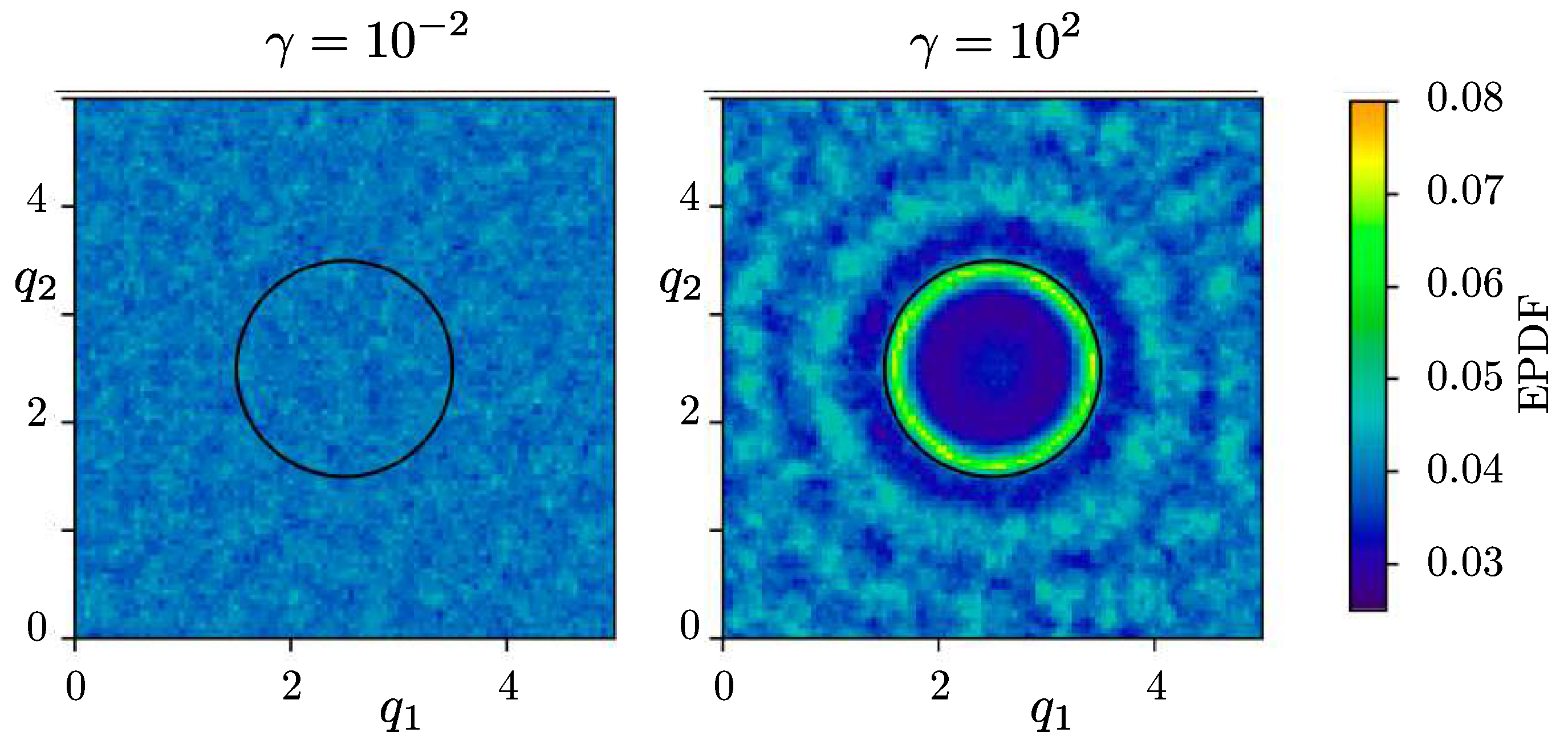
Due to the relatively small size of the heat source area the number of particles in this area is small in comparison to the number of particles outside of the heat source area and hence the shape of the radial density is mainly determined by the statistical properties of the particles outside the heat source area. The empirical particle densities shown in Figure 2 provide further insight into how the value of the friction coefficient affects the properties of . For a small friction coefficient, i.e., the particle density is very close to uniform on . If the heat bath temperature was constant in one would expect a uniform density as the potential function U is solely composed of pair potentials and thus translation-invariant in the coordinates of the particle density. More precisely, let and denote the first and second coordinate value of the i-th particle, then
for all . Therefore, the observed uniform particle density for is consistent with the observation that the position dependency of the effective temperature vanishes for this friction value. While for the considered trajectory length/sample size the plot of the invariant for a friction coefficient is very noisy, it still strongly suggests that the translation invariance of the particle density, i.e., the uniformity of the particle density, is broken in this regime. Within the interior of the heat source region particles are distributed approximately uniformly whereas close to the boundary of the heat source region the particle density is increased. Outside the heat source region the particle density is concentrated around positions close to energy minima of the potential energy function U.
5.2. System with Non-Conservative Force
We next consider an instance of a non-equilibrium system with a non-conservative force of a form as outlined in Section 3.2. More specifically, we let with and let the force be of the form (31), i.e.,
with
and
We furthermore assume that the system is driven by a standard Langevin diffusion, i.e.,
and
where we choose , and . This means, that without the non-conservative force part, i.e., in the case , the system considered resembles to a particle moving in a 4-well potential driven by a standard Langevin equation at equilibrium at unit temperature. The non-conservative force part , corresponds to a stirring force, which pushes the system radially and in clockwise direction around the origin. The effect of the stirring force can be seen in Figure 3. In the absence of the stirring force (see Figure 3A) the invariant distribution is exactly the canonical distribution, i.e.,
The modes of the marginal density in are exactly positioned at the energy minima of U at . Estimates of the mean momentum vectorfield
vanish at each point in the configurational phase space. In the presence of the stirring force (see Figure 3B), the invariant density is rotated slightly and smeared out over the energy barriers. The mean momentum resembles a vector field spiralling clockwise around the origin.
5.3. Stochastic Cucker-Smale Model
In this section we present simulation results for a modified stochastic Cucker-Smale model as described in Section 3.5.2. In particular, we demonstrate that the peculiar and consensus temperature as well as the consensus diffusion rate can be controlled independently and match in simulation with the analytically derived values, if the friction tensor and the diffusion tensor are suitably parametrized. Apart from these macroscopic quantities, we also demonstrate the effect of different parameter values of on other macroscopic quantities which in general do not possess a closed form, such as the radial density of particles and peculiar velocity autocorrelation function. Several animations of the particle motion, which effect of parameter choices, may be viewed at the following web location: https://github.com/MatthiasSachs/StochasticCuckerSmale.git.
5.3.1. Model Parametrization
If not stated otherwise the results presented in this section were obtained from a system of 64 particles in a periodic simulation box of edge length 5 and dimension 2, i.e., with and . We assume the particle pair-potentials in the definition of U to be identical Morse potentials, i.e., for
with . Following [4] we choose the functions in the definition of in (36) to be of the form
with , and .
5.3.2. Independent Control of Peculiar and Consensus Temperature
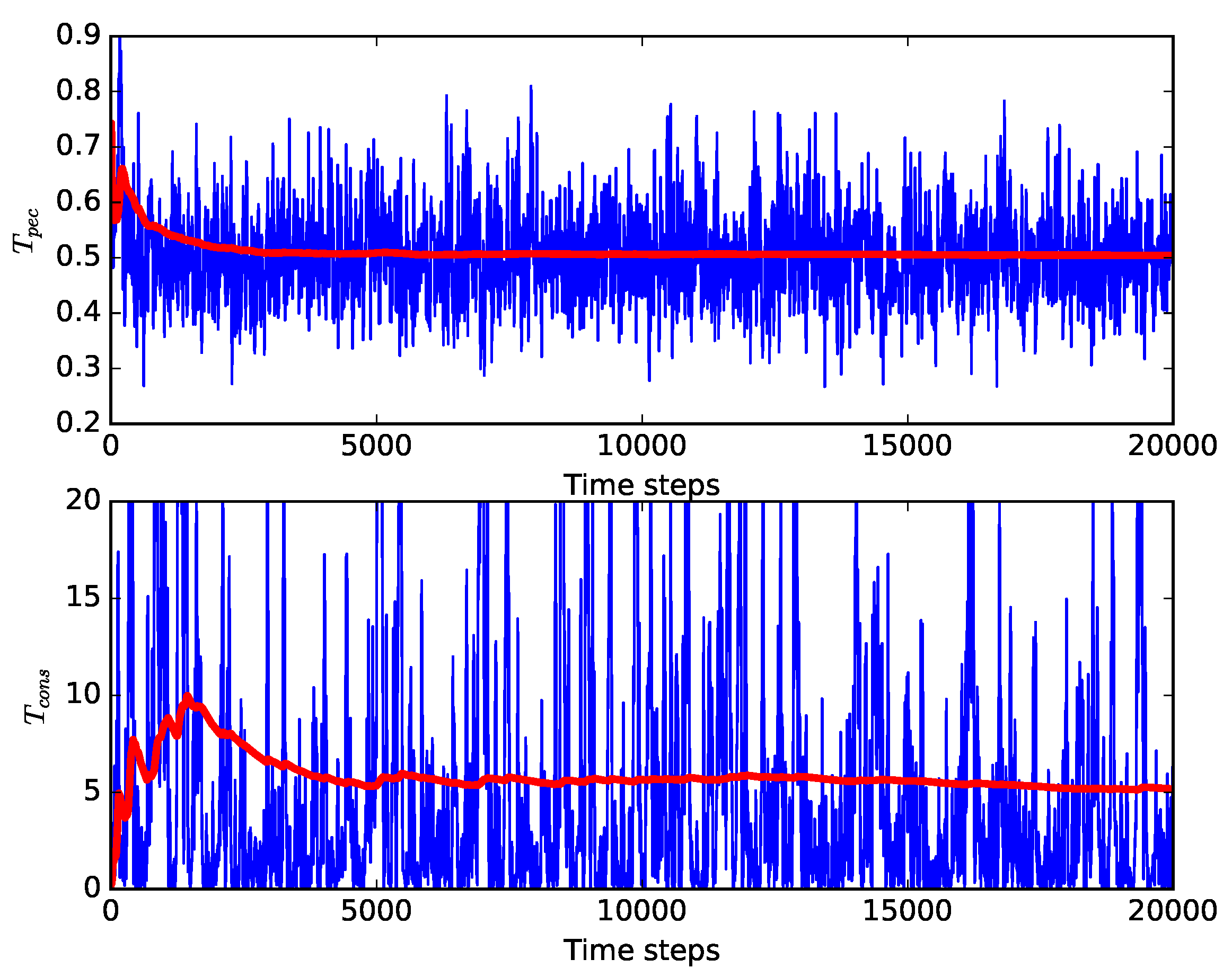
We first demonstrate that as stated in Proposition 1, we can indeed control the peculiar and the consensus temperature independently, such that these quantities coincide with the values of the model parameters and , respectively, i.e., we show that the identities (53) and (54) are reproduced in simulations. For this purpose we compute an estimate of the peculiar temperature at time step as
and an estimate of the consensus temperature at time step as
In Figure 4 we show the results for a system with and . We see that the cumulative average of the respective estimates converges, after a short equilibration period, to the target values.
5.3.3. Properties of the Flock
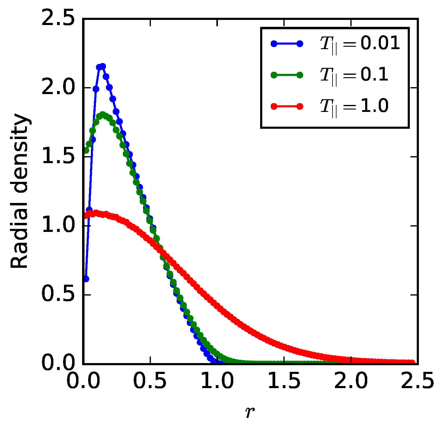
We first demonstrate the effect of the parameterization of the peculiar dynamics (the values of the peculiar friction and the peculiar temperature ) on the flock size, flock formation, and inter-flock diffusion. While we vary the values of the peculiar temperature parameter and peculiar friction parameter in order to demonstrate the effect of these parameters on the above quantities, we leave the parameter values of the consensus dynamics unchanged in all simulations as and . In the first series of simulations we vary the value of , while fixing the value of the peculiar friction parameter to . Figure 5 shows the radial density for different values of . As one would expect, the probability mass is concentrated around the mean rest-length of the Morse-potential for low values of and the distribution spreads out for higher values of . If we measure flock size in terms of the mean distance between particles in the flock, this implies that the flock size grows for increased temperature.
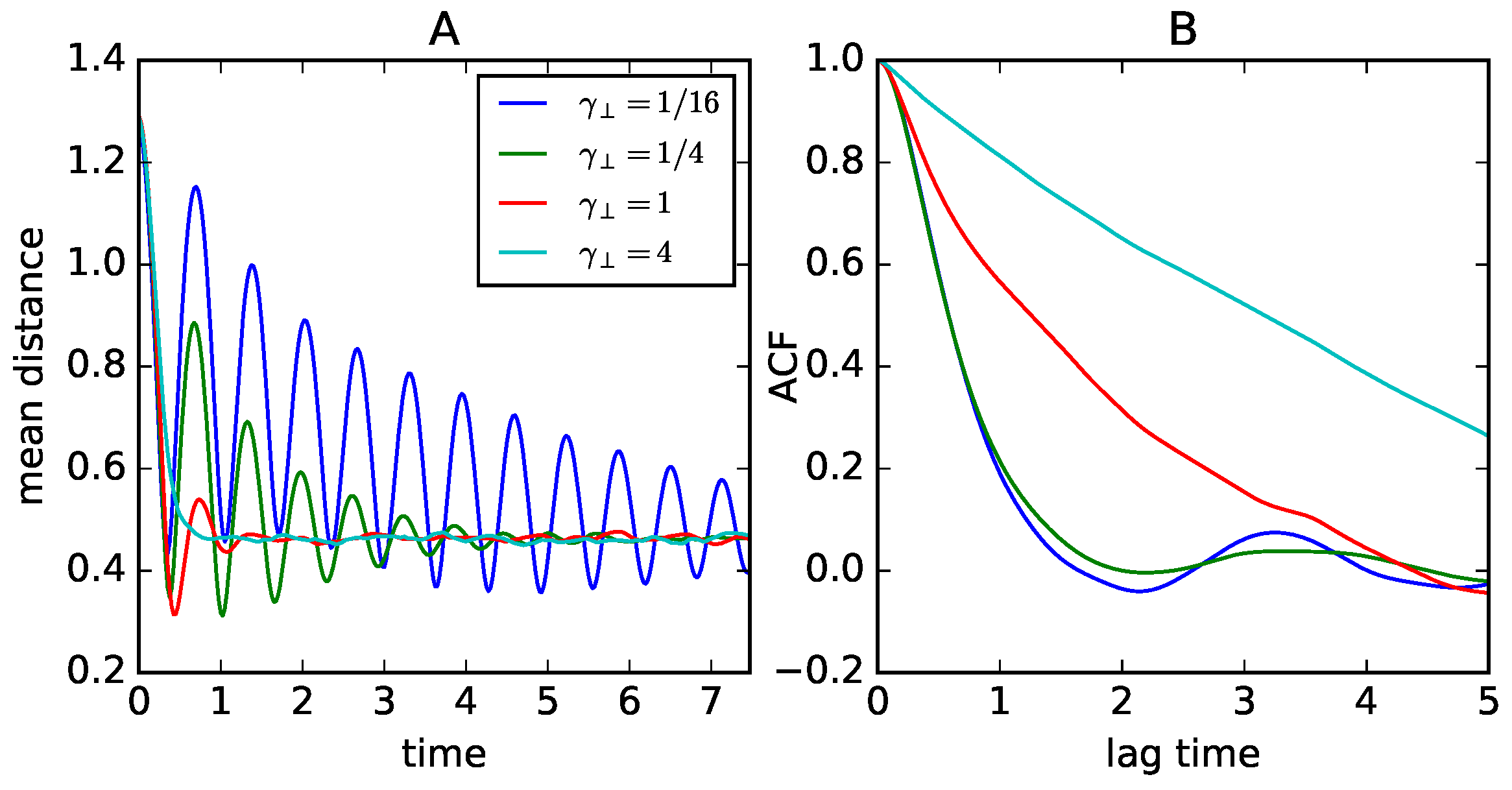
We next explore the effects of the peculiar friction parameter . We study the effect of the value of on the flock formation using the mean distance between particles,
as a measure of the progression of the flock formation. We initialize the particle position out of equilibrium on a equidistant square grid covering a square with side length . Figure 6A shows the time evolution of observed mean distance in simulations using different values of . We find that for small value of flock formation comes with strong oscillation in the flock size (measured in terms of the mean particle distance), which only slowly decays. With increased values of these oscillations are more strongly damped so that the flock size quickly approaches its equilibrium value.
We next explore the effect of the value of the model parameter on the mobility of particles within the flock. In order to measure the strength of diffusion within the flock we consider the mean distance of the particle i to the center of mass, i.e.,
The autocorrelation of this observable can be used as a measure of mobility within the flock. Figure 6B, shows the autocorrelation function for calculated from a trajectory in equilibrium, i.e., after the initial transitional flock-formation phase described in the previous paragraph. We can see that the decay of the autocorrelation function becomes slower for increasing values of , which indicates that for an increased value of the mobility of particles within the flock is reduced.
5.3.4. Collective Motion
We next explore the effects of the values of and on the collective motion of the flock, i.e., the diffusive behaviour of the center of mass. Since the motion of the center of mass is described by the consensus dynamics, which is driven by an Ornstein-Uhlenbeck process, we find the diffusion constant D of the center of mass (viewed as a free particle in space) to be
Table 1 shows the estimated diffusion coefficients for various values of and . We find a good match between theoretically predicted values and observed values.
6. Conclusions
In this article we have provided a general treatment of the convergence of Langevin dynamics to a stationary state, including for systems with configuration-dependent friction and noise, as well as nonconservative forces. We have demonstrated the concepts in applications to systems with temperature gradients and stochastic models of active particle systems. Our approach does not assume the usual fluctuation-dissipation rule, so it can be applied to a wide range of nonequilibrium molecular and particle systems where the form of the stationary distribution is a priori unknown. Future work might look at the use of configuration-dependent memory kernels (within a generalized Langevin equation setting) and proofs of ergodicity for degenerate thermostats, for example the pairwise adaptive thermostats [40], which provide an alternative method for controlling observables.
Acknowledgments
The research of all three authors was supported by the ERC project RULE (grant number 320823). The collaboration was initiated during a residency of the first two authors at the Institut Henri Poincaré and its program on “Stochastic dynamics out of equilibrium.” The work of M. Sachs was further supported by the Statistical and Applied Mathematical Sciences Institute (North Carolina).
Author Contributions
The article was conceived in joint discussions of all three authors during May of 2017. All three authors contributed to the writing. The numerical experiments were proposed and discussed by all three authors but were performed by M.S.
Conflicts of Interest
The authors declare no conflict of interest.
References
- Lancon, P.; Batrouni, G.; Lobry, L.; Ostrowsky, N. Drift without flux: Brownian walker with a space-dependent diffusion coefficient. Europhys. Lett. 2001, 54, 28–34. [Google Scholar] [CrossRef]
- Regev, S.; Grønbech-Jensen, N.; Farago, O. Isothermal Langevin dynamics in systems with power-law spatially dependent friction. Phys. Rev. E 2016, 94, 012116. [Google Scholar] [CrossRef] [PubMed]
- Becton, M.; Wang, X. Thermal gradients on graphene to drive nanoflake motion. J. Chem. Theory Comput. 2014, 10, 722–730. [Google Scholar] [CrossRef] [PubMed]
- Cucker, F.; Mordecki, E. Flocking in noisy environments. J. Math. Pures Appl. 2008, 89, 278–296. [Google Scholar] [CrossRef]
- Ha, S.Y.; Lee, K.; Levy, D. Emergence of time-asymptotic flocking in a stochastic Cucker-Smale system. Commun. Math. Sci. 2009, 7, 453–469. [Google Scholar] [CrossRef]
- Gachelin, J.; Rousselet, A.; Lindner, A.; Clement, E. Collective motion in an active suspension of Escherichia coli bacteria. New J. Phys. 2014, 16, 025003. [Google Scholar] [CrossRef]
- Best, R.; Hummer, G. Coordinate-dependent diffusion in protein folding. Proc. Natl. Acad. Sci. USA 2010, 107, 1088–1093. [Google Scholar] [CrossRef] [PubMed]
- Chen, C.; Liu, S.; Shi, X.Q.; Chaté, H.; Wu, Y. Weak synchronization and large-scale collective oscillation in dense bacterial suspensions. Nature 2017, 542, 210–214. [Google Scholar] [CrossRef] [PubMed]
- Hoogerbrugge, P.; Koelman, J. Simulating microscopic hydrodynamic phenomena with dissipative particle dynamics. Europhys. Lett. 1992, 19, 155–160. [Google Scholar] [CrossRef]
- Español, P. Dissipative particle dynamics. In Handbook of Materials Modeling; Springer: Berlin, Germany, 2005; pp. 2503–2512. [Google Scholar]
- Shardlow, T.; Yan, Y. Geometric ergodicity for dissipative particle dynamics. Stoch. Dyn. 2006, 6, 123–154. [Google Scholar] [CrossRef]
- Ahn, S.; Ha, S.Y. Stochastic flocking dynamics of the Cucker-Smale model with multiplicative white noises. J. Math. Phys. 2010, 51, 103301. [Google Scholar] [CrossRef]
- Ton, T.; Linh, N.; Yagi, A. Flocking and non-flocking behavior in a stochastic Cucker-Smale System. Anal. Appl. 2014, 12, 63–73. [Google Scholar] [CrossRef]
- Erban, R.; Haskovec, J.; Sun, Y. A Cucker-Smale model with noise and delay. SIAM J. Appl. Math. 2016, 76, 535–1557. [Google Scholar] [CrossRef]
- Leimkuhler, B.; Matthews, C.; Stoltz, G. The computation of averages from equilibrium and nonequilibrium Langevin molecular dynamics. IMA J. Numer. Anal. 2016, 36, 13–79. [Google Scholar] [CrossRef]
- Leimkuhler, B.; Matthews, C. Rational construction of numerical methods for stochastic molecular dynamics. Appl. Math. Res. Exp. 2013, 2013, 34–56. [Google Scholar]
- Tuckerman, M.; Berne, B.J.; Martyna, G.J. Reversible multiple time scale molecular dynamics. J. Chem. Phys. 1992, 97, 1990–2001. [Google Scholar] [CrossRef]
- Hummer, G. Position-dependent diffusion coefficients and free energies from Bayesian analysis of equilibrium and replica molecular dynamics simulations. New J. Phys. 2005, 7, 34. [Google Scholar] [CrossRef]
- Burada, P.; Schmid, G.; Reguera, D.; Rubi, J.; Hänggi, P. Biased diffusion in confined media: Test of the Fick-Jacobs approximation and validity criteria. Phys. Rev. E 2007, 75, 051111. [Google Scholar] [CrossRef] [PubMed]
- Berezhkovskii, A.; Szabo, A. Time scale separation leads to position-dependent diffusion along a slow coordinate. J. Chem. Phys. 2011, 135, 074108. [Google Scholar] [CrossRef] [PubMed]
- Wilmer, O.R.; Pedro, C.; Lopez, F. Direct evaluation of the position dependent diffusion coefficient and persistence time from the equilibrium density profile in anisotropic fluids. J. Chem. Phys. 2013, 139, 074103. [Google Scholar]
- Lelièvre, T.; Stoltz, G. Partial differential equations and stochastic methods in molecular dynamics. Acta Numer. 2016, 25, 681–880. [Google Scholar] [CrossRef]
- Bellet, L.R. Ergodic properties of Markov processes. In Open Quantum Systems II; Springer: Berlin, Germany, 2006; pp. 1–39. [Google Scholar]
- Gardiner, C. Handbook of stochastic methods for physics, chemistry and the natural sciences. Appl. Opt. 1986, 25, 3145. [Google Scholar] [CrossRef]
- Guionnet, A.; Zegarlinksi, B. Lectures on logarithmic Sobolev inequalities. In Séminaire de Probabilités XXXVI; Springer: Berlin, Germany, 2003; pp. 1–134. [Google Scholar]
- Hörmander, L. The Analysis of Linear Partial Differential Operators. III, Volume 274 of Grundlehren der Mathematischen Wissenschaften [Fundamental Principles of Mathematical Sciences]; Springer: Berlin, Germany, 1985. [Google Scholar]
- Kliemann, W. Recurrence and invariant measures for degenerate diffusions. Ann. Probab. 1987, 15, 690–707. [Google Scholar] [CrossRef]
- Bhattacharya, R.N. On the functional central limit theorem and the law of the iterated logarithm for Markov processes. Zeitschrift Für Wahrscheinlichkeitstheorie Und Verwandte Gebiete 1982, 60, 185–201. [Google Scholar] [CrossRef]
- Villani, C. Hypocoercivity; Number 949-951; American Mathematical Society: Providence, RI, USA, 2009. [Google Scholar]
- Dolbeault, J.; Mouhot, C.; Schmeiser, C. Hypocoercivity for linear kinetic equations conserving mass. Trans. Am. Math. Soc. 2015, 367, 3807–3828. [Google Scholar] [CrossRef]
- Harris, T.E. The existence of stationary measures for certain Markov processes. In Proceedings of the Third Berkeley Symposium on Mathematical Statistics and Probability, Volume 2: Contributions to Probability Theory; University of California Press: Oakland, CA, USA, 1956; pp. 113–124. [Google Scholar]
- Meyn, S.P.; Tweedie, R.L. Stability of Markovian processes I: Criteria for discrete-time chains. Adv. Appl. Probab. 1992, 24, 542–574. [Google Scholar] [CrossRef]
- Hairer, M.; Mattingly, J.C. Yet another look at Harris’ ergodic theorem for Markov chains. In Seminar on Stochastic Analysis, Random Fields and Applications VI; Springer: Berlin, Germany, 2011; Volume 63, pp. 109–117. [Google Scholar]
- Meyn, S.P.; Tweedie, R.L. Stability of Markovian processes III: Foster–Lyapunov criteria for continuous-time processes. Adv. Appl. Probab. 1993, 25, 518–548. [Google Scholar]
- Mattingly, J.C.; Stuart, A.M.; Higham, D.J. Ergodicity for SDEs and approximations: Locally Lipschitz vector fields and degenerate noise. Stoch. Process. Their Appl. 2002, 101, 185–232. [Google Scholar] [CrossRef]
- Meyn, S.P.; Tweedie, R.L. Markov Chains and Stochastic Stability; Springer Science & Business Media: Berlin, Germany, 2012. [Google Scholar]
- Zhang, F. The Schur Complement and Its Applications; Springer Science & Business Media: Berlin, Germany, 2006; Volume 4. [Google Scholar]
- Cucker, F.; Smale, S. Emergent behavior in flocks. IEEE Trans. Autom. Control 2007, 52, 852–862. [Google Scholar] [CrossRef]
- Groot, R.D.; Warren, P.B. Dissipative particle dynamics: Bridging the gap between atomistic and mesoscopic simulation. J. Chem. Phys. 1997, 107, 4423–4435. [Google Scholar] [CrossRef]
- Leimkuhler, B.; Shang, X. Pairwise adaptive thermostats for improved accuracy and stability in dissipative particle dynamics. J. Comput. Phys. 2016, 324, 174–193. [Google Scholar] [CrossRef]
Figure 1.
(A) Radial density function for the particle system described in Section 5.1 for different values of the friction coefficient ; (B) Distance r from heat source center vs. effective temperature estimated according to (65). The black curve corresponds to the heat bath temperature , with as defined in (64).
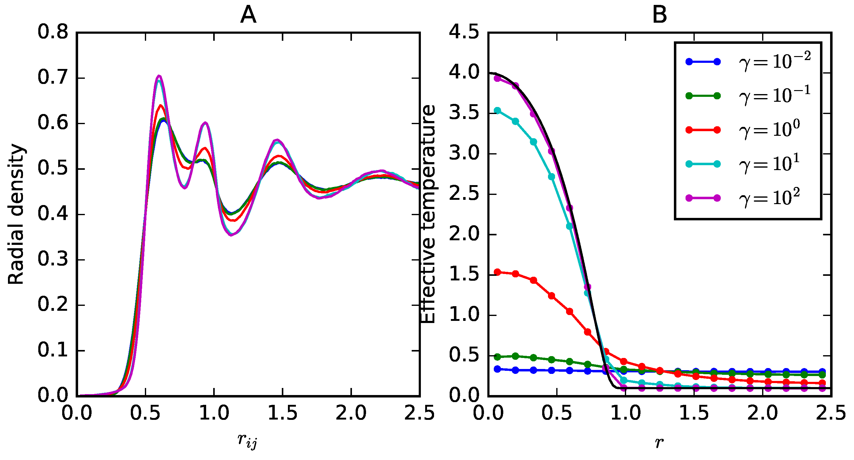
Figure 2.
Empirical particle density calculated as a cumulative average over the simulation time, for two values of . The area inside the black circle corresponds to the heat source area.
Figure 2.
Empirical particle density calculated as a cumulative average over the simulation time, for two values of . The area inside the black circle corresponds to the heat source area.

Figure 3.
Marginal of of the invariant density of the system described in Section 5.2 in the absence () of the non-conservative force (A), and in the presence () of the non-conservative force (B). The black arrows correspond to estimates of the mean momentum vector field (66) in the invariant density at the respective points in configurational space.
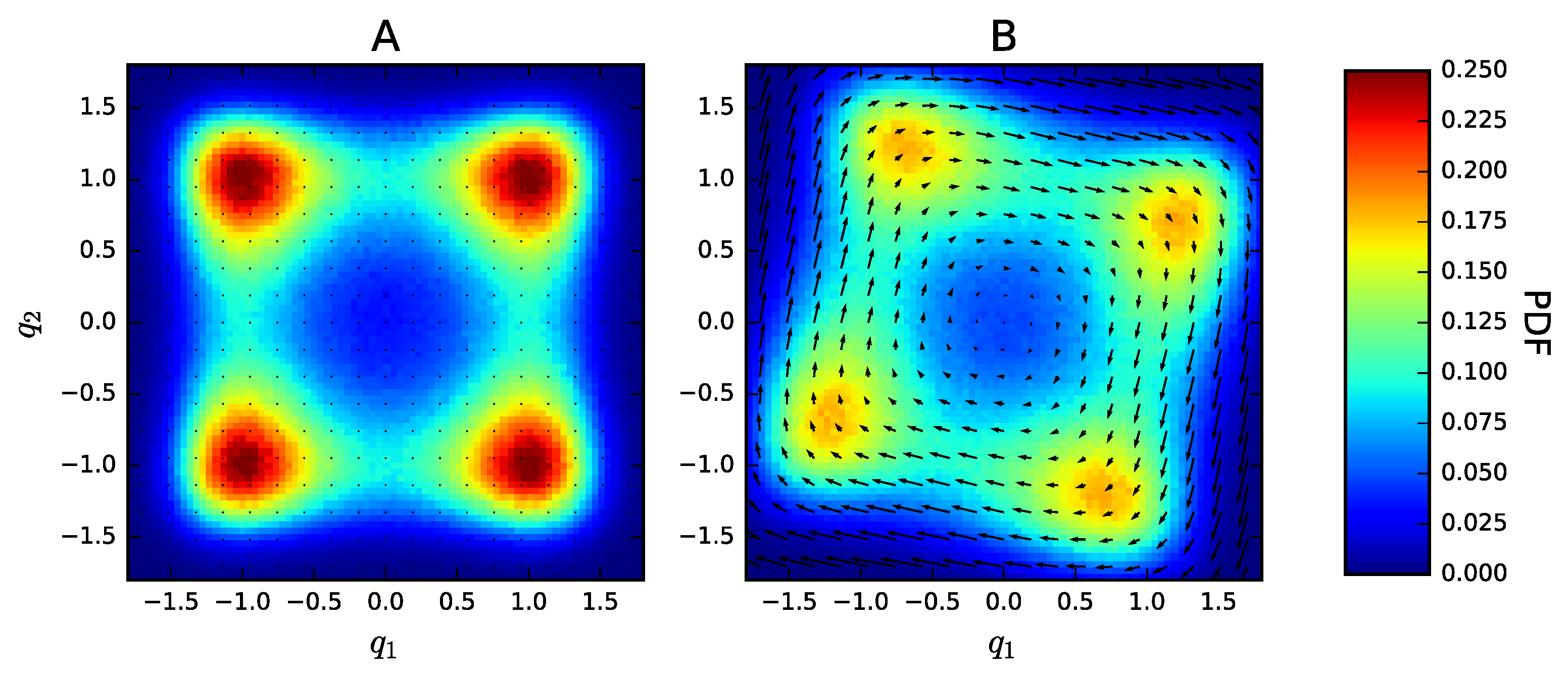
Figure 4.
Time vs. observed peculiar temperature (upper figure) and consensus temperature (lower figure). The blue trajectory shows the estimates and at timestep k for the peculiar and the consensus temperature, respectively. The respective cumulative averages are shown in red.
Figure 4.
Time vs. observed peculiar temperature (upper figure) and consensus temperature (lower figure). The blue trajectory shows the estimates and at timestep k for the peculiar and the consensus temperature, respectively. The respective cumulative averages are shown in red.

Figure 5.
Radial density function for varying values of the peculiar temperature parameter .

Figure 6.
Flock formation and inter-flock diffusion for different values of the peculiar friction parameter . (A) Time vs. mean distance ; (B) Lag time vs. time-autocorrelation of the mean-centre distance . The plotted curve is computed as an average over all particles indices .
Figure 6.
Flock formation and inter-flock diffusion for different values of the peculiar friction parameter . (A) Time vs. mean distance ; (B) Lag time vs. time-autocorrelation of the mean-centre distance . The plotted curve is computed as an average over all particles indices .


Table 1.
Estimates of for various values of and . denotes the number of particles and D the diffusion coefficient of the diffusive motion of the center of mass. Values in parentheses show the exact values.
Table 1.
Estimates of for various values of and . denotes the number of particles and D the diffusion coefficient of the diffusive motion of the center of mass. Values in parentheses show the exact values.
| 1 | 10 | 100 | |
|---|---|---|---|
| 1 | 0.987, (1) | 9.775, (10) | 101.8, (100) |
| 3 | 3.059, (3) | 29.445, (30) | 308.1, (300) |
| 9 | 8.476, (9) | 91.994, (90) | 861.4, (900) |
© 2017 by the authors. Licensee MDPI, Basel, Switzerland. This article is an open access article distributed under the terms and conditions of the Creative Commons Attribution (CC BY) license (http://creativecommons.org/licenses/by/4.0/).
Share and Cite
MDPI and ACS Style
Sachs, M.; Leimkuhler, B.; Danos, V. Langevin Dynamics with Variable Coefficients and Nonconservative Forces: From Stationary States to Numerical Methods. Entropy 2017, 19, 647. https://doi.org/10.3390/e19120647
AMA Style
Sachs M, Leimkuhler B, Danos V. Langevin Dynamics with Variable Coefficients and Nonconservative Forces: From Stationary States to Numerical Methods. Entropy. 2017; 19(12):647. https://doi.org/10.3390/e19120647
Chicago/Turabian StyleSachs, Matthias, Benedict Leimkuhler, and Vincent Danos. 2017. "Langevin Dynamics with Variable Coefficients and Nonconservative Forces: From Stationary States to Numerical Methods" Entropy 19, no. 12: 647. https://doi.org/10.3390/e19120647
Note that from the first issue of 2016, this journal uses article numbers instead of page numbers. See further details here.