K-Dependence Bayesian Classifier Ensemble


Key Laboratory of Symbolic Computation and Knowledge Engineering of Ministry of Education, Jilin University, Changchun 130012, China
*
Author to whom correspondence should be addressed.
Entropy 2017, 19(12), 651; https://doi.org/10.3390/e19120651
Submission received: 6 September 2017
/
Revised: 23 November 2017
/
Accepted: 27 November 2017
/
Published: 30 November 2017
(This article belongs to the Special Issue Symbolic Entropy Analysis and Its Applications)
Abstract
:To maximize the benefit that can be derived from the information implicit in big data, ensemble methods generate multiple models with sufficient diversity through randomization or perturbation. A k-dependence Bayesian classifier (KDB) is a highly scalable learning algorithm with excellent time and space complexity, along with high expressivity. This paper introduces a new ensemble approach of KDBs, a k-dependence forest (KDF), which induces a specific attribute order and conditional dependencies between attributes for each subclassifier. We demonstrate that these subclassifiers are diverse and complementary. Our extensive experimental evaluation on 40 datasets reveals that this ensemble method achieves better classification performance than state-of-the-art out-of-core ensemble learners such as the AODE (averaged one-dependence estimator) and averaged tree-augmented naive Bayes (ATAN).
1. Introduction
Classification is a basic task in data analysis and pattern recognition that requires the learning of a classifier, which assigns labels or categories to instances described by a set of predictive variables or attributes. The induction of classifiers from datasets of preclassified instances is a central problem in machine learning. Given class label C and predictive attributes ( capital letters, such as and Z, denote attribute names, and lowercase letters, such as x, y and z, denote the specific values taken by those attributes. Sets of attributes are denoted by boldface capital letters, such as , and , and assignments of values to the attributes in these sets are denoted by boldface lowercase letters, such as and ), discriminative learning [1,2,3,4] directly models the conditional probability . Unfortunately, cannot be decomposed into a separate term for each attribute, and there is no known closed-form solution for the optimal parameter estimates. Generative learning [5,6,7,8] approximates the joint probability with different factorizations according to Bayesian network classifiers, which are powerful tools for knowledge representation and inference under conditions of uncertainty. Naive Bayes (NB) [9], which is the simplest kind of Bayesian network classifier that assumes the attributes are independent given the class label, are surprisingly effective. After the discovery of NB, many state-of-the-art algorithms, for example, tree-augmented naive Bayes (TAN) [10] and a k-dependence Bayesian classifier (KDB) [11], are proposed to relax the independence assumption by allowing conditional dependence between attributes and , which is measured by conditional mutual information . In order to improve predictive accuracy relative to a single model, ensemble methods [12,13], for example, averaged one-dependence estimator (AODE) [14] and averaged tree-augmented naive Bayes (ATAN) [15] methods, generate multiple global models from a single learning algorithm through randomization (or perturbation).
An ideal Bayesian network classifier should provide the maximum value of mutual information for classification; that is, should represent strong mutual dependence between C and . However,
The strong conditional dependence between attributes and may not help to improve classification performance. As shown in Figure 1, the proportional distribution of differs greatly to that of .
The KDB is a form of a restricted Bayesian network classifier with numerous desirable properties in the context of learning from large quantities of data. It achieves a good trade-off between classification performance and structure complexity with a single parameter, k. KDB uses mutual information to predetermine the order of predictive attributes and conditional mutual information to measure the conditional dependence between predictive attributes.
In this paper, we extend the KDB. The contributions of this paper are as follows:
- We propose a new sorting method to predetermine the order of predictive attributes. This sorting method considers not only the dependencies between predictive attributes and the class variable, but also the dependencies between predictive attributes.
- We extend the KDB from one single k-dependence tree to a k-dependence forest (KDF). A KDF reflects more dependencies between predictive attributes than the KDB. We show that our algorithm achieves comparable or lower error on University of California at Irvine (UCI) datasets than a range of popular classification learning algorithms.
The rest of this paper is organized as follows. Section 2 introduces some state-of-the-art Bayesian network classifiers. Section 3 explains the basic idea of the KDF and introduces the learning procedure in detail. Section 4 compares experimental results on datasets from the UCI Machine Learning Repository. Section 5 draws conclusion.
2. Bayesian Network Classifiers
A Bayesian network [16], , is a directed acyclic graph with a conditional probability distribution for each node, collectively represented by , which quantifies how much a node depends on its parents. Nodes and arcs in G represent random variables and the probability dependence between variables, respectively. The full Bayesian network classifier [17] fully reflects the dependencies between predictive attributes and can be regarded as the optimal Bayesian network classifier. The corresponding joint probability is
From Equation (1), we can see that the true complexity in such an unrestricted model (i.e., no independencies) comes from the large number of attribute dependence arcs that are present in the model. As the number of attributes and arcs increase, the computational complexity of the joint probability grows exponentially until it becomes an NP-hard problem [18]. In order to address this issue, researchers have proposed some state-of-the-art classifiers to simplify the network structure [9,19,20,21]. The functional domain of one single classifier may be limited as a result of ignoring the dependencies between some attributes. Classifiers that use the forest or ensemble method are commonly applied to fill the gap [12,14,15]. In the following subsection, we first introduce NB and its corresponding ensemble classifier, that is, AODE. Then, we introduce TAN and its corresponding ensemble classifier, that is, ATAN. Lastly, we introduce the KDB in detail.
2.1. NB and AODE
NB, which is the simplest Bayesian network classifier, supposes that all the predictive attributes are independent of each other given class variable C, transforming Equation (1) into
NB has exhibited a high level of predictive competence with other learning algorithms, such as decision trees [22]. However, in the real world, attributes in many learning tasks are correlated to each other, so the conditional independence assumption rarely holds and it may degrade the classification performance. How to relax the conditional independence assumption and simultaneously retain NBs’ efficiency have attracted much attention, and many approaches have been proposed already [11,14,19].
AODE is an ensemble augmentation of NB that utilizes a restricted class of one-dependence estimators (ODEs) and aggregates the predictions of all qualified estimators within this class. A single attribute , called a superparent, is selected as the parent of all the other attributes in each ODE. For each ODE, AODE utilizes an assumption that the attributes are independent given the class variable and any predictive attribute , estimating Equation (1) by
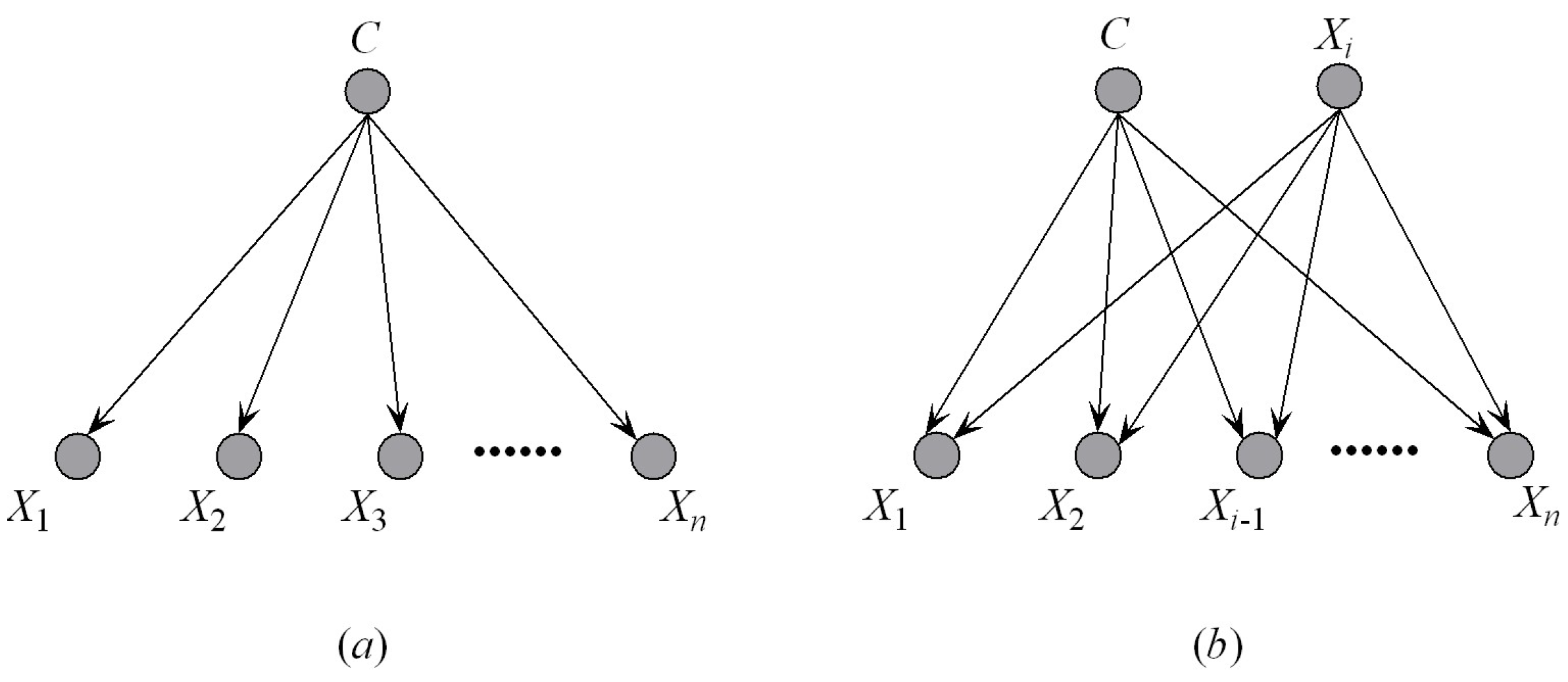
AODE achieves lower classification error than NB, because it involves a weaker attribute independence assumption and the ensemble mechanism. Figure 2 shows graphically the structural differences between NB and AODE.
2.2. TAN and ATAN
TAN is a structural augmentation of NB in which every attribute has the class and at most one other attribute as parents. The structure is determined by using an extension of the Chow–Liu tree [23], which utilizes conditional mutual information to find a maximum spanning tree. By learning from the maximum weighted spanning tree (MWST), TAN can represent all significant one-dependence relationships and is commonly regarded as the optimal one-dependence classifier [24]. Rather than obtaining a spanning tree, Ruz and Pham [25] suggest that Kruskal’s algorithm be stopped whenever a Bayesian criterion controlling the likelihood of the data and the complexity of the TAN structure holds.
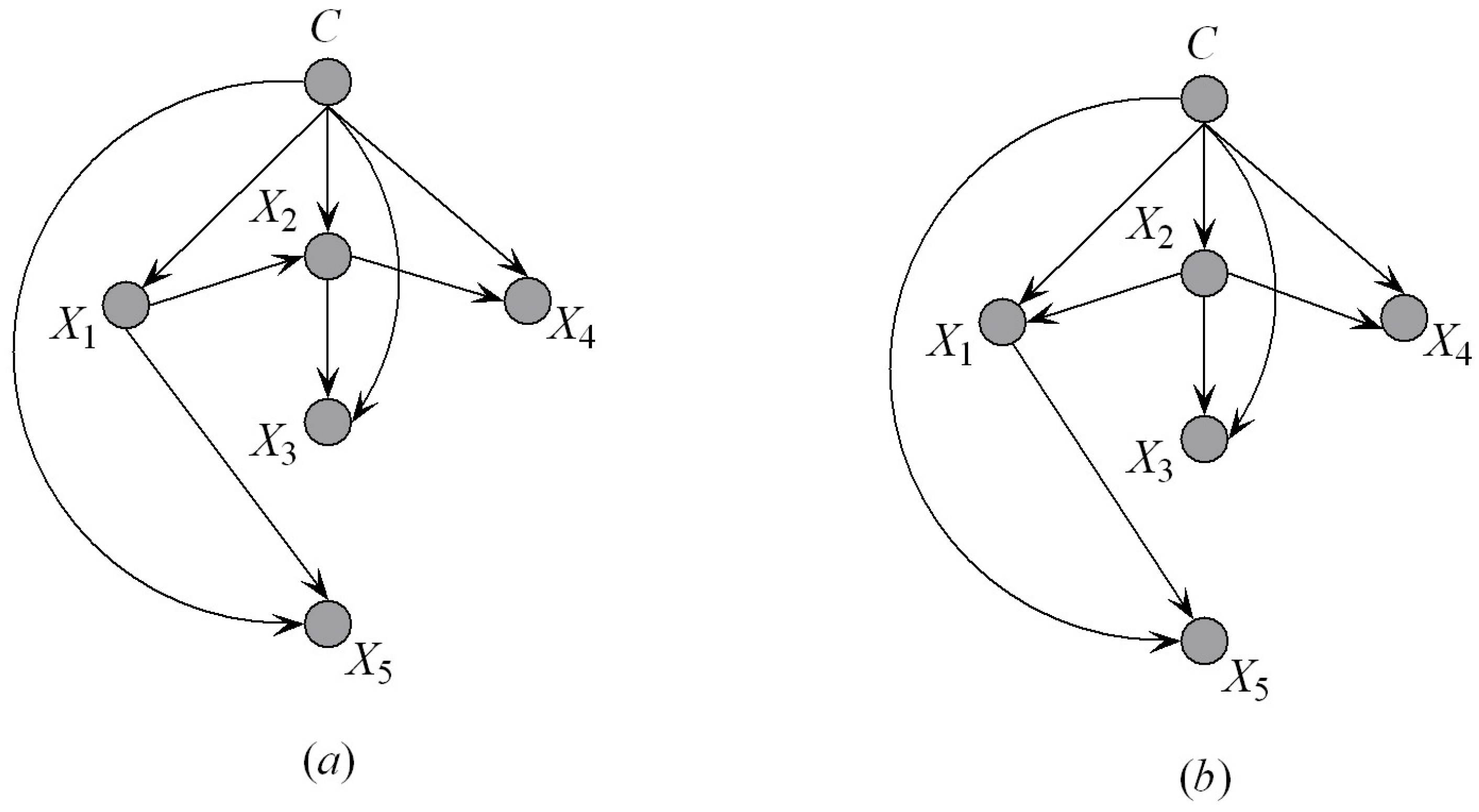
ATAN is an ensemble augmentation of TAN. It takes not a random node, but each predictive variable as a root node and then builds the corresponding MWST conditioned to that selection. Finally, the posterior probabilities of ATAN are given by the average of the n TAN classifier posterior probabilities. Figure 3 shows graphically the structural differences between TAN and ATAN.
2.3. KDB
The KDB allows each attribute to have a maximum of k parents, except the class variable. The attribute order is predetermined by comparing mutual information between the predictive attribute and class variable, starting with the highest. Once enters the model, its parents are selected by choosing the k variables in the model with the highest values of the conditional mutual information . We note that the first k variables added to the model will have fewer than k parents. We suppose that the attribute order is ; then will have parents when , and the remaining variables have exactly k parents. Then Equation (1) turns out to be
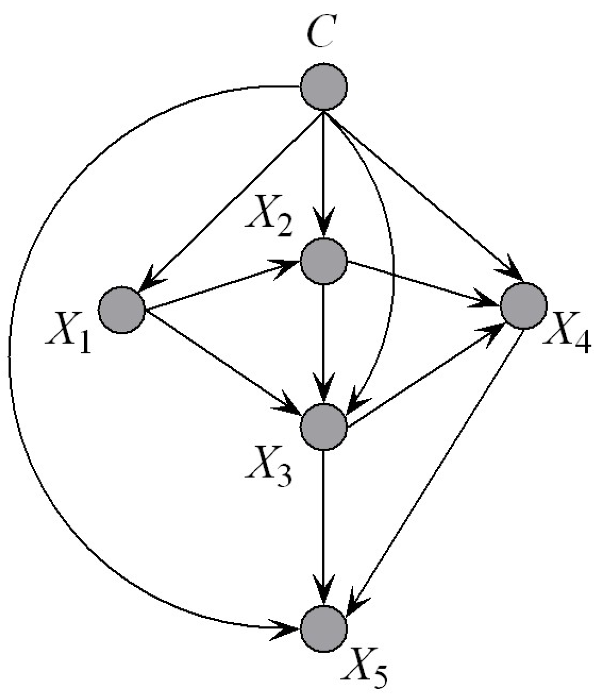
where are the parent attributes of and . Figure 4 shows graphically an example of a KDB.
3. The k-Dependence Forest Algorithm
The KDB is supplied with both a database of preclassified instances, a DB, and the k value for the maximum allowable degree of attribute dependence. The structure learning procedure of a KDB can be partitioned into two parts: attribute sorting and dependence analysis. During the sorting procedure, the KDB uses mutual information to predetermine the order of predictive attributes. The KDB ensures that the predictive attributes that are most dependent on the class variable should be considered first and added to the structure. However, mutual information can only measure the dependencies between predictive attributes and the class variable, while it ignores the dependencies between predictive attributes. The sorting process of the KDB only embodies the dependency between each single attribute and class variable, which may result in a suboptimal order. The proposed algorithm, the KDF, uses a new sorting method to address this issue.
According to the chain rule of information theory, mutual information can be expanded as follows:
In the ideal case, in classification, we would like to obtain the maximum value of . From Equation (5), we can find that the computational complexity of grows exponentially as the number of attributes increases. The space to store the conditional probability distribution grows exponentially. How to approximate the probability estimation is challenging. In order to address this issue, we replace with the following:
Equation (6) considers both the mutual dependence and the conditional dependence for classification. On the basis of this, we propose a new approach to predetermine the sequence of predictive attributes by comparing the value of . From Equation (6), we can find that the first attribute of a sequence does not reflect the conditional dependence. Thus we use each attribute as the root node in turn. The next attribute, which will be added to the sequence, is the attribute that is most informative about C conditioned on the first attribute (which is measured by ). Subsequent attributes are chosen to be the most informative about C conditioned on previously chosen attributes (which is measured by ). Because of the n different root nodes, we can obtain n sequences {S, ⋯, S}. On the basis of the n sequences, n subclassifiers can be generated. The sorting algorithm (Algorithm 1) is depicted below.
| Algorithm 1: KDF: Sorting |
| Input: Preclassified dataset DB with n predictive attributes . Output: Sequences {S, ⋯, S}. For each sequence , :
|
In order to identify the graphical structure of the resulting classifier, the KDB adopts a greedy search strategy. The weight of conditional dependence between and its parent is measured by conditional mutual information . However, the dependency relationships between and other parents of are neglected, whether they are independent or strongly correlated. From Equation (1), we can see that, for the full Bayesian network classifier, the parent of is , the parent of is , the parent of is , and so forth. Then we can achieve an implicit chain rule, that is the parent of , is the parent of (or is the grandparent of ), is the parent of (or is the great grandparent of ), and so forth. Thus, as shown in Figure 5, there should exist hierarchical dependency relationships among the parents. If is one parent of attribute , we should follow the dotted line shown in Figure 5 to find the other parents. To make our idea clear, we first introduce the definition of an ancestor node.
Definition 1.
Suppose that is the parent of . The ancestor attributes of include ’s parents, grandparents, great grandparents, and so forth.
During the procedure of dependence analysis, first selects the attribute that corresponds to the largest value of as its parent. For the other parents, will select among its ancestor attributes. Figure 6a shows an example of the KDF subclassifier, for example, KDF. We suppose that . When is added to KDF, will be selected as the first parent of . The corresponding parent–child relationships are shown in Figure 6b, from which we can see that the ancestor attributes of are , that is, . Other parents of will be selected from by comparing . This strategy helps to reduce the search space of attribute dependencies. The detailed procedure of dependence analysis (Algorithm 2) is depicted below.
| Algorithm 2: KDF: Dependence Analysis |
| Input: Sequences {S, ⋯, S}. Output: Subclassifiers {KDF, ⋯, KDF}.
|
After training multiple learning subclassifiers, ensemble learning treats these as a “committee” of decision makers and combines individual predictions appropriately. The decision of the committee should have better overall accuracy, on average, than any individual committee member. There exist numerous methods for model combination, for example, the linear combiner, the product combiner and the voting combiner. For the subclassifier KDF, an estimate of the probability of class c given input is . The linear combiner is used for models that output real-valued numbers; thus it is applicable for the KDF. The ensemble probability estimate is
If the weights , , this is a simple uniform averaging of the probability estimates. The notation clearly allows for the possibility of a nonuniformly weighted average. If the classifiers have different accuracies on the data, a nonuniform combination could in theory give a lower error than a uniform combination. However, in practice, the difficulty is of estimating the parameters without overfitting and the relatively small gain that is available. Thus, in practice, we use the uniformly rather than nonuniformly weighted average.
The KDF collects the statistics to perform calculations of conditional mutual information of each pair of attributes given the class for structure learning. As an entry must be updated for every training instance and every combination of two attribute values for that instance, the time complexity of forming the three-dimensional probability table is , where m is the number of training instances, n is the number of attributes, c is the number of classes, and v is the maximum number of discrete values that any attribute may take. To calculate the conditional mutual information, the KDF must consider every pairwise combination of their respective values in conjunction with each class value . For each subclassifier KDF, attribute ordering and parent assignment are and , respectively. KDF requires n tables of dimensions, with . Because the KDF needs to average the results of n subclassifiers, the time complexity of classifying a single testing instance is time.
The parameter k is closely related to the classification performance of a high-dependence classifier. A higher value of k may result in higher variance and lower bias. Unfortunately there is no a priori means to preselect an appropriate value of k that can help to achieve the lowest error for a given training set, as this is a complex interplay between the data quantity and the complexity and strength of the interactions between the attributes proved by Martinez et al. [8]. From the discussion above, we can see that, for each KDF, the space complexity of the probability table increases exponentially as k increases; to achieve the trade-off between classification performance and efficiency, we restrict the structure complexity to be two-dependence, which is also adopted by Webb et al. [26].
4. Experiments and Results
In order to verify the efficiency and effectiveness of the proposed KDF algorithm, experiments were conducted on 40 benchmark datasets from the UCI Machine Learning Repository [27]. Table 1 summarizes the characteristics of each dataset, including the number of instances, attributes and classes. All the datasets were ordered by dataset scale. Missing values for qualitative attributes were replaced with modes, and those for quantitative attributes were replaced with means from the training data. For each original dataset, we discretized numeric attributes using minimum description length (MDL) discretization [28]. All experiments were conducted on a desktop computer with an Intel(R) Core(TM) i3-6100 CPU @ 3.70 GHz, 64 bits and 4096 MB of memory. All the experiments for the Bayesian algorithms used C++ software specifically designed to deal with classification methods. The running efficiency of the KDF was good. For example, for a Poker hand dataset, it took 281 s for the KDF to obtain classification results. The following algorithms were compared:
- NB, standard naive Bayes.
- TAN, tree-augmented naive Bayes.
- AODE, averaged one-dependence estimator.
- KDB, k-dependence Bayesian classifier.
- KDB, the KDB that only performs the sorting method proposed above.
- ATAN, averaged tree-augmented naive Bayes.
- RF100, random forest containing 100 trees.
- RFn, random forest containing n trees, where n is the number of predictive attributes.
- KDF, k-dependence forest.
Kohavi and Wolpert presented a bias-variance decomposition of the expected misclassification rate [29], which is a powerful tool from sampling theory statistics for analyzing supervised learning scenarios. Supposing c and are the true class label and that generated by a learning algorithm, respectively, the zero-one loss function is defined as
The bias term measures the squared difference between the average output of the target and the algorithm. This term is defined as follows:
where is the combination of any attribute value. The variance term is a real-valued non-negative quantity that equals zero for an algorithm that always makes the same guess regardless of the training set. The variance increases as the algorithm becomes more sensitive to changes in the training set. It is defined as follows:
Given the definite Bayesian network structure, can be calculated as follows:
The conditional probability in the bias term can be rewritten as
Given a dataset containing e test instances, the values of zero-one loss, bias and variance for this dataset can be achieved by averaging the result of zero-one loss, bias and variance for all test instances.
In order to clarify the performance of the KDF over datasets of a different scale, we propose a new scoring criterion, which is called goal difference (GD).
Definition 2.
Goal difference (GD) is a scoring criterion to compare the performance of two classifiers. Given two classifiers A and B, GD is defined as
where is the collection of datasets for experimental study, and and represent the number of datasets on which A outperforms or underperforms B by comparing the results of the evaluation function (e.g., zero-one loss, bias, and variance), respectively.
Diversity has been recognized as a very important characteristic in classifier combination. However, there is no strict definition of what is intuitively perceived as diversity of classifiers. Many measures of the connection between two classifier outputs can be derived from the statistical literature. There is less clarity on the subject when three or more classifiers are concerned. Supposing that each subclassifier votes for a particular class label, given a test instance and assuming equal weights, the proportion that n subclassifiers agree on class label is
where
Entropy is a good measure of dispersion in bootstrap estimation during classification. Given a test set containing M instances, an appropriate measure to evaluate diversity among ensemble members is
Clearly, when all subclassifiers always vote for the same label, will have a minimum value of 0.
We argue that the KDF benefits from the sorting method, dependence analysis and ensemble mechanism. In the following, we propose experiments for these three aspects.
4.1. Impact of Sorting Method
To illustrate the impact of the sorting method on the performance of classification, we consider another version of the KDB, that is, KDB. KDB performs the sorting method proposed above to replace the sorting method of KDB. We note that the root node of KDB is consistent with that of the KDB to make sure the result is fair. Table A1 in Appendix A presents for each dataset the zero-one loss, which is estimated by 10-fold cross-validation to give an accurate estimation of the average performance of an algorithm. The best result is emphasized with bond font. Runs with the various algorithms are carried out on the same training sets and evaluated on the same test sets. In particular, the cross-validation folds are the same for all of the experiments on each dataset. By comparing via a two-tailed binomial sign test with a 95% confidence level, we present summaries of win/draw/loss (W/D/L) records in Table 2. A win indicates that the algorithm has significantly lower error than the comparator. A draw indicates that the differences in error are not significant. We can easily find that KDB achieves lower error on 13 datasets over KDB. This proves that the better performance of KDB on 13 datasets can be attributed to the sorting method.
In order to further demonstrate the superiority of this sorting method, Figure 7 shows the scatter plot of KDB and KDB in terms of zero-one loss. The X-axis represents the zero-one loss results of KDB and the Y-axis represents the zero-one loss results of KDB. We can see that there are a lot of datasets under the diagonal line, such as Chess, Hepatitis, Lymphography and Echocardiogram, which means that KDB has a clear advantage over the KDB. Simultaneously, aside from Nursery, Kr vs. kp and Poker hand, the other datasets fall close to the diagonal line. That means that KDB has much higher classification error than KDB on only these three datasets. For some datasets, this sorting method did not affect the classification error. However, for many datasets, it substantially reduced the classification error, for example, the reduction from 0.1871 to 0.1290 for the Hepatitis dataset.
4.2. Impact of Dependence Analysis
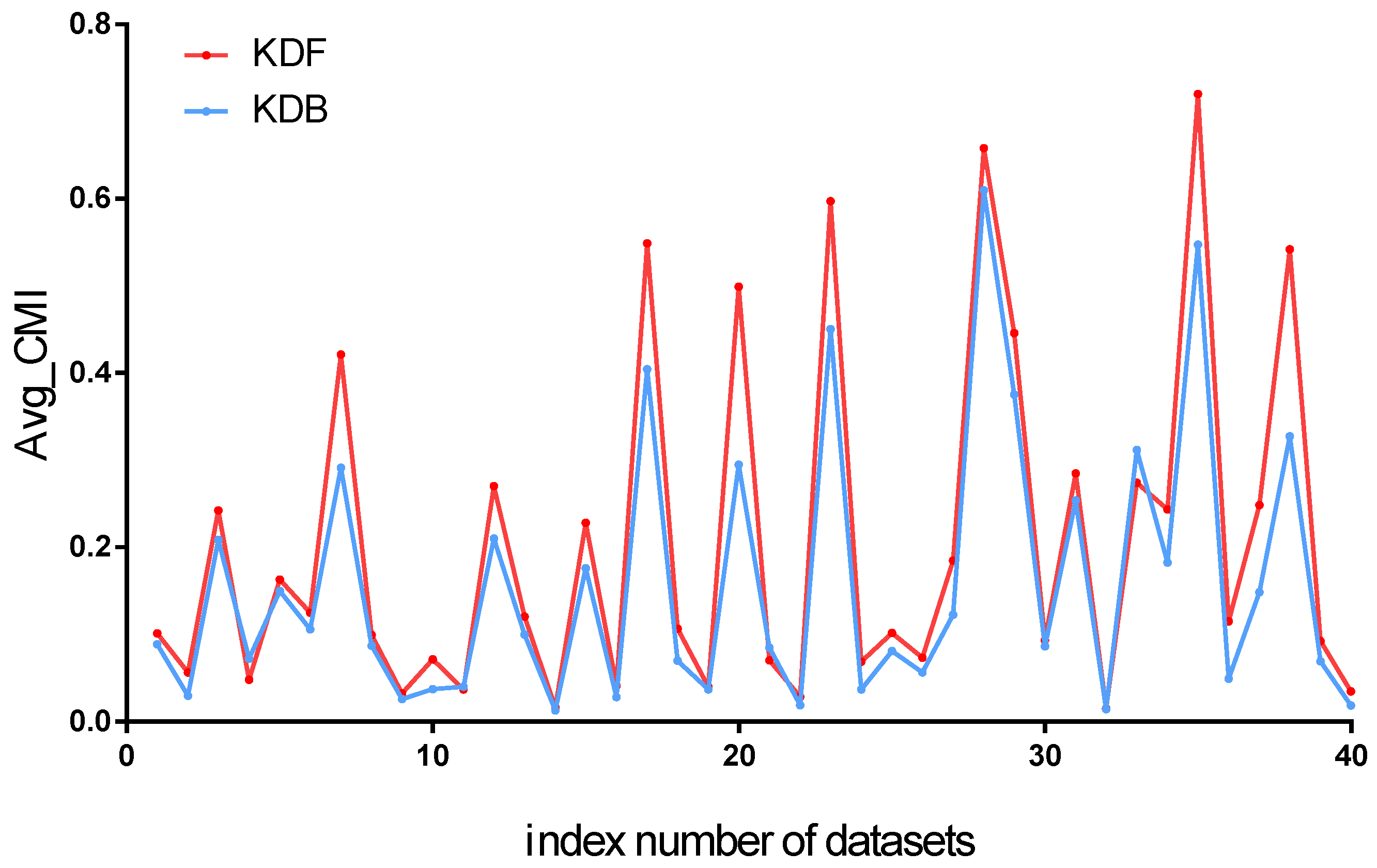
To show the superior performance of dependence analysis (i.e., the selection of ancestor attributes) of the KDF, we clarify from the viewpoint of conditional mutual information , which can be used to quantitatively evaluate the conditional dependence between and given C. We propose the definition of average conditional mutual information, that is, , to measure the intensity of conditional dependence between predictive attributes for the classifier. is defined as follows:
where is the parent of , and is the sum of numbers of arcs between predictive attributes. The comparison results of between KDF and KDB are shown in Figure 8. We can find that KDF has a significant advantage over KDB for almost all the datasets. According to Figure 8, we can see that the W/D/L of KDF against KDB is 35/1/4. That is to say, KDB has a higher value of than KDF on only four datasets. The experimental results prove that the selection of ancestor attributes of the KDF can fully demonstrate conditional dependence between predictive attributes; for example, the value of increases from 0.2947 to 0.4991 for the Vowel dataset.
4.3. Further Experimental Analysis
This part of the experiments compared the KDF with the out-of-core classifiers described in Section 4 in terms of zero-one loss. According to the zero-one loss results in Table A1 in Appendix A, we present summaries of W/D/L records in Table 3. When the dependence complexity increases, the performance of TAN and the KDB becomes better than that of NB. The two-dependence relationship helps the KDB to achieve a slightly better performance than TAN (16 wins and 13 losses). It is clear that AODE performs far better than NB (27 wins and 4 losses). However, the ensemble mechanism does not help ATAN to achieve superior performance to TAN (2 wins and 1 loss). The KDF performs the best. For example, when compared with the KDB, the KDF wins on 23 datasets and loses on 5 datasets. This advantage is more apparent when comparing the KDF with ATAN (26 wins and 2 losses). The KDF also provides better classification performance than AODE (26 wins and 5 losses).
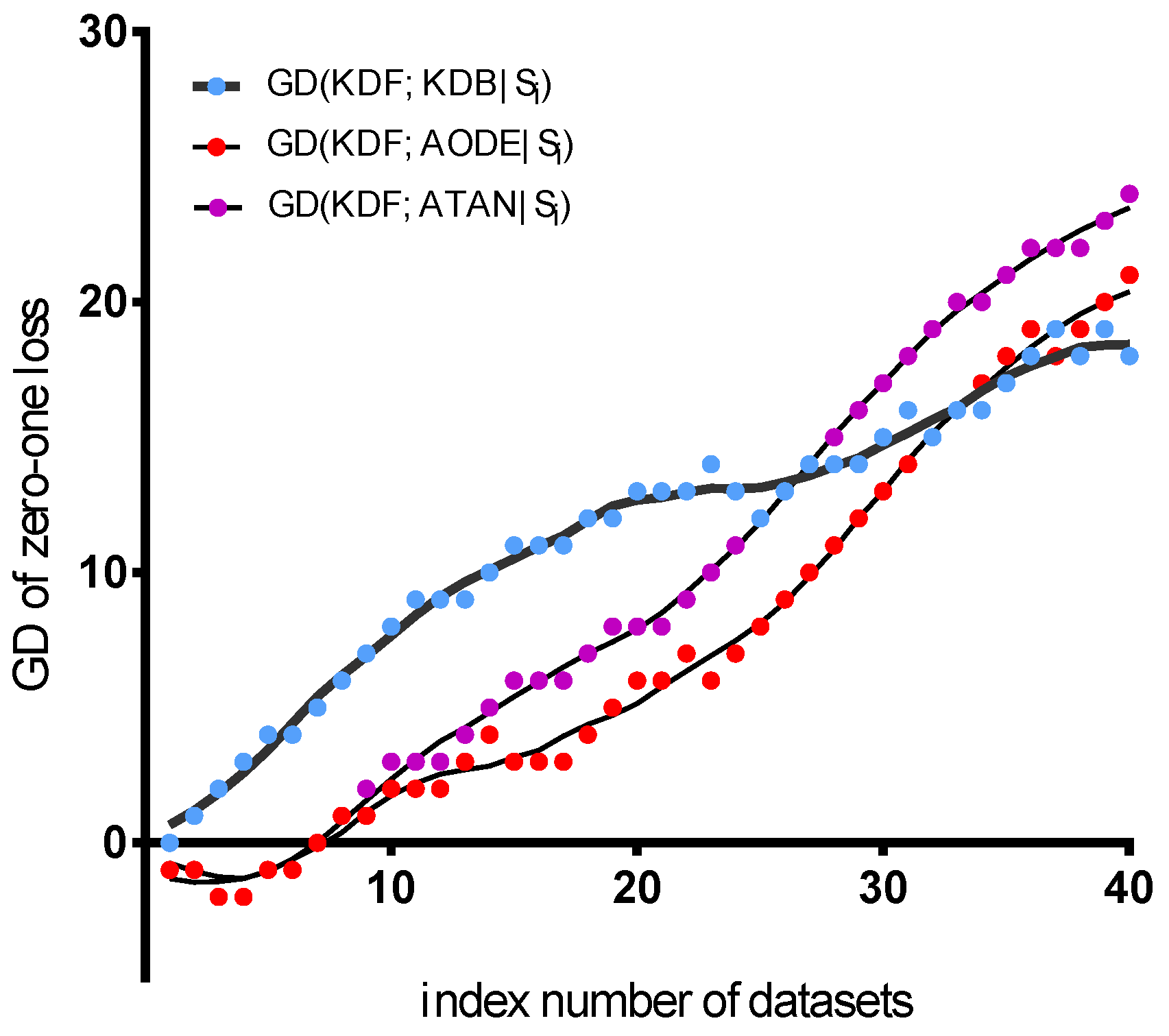
To clarify from the viewpoints of the ensemble mechanism and structure complexity, we only compare the KDF with three classifiers, that is, KDB, ATAN and AODE. We present the fitting curve of GD in terms of zero-one loss in Figure 9. Given datasets , the X-axis in Figure 9 represents the index number of datasets, and the Y-axis represents the value of , where is the collection of datasets for experimental study. In the following discussion, we first compare the KDF with other two ensemble classifiers, that is, ATAN and AODE. Then, the KDF is compared with the KDB in the case of the same value of k. As shown in Figure 9, the KDF only performs a little worse than ATAN when dealing with small datasets with less than 131 instances, for example, Echocardiogram. This indicates that fewer instances are not enough to support discovering significant dependencies for the KDF. However, as more instances are utilized for the training classifier, the sorting method of the KDF and the higher value of k will help to ensure that more dependencies will appear and be expressed in the joint probability distribution. This makes the KDF perform much better than ATAN (the maximum value of is 24). Owing to the same reason, the fitting curve of has a similar trend compared with the fitting curve of . When we compare the KDF with the KDB, the fitting curve shows a different trend. It is clear from Figure 9 that the KDF always performs much better than the KDB on datasets of different scale. This superior performance is due to the ensemble mechanism of the KDF. The KDF has n subclassifiers, where n is the number of predictive attributes, and each subclassifier of the KDF reflects almost the same quantities of mutual dependencies and conditional dependencies compared with the KDB. Moreover, diversity among the subclassifiers of the KDF is also a key part in the superior performance of the KDF. In order to prove this point, we show the results of average entropy diversity in the following discussion.
For the purpose of calculating the average entropy diversity of the KDF over datasets of a different scale and simultaneously ensuring the consistency of the data distribution, we take the Poker hand dataset as an example. Before the segmentation, 200 instances were selected as a test set and the remaining instances were for training. The training set is divided into 17 parts of different sizes. The scale of these 17 parts is in an exponential growth of 2 (from to ). Figure 10a shows the fitting curve of average entropy diversity of the KDF on the Poker hand dataset. As can be seen, there is a strong diversity among the subclassifiers of the KDF, and the maximum value is close to 0.48 when the dataset contains less than instances (4096 instances). The reason for this result is that fewer training instances make each subclassifier learn diverse mutual dependencies and conditional dependencies. As the quantities of instance increase, each subclassifier can be trained well and tends to vote for the same label. Therefore, the fitting curve of the average entropy diversity has a downward trend. However, the slight decrease in diversity does not produce a bad performance in classification accuracy. Figure 10b shows the corresponding fitting curve of zero-one loss of the KDF. We can find that as more instances are utilized for training, the KDF still achieves better classification performance in terms of zero-one loss.
4.3.1. Comparison with In-Core Random Forest
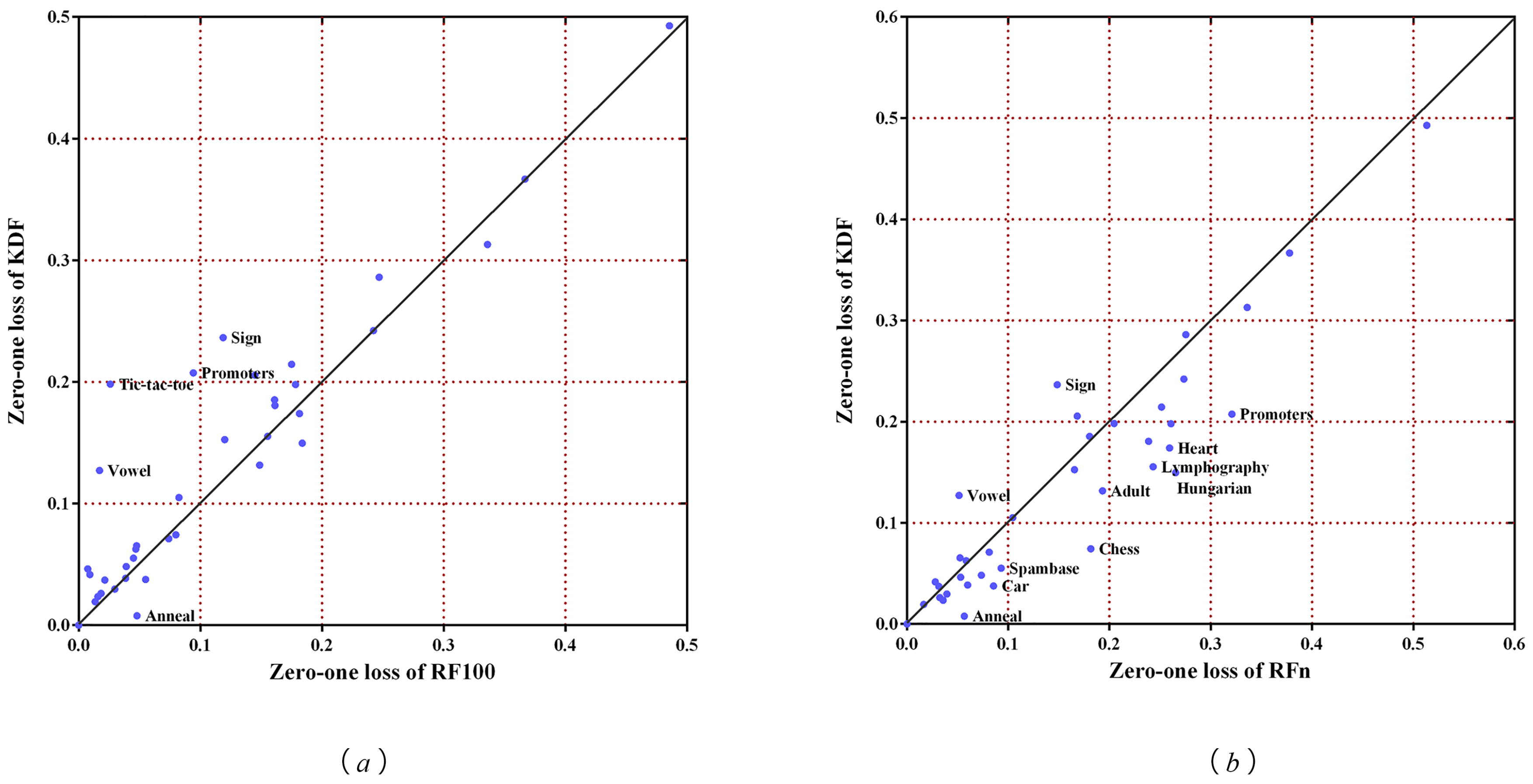
A random forest (RF) is a powerful in-core learning algorithm that is state-of-the-art. To further illustrate the performance of the KDF, here we first compare the KDF with the RF, which contains 100 trees (RF100) with respect to zero-one loss. From Table A1 in Appendix A, we can see that RF100 seems to perform better than the KDF on several datasets. In order to know how much RF100 wins by, we present the scatter plot in Figure 11a, where the X-axis represents the zero-one loss results of RF100 and the Y-axis represents the zero-one loss results of the KDF. We note that we do not obtain the results for RF100 on such two datasets as Covtype and Poker hand because of the limited memory; thus we remove these two points in the plot. We can see that the dataset Anneal is under the diagonal line, which means the KDF could beat RF100 on the Anneal dataset. Except for Vowel, Tic-tac-toe, Promoters and Sign, the other datasets fall close to the diagonal line. This means the performance of the KDF is close to the performance of RF100 on most datasets. It is worthwhile to keep in mind that the number of subclassifiers of the KDF (the maximum number is 64 on the Optdigits dataset) is much smaller than that of RF100.
It is unfair to make a comparison between the KDF and RF when they have a different number of subclassifiers. Thus we present another experiment that limits the RF with n trees (RFn), just as for KDF. Table A1 in Appendix A presents the zero-one loss in detail. We also present the scatter plot in Figure 11b, where the X-axis represents the zero-one loss results of RFn and the Y-axis represents the zero-one loss results of the KDF. From Figure 11b, we can easily find that most datasets are under the diagonal line, for example, Anneal, Car, Chess, Hungarian, Promoters, and so on, which means the KDF performs much better than RFn on these datasets. Except for Vowel and Sign, the other datasets fall close to the diagonal line, which means the performance of the KDF is close to that of RFn on the remaining datasets. The superior performance of the RF can be partially attributed to the great number of decision trees. The experiment results show that the KDF is competitive with the RF when they contain the same number of subclassifiers.
4.3.2. Bias Results
Bias can be used to evaluate the extent to which the final model learned from training data fits the entire dataset. To further illustrate the performance of the proposed KDF, the experimental results of average bias are shown in Table A2 in Appendix A. Only 18 large datasets (size > 2310) are selected for comparison because of statistical significance. Table 4 shows the corresponding W/D/L records. From Table 4, we can see that the fitness of NB is the poorest because its structure is definite regardless of the true data distribution. Although the structure of AODE is also definite, it shows a great advantage over NB (17 wins). The main reason may be that it averages all models from a restricted class of one-dependence classifiers and reflects more dependencies between predictive attributes. ATAN and TAN almost have the same bias results (18 draws). The KDF still performs the best, although the advantage is not significant. By sorting attributes and training n subclassifiers, the ensemble mechanism can help the KDF make full use of the information that is supplied by the training data. The complicated relationship among attributes are measured and depicted from the viewpoint of information theory. Thus, performance robustness can be achieved. The W/D/L records of the KDF compared to AODE show that the advantage is obvious (11 wins and 4 losses) for bias. We can also find that more often than not, the KDF obtains lower bias than ATAN (8 wins and 4 losses) and the KDB (7 wins and 5 losses).
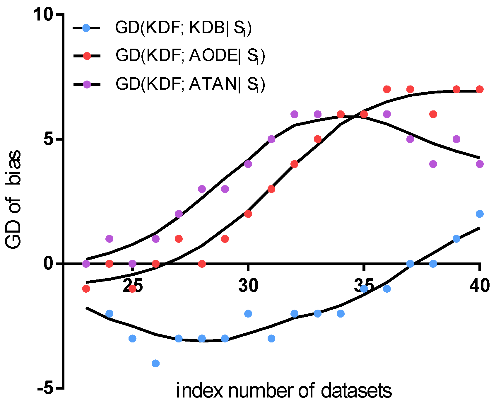
Figure 12 shows the fitting curve of GD in terms of bias. The results indicate that the KDF is competitive to AODE (the minimum value of is and the maximum value of is 7). We believe the reason for the KDF performing better is that the sorting method means it reflect more dependencies than AODE. The KDF performs much better than ATAN (the maximum value of is 6) when dealing with relatively small datasets containing less than 67,557 instances, for example, the Connect-4 dataset. As the quantities of instance increase, dependencies between predictive attributes are completely represented, and the final structure of both the KDF and ATAN fits the entire dataset well. Thus, the KDF wins on two out of the last four datasets. The comparison results between the KDF and KDB in terms of show another trend. From the fitting curve, we can find that the KDB is competitive to the KDF for the first four datasets, which contain less than 4601 instances. The minimum value of is as low as . The reason for this result is that KDF cannot discover enough dependencies when the dataset contains lower quantities of data. As the quantities of instance increase, the KDF achieves greater advantage in terms of bias.
4.3.3. Variance Results
Table A3 in Appendix A shows the experimental results of average variance on 18 large datasets. Table 5 shows corresponding W/D/L records. A higher degree of attribute dependence means more parameters, which increases the risk of overfitting. An overfitted model does not perform well on data outside the training data. It is clear that NB performs the best among these algorithms, because its network structure is definite and is therefore insensitive to changes in the training set, as shown in Table 5. Owing to the same reason, AODE also has a competitive performance. ATAN has almost the same performance (17 draws) compared to TAN. By contrast, the KDB performs the worst. When the value of k increases, the resulting network tends to have a complex structure. The KDF wins on 13 out of 18 datasets compared to the KDB. AODE wins over the KDF, although the advantage is not significant (7 wins and 9 losses).
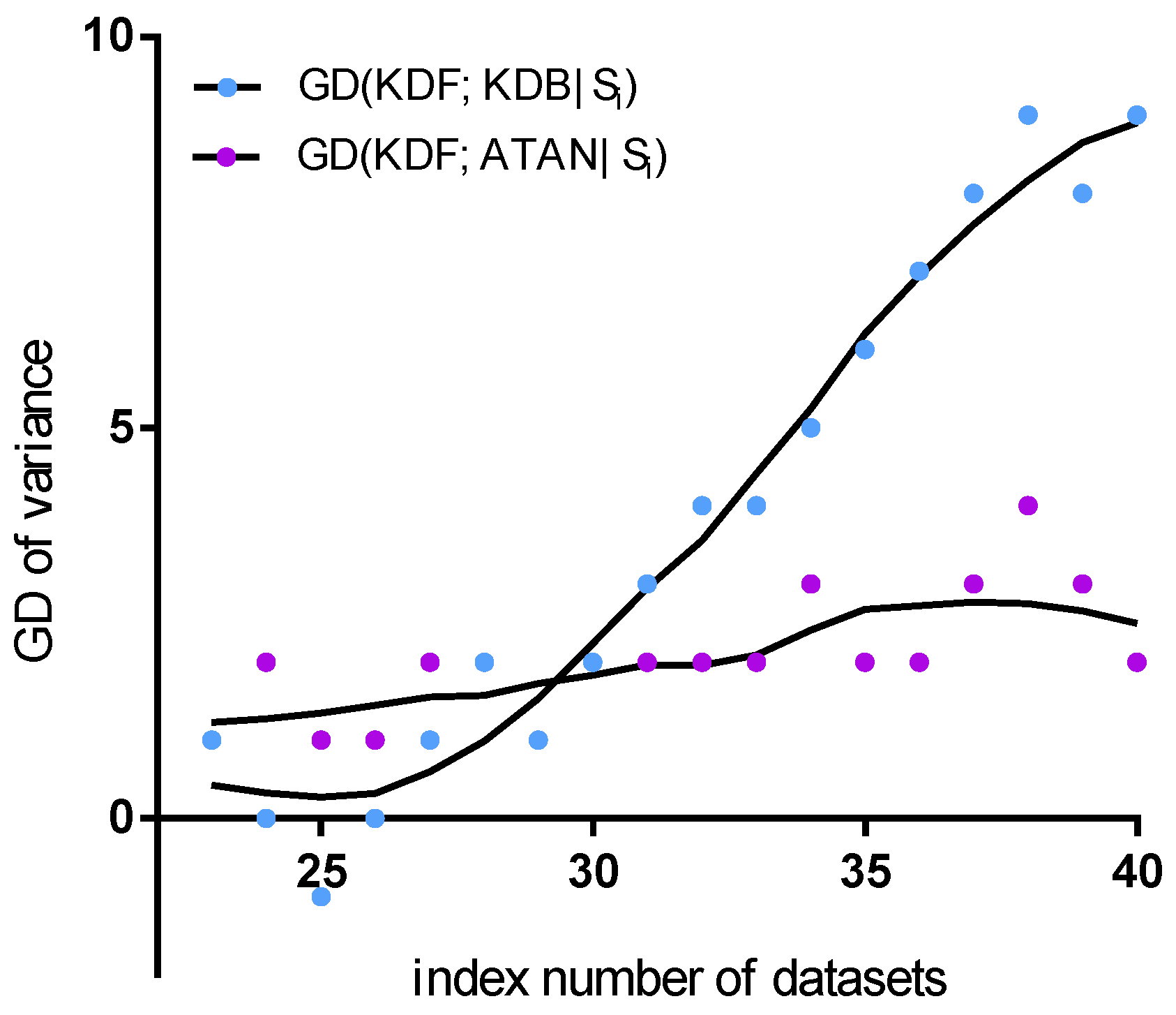
Figure 13 shows the fitting curve of GD of in terms of variance. NB and AODE are neglected, because they are insensitive to the changes in the training set. TAN is not considered, because of almost the same performance as ATAN. The KDF obtains a significant advantage over the KDB, but performs similarly to ATAN. ATAN can only represent the most significant one-dependence relationships between attributes and thus performs similarly to TAN. The ensemble mechanism helps the KDF fully represent many non-significant dependencies. This may be the main reason why ATAN and the KDF are not sensitive to the changes in data distribution. In contrast, although the KDB can also represent significant dependencies, some non-significant dependencies will be affected by the training data, particularly when the dataset size is relatively large.
5. Conclusions
The KDB delivers fast and effective classification with a clear theoretical foundation. The current work is motivated by the desire to obtain the accuracy improvements derived by the sorting method and ensemble mechanism. Our new classification technique averages all models from a restricted class of k-dependence classifiers, the class of all such classifiers that have a diverse network structure depending on a different attribute order. Our experiments have shown its superiority from the comparison results of zero-one loss, bias, variance and diversity. However, the subclassifiers of the KDF are trained using the same training set, which may lead to overfitting. Moreover, the number of subclassifiers of the KDF is determined by the number of predictive attributes and is not as many as for the RF. In all, we believe that we have been successful in our goal of developing a classification learning technique that retains the direct theoretical foundation of the KDB while fully representing conditional dependencies among attributes.
Acknowledgments
This work was supported by the National Science Foundation of China (Grant No. 61272209) and the Agreement of Science & Technology Development Project, Jilin Province (No. 20150101014JC).
Author Contributions
All authors have contributed to the study and to the preparation of the article. They have read and approved the final manuscript.
Conflicts of Interest
The authors declare no conflict of interest.
Appendix A. Tables of the Experimental Section

Table A1.
Experimental results of average zero-one loss.
| Dataset | NB | TAN | AODE | KDB | ATAN | RF100 | RFn | KDB | KDF |
|---|---|---|---|---|---|---|---|---|---|
| Post-operative | 0.3444 | 0.3667 | 0.3333 | 0.3778 | 0.3667 | 0.3667 | 0.3778 | 0.3667 | 0.3667 |
| Zoo | 0.0297 | 0.0099 | 0.0297 | 0.0495 | 0.0198 | 0.0297 | 0.0396 | 0.0396 | 0.0297 |
| Promoters | 0.0755 | 0.1321 | 0.1321 | 0.2547 | 0.1226 | 0.0943 | 0.3208 | 0.2453 | 0.2075 |
| Echocardiogram | 0.3359 | 0.3282 | 0.3206 | 0.3435 | 0.3282 | 0.3359 | 0.3359 | 0.3130 | 0.3130 |
| Lymphography | 0.1486 | 0.1757 | 0.1689 | 0.2365 | 0.1689 | 0.1554 | 0.2432 | 0.1757 | 0.1554 |
| Hepatitis | 0.1935 | 0.1677 | 0.1806 | 0.1871 | 0.1742 | 0.1613 | 0.2387 | 0.1290 | 0.1806 |
| Autos | 0.3122 | 0.2146 | 0.2049 | 0.2049 | 0.2146 | 0.1610 | 0.1805 | 0.2049 | 0.1854 |
| Glass-id | 0.2617 | 0.2196 | 0.2523 | 0.2196 | 0.2196 | 0.1449 | 0.1682 | 0.1963 | 0.2056 |
| Heart | 0.1778 | 0.1926 | 0.1704 | 0.2111 | 0.1926 | 0.1815 | 0.2593 | 0.2000 | 0.1741 |
| Hungarian | 0.1599 | 0.1701 | 0.1667 | 0.1803 | 0.1769 | 0.1837 | 0.2653 | 0.1667 | 0.1497 |
| Heart disease-c | 0.1815 | 0.2079 | 0.2013 | 0.2244 | 0.2046 | 0.1782 | 0.2607 | 0.2046 | 0.1980 |
| Ionosphere | 0.1054 | 0.0684 | 0.0741 | 0.0741 | 0.0684 | 0.0741 | 0.0813 | 0.0769 | 0.0712 |
| House votes-84 | 0.0943 | 0.0552 | 0.0529 | 0.0506 | 0.0529 | 0.0391 | 0.0736 | 0.0483 | 0.0483 |
| Chess | 0.1125 | 0.0926 | 0.0998 | 0.0998 | 0.0926 | 0.0799 | 0.1815 | 0.0780 | 0.0744 |
| Breast cancer-w | 0.0258 | 0.0415 | 0.0358 | 0.0744 | 0.0415 | 0.0386 | 0.0601 | 0.0815 | 0.0386 |
| Pima-Ind diabetes | 0.2448 | 0.2383 | 0.2383 | 0.2448 | 0.2370 | 0.2422 | 0.2734 | 0.2500 | 0.2422 |
| Vehicle | 0.3924 | 0.2943 | 0.2896 | 0.2943 | 0.2943 | 0.2470 | 0.2754 | 0.2872 | 0.2861 |
| Anneal | 0.0379 | 0.0111 | 0.0089 | 0.0089 | 0.0111 | 0.0479 | 0.0568 | 0.0089 | 0.0078 |
| Tic-tac-toe | 0.3069 | 0.2286 | 0.2651 | 0.2035 | 0.2276 | 0.0261 | 0.2046 | 0.2004 | 0.1983 |
| Vowel | 0.4242 | 0.1303 | 0.1495 | 0.1818 | 0.1263 | 0.0172 | 0.0515 | 0.1616 | 0.1273 |
| Contraceptive-mc | 0.5037 | 0.4888 | 0.4942 | 0.5003 | 0.4895 | 0.4854 | 0.5132 | 0.5003 | 0.4929 |
| Car | 0.1400 | 0.0567 | 0.0816 | 0.0382 | 0.0567 | 0.0550 | 0.0856 | 0.0492 | 0.0376 |
| Segment | 0.0788 | 0.0390 | 0.0342 | 0.0472 | 0.0398 | 0.0216 | 0.0316 | 0.0476 | 0.0372 |
| Kr vs. kp | 0.1214 | 0.0776 | 0.0842 | 0.0416 | 0.0776 | 0.0075 | 0.0532 | 0.0795 | 0.0463 |
| Sick | 0.0308 | 0.0257 | 0.0273 | 0.0223 | 0.0255 | 0.0159 | 0.0358 | 0.0276 | 0.0236 |
| Spambase | 0.1015 | 0.0669 | 0.0672 | 0.0635 | 0.0669 | 0.0450 | 0.0932 | 0.0700 | 0.0552 |
| Optdigits | 0.0767 | 0.0407 | 0.0311 | 0.0372 | 0.0404 | 0.0185 | 0.0326 | 0.0372 | 0.0262 |
| Satellite | 0.1806 | 0.1214 | 0.1148 | 0.1080 | 0.1209 | 0.0825 | 0.1046 | 0.1103 | 0.1051 |
| Mushrooms | 0.0196 | 0.0001 | 0.0001 | 0.0000 | 0.0001 | 0.0000 | 0.0002 | 0.0000 | 0.0000 |
| Thyroid | 0.1111 | 0.0720 | 0.0701 | 0.0706 | 0.0719 | 0.0477 | 0.0525 | 0.0794 | 0.0654 |
| Sign | 0.3586 | 0.2755 | 0.2821 | 0.2539 | 0.2755 | 0.1187 | 0.1485 | 0.2473 | 0.2365 |
| Nursery | 0.0973 | 0.0654 | 0.0730 | 0.0289 | 0.0655 | 0.0093 | 0.0281 | 0.0586 | 0.0416 |
| Magic | 0.2239 | 0.1675 | 0.1752 | 0.1637 | 0.1674 | 0.1200 | 0.1655 | 0.1656 | 0.1526 |
| Adult | 0.1592 | 0.1380 | 0.1493 | 0.1383 | 0.1380 | 0.1487 | 0.1931 | 0.1350 | 0.1317 |
| Shuttle | 0.0039 | 0.0015 | 0.0008 | 0.0009 | 0.0013 | 0.0001 | 0.0002 | 0.0007 | 0.0007 |
| Connect-4 | 0.2783 | 0.2354 | 0.2420 | 0.2283 | 0.2354 | 0.1751 | 0.2515 | 0.2380 | 0.2145 |
| Waveform | 0.0220 | 0.0202 | 0.0180 | 0.0256 | 0.0202 | 0.0136 | 0.0168 | 0.0197 | 0.0195 |
| Census income | 0.2363 | 0.0628 | 0.1004 | 0.0508 | 0.0628 | 0.0470 | 0.0587 | 0.0526 | 0.0626 |
| Covtype | 0.3158 | 0.2517 | 0.2389 | 0.1421 | 0.2516 | − | − | 0.1311 | 0.1291 |
| Poker hand | 0.4988 | 0.3295 | 0.4812 | 0.1961 | 0.3295 | − | − | 0.2254 | 0.2204 |
NB, standard naive Bayes. TAN, tree-augmented naive Bayes. AODE, averaged one-dependence estimator. KDB, k-dependence Bayesian classifier. KDB, the KDB that only performs the sorting method proposed above. ATAN, averaged tree-augmented naive Bayes. RF100, random forest containing 100 trees. RFn, random forest containing n trees, where n is the number of predictive attributes. KDF, k-dependence forest.
Table A2.
Experimental results of bias on large datasets.
| Dataset | NB | TAN | AODE | KDB | ATAN | KDF |
|---|---|---|---|---|---|---|
| Segment | 0.0857 | 0.0454 | 0.0393 | 0.0392 | 0.0450 | 0.0434 |
| Kr vs. kp | 0.1105 | 0.0668 | 0.0699 | 0.0390 | 0.0669 | 0.0450 |
| Sick | 0.0232 | 0.0228 | 0.0242 | 0.0208 | 0.0223 | 0.0291 |
| Spambase | 0.0965 | 0.0656 | 0.0669 | 0.0504 | 0.0658 | 0.0558 |
| Optdigits | 0.0655 | 0.0308 | 0.0295 | 0.0285 | 0.0306 | 0.0241 |
| Satellite | 0.1661 | 0.0941 | 0.0801 | 0.0810 | 0.0941 | 0.0849 |
| Mushrooms | 0.0399 | 0.0002 | 0.0010 | 0.0002 | 0.0002 | 0.0002 |
| Thyroid | 0.1014 | 0.0749 | 0.0664 | 0.0751 | 0.0734 | 0.0593 |
| Sign | 0.3109 | 0.2464 | 0.2500 | 0.2154 | 0.2455 | 0.2316 |
| Nursery | 0.0729 | 0.0507 | 0.0519 | 0.0418 | 0.0512 | 0.0367 |
| Magic | 0.1987 | 0.1357 | 0.1613 | 0.1321 | 0.1356 | 0.1370 |
| Adult | 0.1485 | 0.1125 | 0.1182 | 0.1135 | 0.1124 | 0.1099 |
| Shuttle | 0.0066 | 0.0023 | 0.0023 | 0.0028 | 0.0023 | 0.0023 |
| Connect-4 | 0.2327 | 0.1829 | 0.1921 | 0.1788 | 0.1830 | 0.1798 |
| Waveform | 0.0314 | 0.0138 | 0.0151 | 0.0180 | 0.0138 | 0.0146 |
| Census income | 0.1271 | 0.0513 | 0.0499 | 0.0541 | 0.0500 | 0.0532 |
| Covtype | 0.2288 | 0.2257 | 0.2148 | 0.2238 | 0.2259 | 0.1309 |
| Poker hand | 0.3266 | 0.2265 | 0.2627 | 0.3306 | 0.2267 | 0.2684 |
Table A3.
Experimental results of variance on large datasets.
| Dataset | NB | TAN | AODE | KDB | ATAN | KDF |
|---|---|---|---|---|---|---|
| Segment | 0.0173 | 0.0212 | 0.0179 | 0.0261 | 0.0211 | 0.0172 |
| Kr vs. kp | 0.0249 | 0.0185 | 0.0233 | 0.0101 | 0.0184 | 0.0128 |
| Sick | 0.0058 | 0.0068 | 0.0045 | 0.0056 | 0.0065 | 0.0087 |
| Spambase | 0.0104 | 0.0171 | 0.0139 | 0.0238 | 0.0169 | 0.0171 |
| Optdigits | 0.0247 | 0.0280 | 0.0236 | 0.0322 | 0.0279 | 0.0243 |
| Satellite | 0.0207 | 0.0413 | 0.0491 | 0.0529 | 0.0413 | 0.0400 |
| Mushrooms | 0.0081 | 0.0006 | 0.0003 | 0.0005 | 0.0006 | 0.0007 |
| Thyroid | 0.0357 | 0.0388 | 0.0411 | 0.0368 | 0.0389 | 0.0340 |
| Sign | 0.0786 | 0.0779 | 0.0974 | 0.0966 | 0.0784 | 0.0789 |
| Nursery | 0.0270 | 0.0380 | 0.0295 | 0.0447 | 0.0377 | 0.0376 |
| Magic | 0.0409 | 0.0792 | 0.0613 | 0.0818 | 0.0794 | 0.0805 |
| Adult | 0.0355 | 0.0640 | 0.0446 | 0.0717 | 0.0634 | 0.0555 |
| Shuttle | 0.0038 | 0.0008 | 0.0021 | 0.0021 | 0.0009 | 0.0010 |
| Connect-4 | 0.0953 | 0.0883 | 0.1103 | 0.1044 | 0.0881 | 0.0873 |
| Waveform | 0.0044 | 0.0119 | 0.0068 | 0.0102 | 0.0118 | 0.0086 |
| Census income | 0.0468 | 0.0223 | 0.0477 | 0.0226 | 0.0224 | 0.0200 |
| Covtype | 0.1232 | 0.1665 | 0.1329 | 0.1623 | 0.1752 | 0.1887 |
| Poker hand | 0.2091 | 0.2311 | 0.2141 | 0.3284 | 0.2305 | 0.2693 |
References
- Zhou, L.P.; Wang, L.; Liu, L.Q.; Ogunbona, P.; Shen, D.G. Learning Discriminative Bayesian networks from high-dimensional continuous neuroimaging data. IEEE Trans. Pattern Anal. Mach. Intell. 2015, 38, 2269–2283. [Google Scholar] [CrossRef] [PubMed]
- Pernkopf, F.; Wohlmayr, M.; Tschiatschek, S. Maximum margin Bayesian network classifiers. IEEE Trans. Pattern Anal. Mach. Intell. 2012, 34, 521–532. [Google Scholar] [CrossRef] [PubMed]
- Pernkopf, F.; Bilmes, J. Efficient heuristics for discriminative structure learning of Bayesian network classifiers. J. Mach. Learn. Res. 2010, 11, 2323–2360. [Google Scholar]
- Carvalho, A.; Adão, P.; Mateus, P. Efficient approximation of the conditional relative entropy with applications to discriminative learning of Bayesian network classifiers. Entropy 2013, 15, 2716–2735. [Google Scholar] [CrossRef]
- Wang, S.C.; Gao, R.; Wang, L.M. Bayesian network classifiers based on Gaussian kernel density. Expert Syst. Appl. 2016, 51, 207–217. [Google Scholar] [CrossRef]
- He, Y.L.; Wang, R.; Kwong, S.; Wang, X.Z. Bayesian classifiers based on probability density estimation and their applications to simultaneous fault diagnosis. Inf. Sci. 2014, 259, 252–268. [Google Scholar] [CrossRef]
- Varando, G.; Bielza, C.; Larrañaga, P. Decision boundary for discrete Bayesian network classifiers. J. Mach. Learn. Res. 2015, 16, 2725–2749. [Google Scholar]
- Martinez, A.M.; Webb, G.I.; Chen, S.L.; Nayyar, A.Z. Scalable learning of Bayesian network classifiers. J. Mach. Learn. Res. 2013, 1, 1–30. [Google Scholar]
- Bielza, C.; Larranaga, P. Discrete Bayesian Network Classifiers: A Survey. ACM Comput. Surv. 2014, 47, 1–43. [Google Scholar] [CrossRef]
- Friedman, N.; Dan, G.; Goldszmidt, M. Bayesian classifiers. Mach. Learn. 1997, 29, 131–163. [Google Scholar] [CrossRef]
- Sahami, M. Learning limited dependence Bayesian classifiers. In Proceedings of the Second International Conference on Knowledge Discovery and Data Mining, Portland, OR, USA, 2–4 August 1996; pp. 335–338. [Google Scholar]
- Chen, S.L.; Martinez, A.M.; Webb, G.I.; Wang, L.M. Selective AnDE for large data learning: A low-bias memory constrained approach. Knowl. Inf. Syst. 2017, 50, 1–29. [Google Scholar] [CrossRef]
- Chen, S.L.; Martinez, A.M.; Webb, G.I.; Wang, L.M. Sample-based attribute selective AnDE for large data. IEEE Trans. Knowl. Data. Eng. 2016, 29, 1–14. [Google Scholar]
- Webb, G.I.; Boughton, J.R.; Wang, Z. Not so naive Bayes: Aggregating one-dependence estimators. Mach. Learn. 2005, 58, 5–24. [Google Scholar] [CrossRef]
- Jiang, L.X.; Cai, Z.H.; Wang, D.H.; Zhang, H. Improving tree augmented naive bayes for class probability estimation. Knowl.-Based Syst. 2012, 26, 239–245. [Google Scholar] [CrossRef]
- Pearl, J. Probabilistic Reasoning in Intelligent Systems: Networks of Plausible Inference; Morgan Kaufmann: Burlington, MA, USA, 1988. [Google Scholar]
- Jiang, S.; Zhang, H. Full Bayesian network classifiers. In Proceedings of the 23rd International Conference on Machine Learning, Pittsburgh, PA, USA, 25–29 June 2006; pp. 897–904. [Google Scholar]
- Dagum, P.; Luby, M. Approximating Probabilistic Inference in Bayesian Belief Networks is NP-Hard. Artif. Intell. 1993, 60, 141–153. [Google Scholar] [CrossRef]
- Zhao, Y.P.; Chen, Y.T.; Tu, K.W.; Tian, J. Learning Bayesian network structures under incremental construction curricula. Neurocomputing 2017, 258, 30–40. [Google Scholar] [CrossRef]
- Wu, J.; Cai, Z. A naive Bayes probability estimation model based on self-adaptive differential evolution. J. Intell. Inf. Syst. 2014, 42, 671–694. [Google Scholar] [CrossRef]
- Francisco, L.; Anderson, A. Bagging k-dependence probabilistic networks: An alternative powerful fraud detection tool. Expert Syst. Appl. 2012, 39, 11583–11592. [Google Scholar]
- Domingos, P.; Pazzani, M. On the optimality of the simple Bayesian classifier under zero-one loss. Mach. Learn. 1997, 29, 103–130. [Google Scholar] [CrossRef]
- Chow, C.K.; Liu, C.N. Approximating discrete probability distributions dependence trees. IEEE Trans. Inf. Theory. 1968, 14, 462–467. [Google Scholar] [CrossRef]
- Madden, M.G. On the classification performance of TAN and general Bayesian networks. Knowl.-Based Syst. 2009, 22, 489–495. [Google Scholar] [CrossRef]
- Ruz, G.A.; Pham, D.T. Building Bayesian network classifiers through a Bayesian complexity monitoring system. Proc. Inst. Mech. Eng. Part C J. Mech. Eng. Sci. 2009, 223, 743–755. [Google Scholar] [CrossRef]
- Webb, G.I.; Boughton, J.; Zheng, F.; Ting, K.M.; Salem, H. Learning by extrapolation from marginal to full-multivariate probability distributions: Decreasingly naive Bayesian classification. Mach. Learn. 2012, 86, 233–272. [Google Scholar] [CrossRef]
- Murphy, P.M.; Aha, D.W. UCI Repository of Machine Learning Databases. Available online: http://www.ics.uci.edu/~mlearn/MLRepository.html (accessed on 28 November 2017).
- Fayyad, U.M.; Irani, K.B. Multi-interval Discretization of Continuous-Valued Attributes for Classification Learning. In Proceedings of the 13th International Joint Conference on Artificial Intelligence, Chambery, France, 28 August–3 September 1993; pp. 1022–1029. [Google Scholar]
- Kohavi, R.; Wolpert, D. Bias Plus Variance Decomposition for Zero-One Loss Functions. In Proceedings of the Thirteenth International Conference on Machine Learning, Bari, Italy, 3–6 July 1996; pp. 275–283. [Google Scholar]
Figure 1.
(a) The proportional distribution of conditional mutual information ; (b) the proportional distribution of mutual information . The predictive attributes of Car are represented by .
Figure 1.
(a) The proportional distribution of conditional mutual information ; (b) the proportional distribution of mutual information . The predictive attributes of Car are represented by .
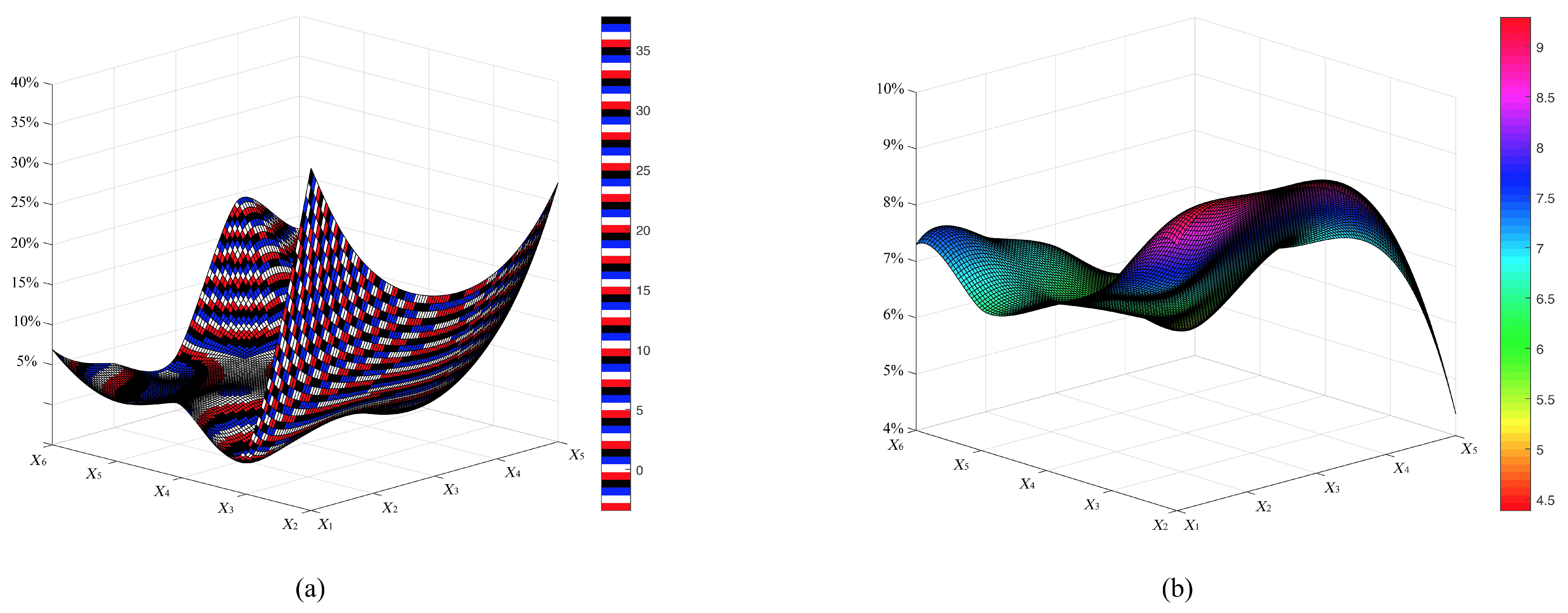
Figure 2.
(a) An example of naive Bayes (NB); (b) an example of averaged one-dependence estimator (AODE).
Figure 2.
(a) An example of naive Bayes (NB); (b) an example of averaged one-dependence estimator (AODE).

Figure 3.
(a) An example of tree-augmented naive Bayes (TAN), which takes as the root node; (b) a subclassifier of averaged TAN (ATAN), which takes as the root node.
Figure 3.
(a) An example of tree-augmented naive Bayes (TAN), which takes as the root node; (b) a subclassifier of averaged TAN (ATAN), which takes as the root node.

Figure 4.
An example of k-dependence Bayesian classifier (KDB; k = 2).

Figure 5.
An example of the hierarchical dependency relationship.
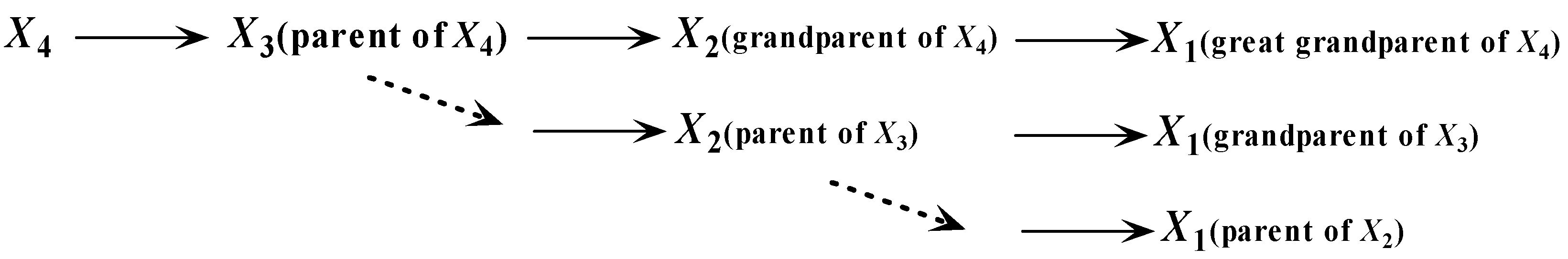
Figure 6.
(a) An exmple of a subclassifier of k-dependence forest (KDF) and supposing the predetermined attribute sequence is and . (b) The corresponding parent-child relationships.
Figure 6.
(a) An exmple of a subclassifier of k-dependence forest (KDF) and supposing the predetermined attribute sequence is and . (b) The corresponding parent-child relationships.
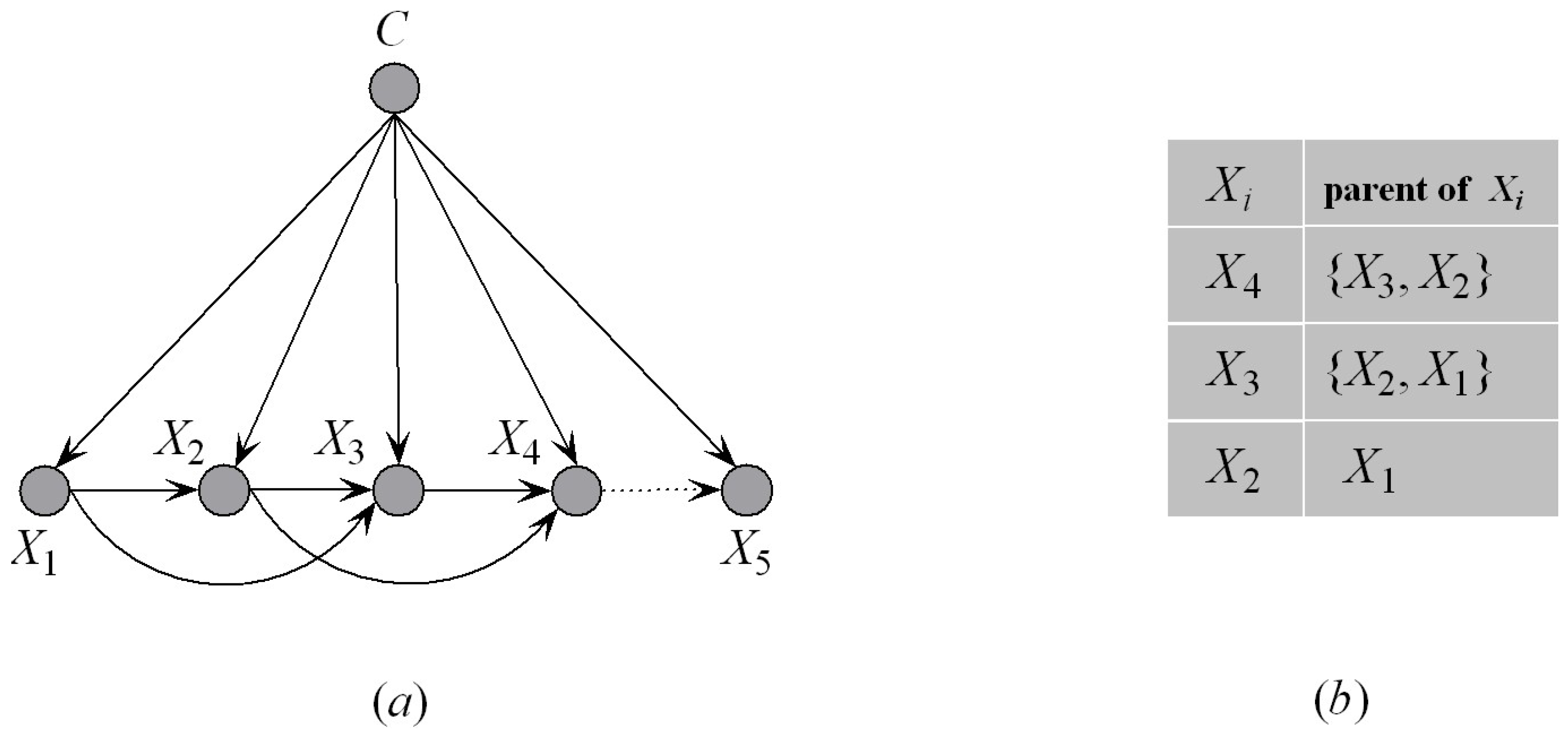
Figure 7.
The scatter plot of KDB and k-dependence Bayesian classifier (KDB) in terms of zero-one loss.
Figure 7.
The scatter plot of KDB and k-dependence Bayesian classifier (KDB) in terms of zero-one loss.
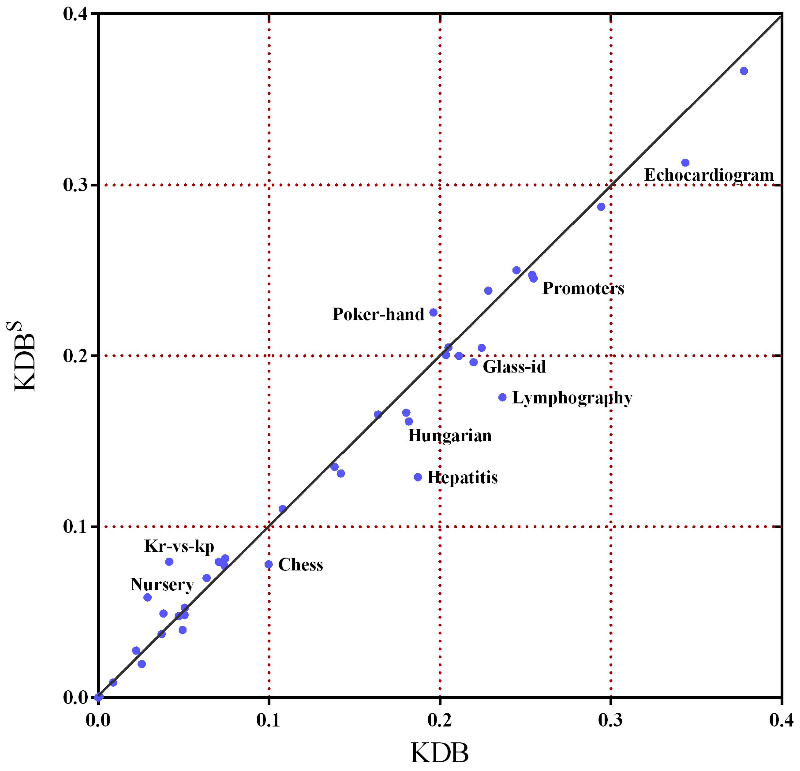
Figure 8.
The comparison results of between k-dependence forest (KDF) and k-dependence Bayesian classifier (KDB).
Figure 8.
The comparison results of between k-dependence forest (KDF) and k-dependence Bayesian classifier (KDB).

Figure 9.
The fitting curves of goal difference (GD) in terms of zero-one loss.

Figure 10.
The fitting curve of (a) average entropy diversity, and (b) zero-one loss of k-dependence forest (KDF) on Poker hand dataset.
Figure 10.
The fitting curve of (a) average entropy diversity, and (b) zero-one loss of k-dependence forest (KDF) on Poker hand dataset.
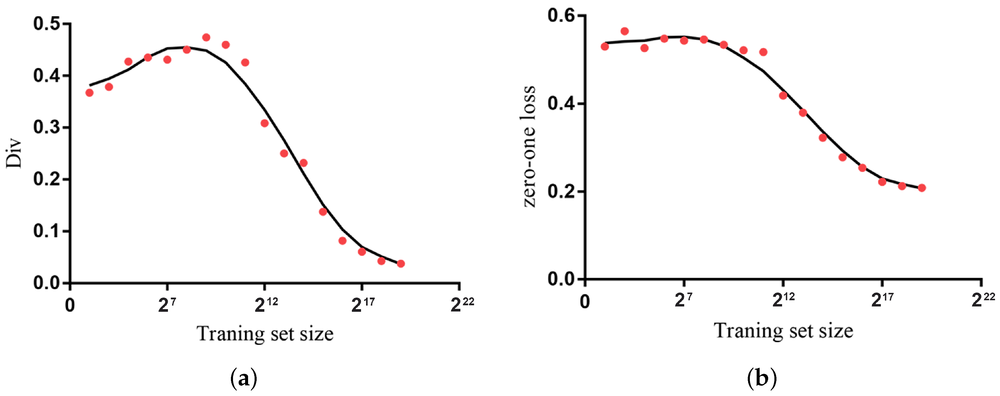
Figure 11.
The scatter plot of (a) k-dependence forest (KDF) and random forest 100 (RF100), and (b) KDF and random forest n (RFn) in terms of zero-one loss.
Figure 11.
The scatter plot of (a) k-dependence forest (KDF) and random forest 100 (RF100), and (b) KDF and random forest n (RFn) in terms of zero-one loss.

Figure 12.
The fitting curve of goal difference (GD) in terms of bias.

Figure 13.
The fitting curve of goal difference (GD) in terms of variance.

Table 1.
Datasets.
| Index | Dataset | # Instance | Attribute | Class | Index | Dataset | # Instance | Attribute | Class |
|---|---|---|---|---|---|---|---|---|---|
| 1 | Post-operative | 90 | 8 | 3 | 21 | Contraceptive-mc | 1473 | 9 | 3 |
| 2 | Zoo | 101 | 16 | 7 | 22 | Car | 1728 | 6 | 4 |
| 3 | Promoters | 106 | 57 | 2 | 23 | Segment | 2310 | 19 | 7 |
| 4 | Echocardiogram | 131 | 6 | 2 | 24 | Kr vs. kp | 3196 | 36 | 2 |
| 5 | Lymphography | 148 | 18 | 4 | 25 | Sick | 3772 | 29 | 2 |
| 6 | Hepatitis | 155 | 19 | 2 | 26 | Spambase | 4601 | 57 | 2 |
| 7 | Autos | 205 | 25 | 7 | 27 | Optdigits | 5620 | 64 | 10 |
| 8 | Glass-id | 214 | 9 | 3 | 28 | Satellite | 6435 | 36 | 6 |
| 9 | Heart | 270 | 12 | 2 | 29 | Mushrooms | 8124 | 22 | 2 |
| 10 | Hungarian | 294 | 13 | 2 | 30 | Thyroid | 9169 | 29 | 20 |
| 11 | Heart disease-c | 303 | 13 | 2 | 31 | Sign | 12,546 | 8 | 3 |
| 12 | Ionosphere | 351 | 34 | 2 | 32 | Nursery | 12,960 | 8 | 5 |
| 13 | House votes-84 | 435 | 16 | 2 | 33 | Magic | 19,020 | 10 | 2 |
| 14 | Chess | 551 | 39 | 2 | 34 | Adult | 48,842 | 14 | 2 |
| 15 | Breast cancer-w | 699 | 9 | 2 | 35 | Shuttle | 58,000 | 9 | 7 |
| 16 | Pima-Ind diabetes | 768 | 8 | 2 | 36 | Connect-4 | 67,557 | 42 | 3 |
| 17 | Vehicle | 846 | 18 | 4 | 37 | Waveform | 100,000 | 21 | 3 |
| 18 | Anneal | 898 | 39 | 6 | 38 | Census income | 299,285 | 41 | 2 |
| 19 | Tic-tac-toe | 958 | 9 | 2 | 39 | Covtype | 581,012 | 54 | 7 |
| 20 | Vowel | 990 | 13 | 11 | 40 | Poker hand | 1,025,010 | 10 | 10 |
Table 2.
Win/draw/loss comparison results between KDB and k-dependence Bayesian classifier (KDB) in terms of zero-one loss.
Table 2.
Win/draw/loss comparison results between KDB and k-dependence Bayesian classifier (KDB) in terms of zero-one loss.
| W/D/L | KDB |
|---|---|
| KDB | 13/19/8 |
Table 3.
Win/draw/loss comparison results of zero-one loss on all datasets.
| NB | TAN | AODE | KDB | ATAN | |
|---|---|---|---|---|---|
| TAN | 30/3/7 | — | — | — | — |
| AODE | 27/9/4 | 10/16/14 | — | — | — |
| KDB | 27/4/9 | 16/11/13 | 16/10/14 | — | — |
| ATAN | 30/3/7 | 2/37/1 | 14/15/11 | 12/13/15 | - |
| KDF | 31/5/4 | 25/12/3 | 26/9/5 | 23/12/5 | 26/12/2 |
Table 4.
Win/draw/loss comparison results of bias on large datasets.
| NB | TAN | AODE | KDB | ATAN | |
|---|---|---|---|---|---|
| TAN | 16/2/0 | — | — | — | — |
| AODE | 17/1/0 | 3/10/5 | — | — | — |
| KDB | 16/2/0 | 8/6/4 | 8/5/5 | — | — |
| ATAN | 16/2/0 | 0/18/0 | 5/10/3 | 4/6/8 | — |
| KDF | 17/0/1 | 8/7/3 | 11/3/4 | 7/6/5 | 8/6/4 |
Table 5.
Win/draw/loss comparison results of variance on large datasets.
| NB | TAN | AODE | KDB | ATAN | |
|---|---|---|---|---|---|
| TAN | 5/1/12 | — | — | — | — |
| AODE | 4/4/10 | 11/0/7 | — | — | — |
| KDB | 4/2/12 | 5/3/10 | 4/2/12 | — | — |
| ATAN | 5/1/12 | 0/17/1 | 7/0/11 | 10/2/6 | — |
| KDF | 5/4/9 | 7/6/5 | 7/2/9 | 13/1/4 | 7/6/5 |
© 2017 by the authors. Licensee MDPI, Basel, Switzerland. This article is an open access article distributed under the terms and conditions of the Creative Commons Attribution (CC BY) license (http://creativecommons.org/licenses/by/4.0/).
Share and Cite
MDPI and ACS Style
Duan, Z.; Wang, L. K-Dependence Bayesian Classifier Ensemble. Entropy 2017, 19, 651. https://doi.org/10.3390/e19120651
AMA Style
Duan Z, Wang L. K-Dependence Bayesian Classifier Ensemble. Entropy. 2017; 19(12):651. https://doi.org/10.3390/e19120651
Chicago/Turabian StyleDuan, Zhiyi, and Limin Wang. 2017. "K-Dependence Bayesian Classifier Ensemble" Entropy 19, no. 12: 651. https://doi.org/10.3390/e19120651
Note that from the first issue of 2016, this journal uses article numbers instead of page numbers. See further details here.