Properties of Risk Measures of Generalized Entropy in Portfolio Selection


1
School of Finance and Banking, University of International Business and Economics, Beijing 100029, China
2
School of Economics and Management, Beijing University of Chemical Technology, Beijing 100029, China
3
Department of Operations Research and Financial Engineering, Princeton University, Princeton, NJ 08540, USA
*
Author to whom correspondence should be addressed.
Entropy 2017, 19(12), 657; https://doi.org/10.3390/e19120657
Submission received: 21 September 2017
/
Revised: 20 November 2017
/
Accepted: 30 November 2017
/
Published: 1 December 2017
(This article belongs to the Special Issue Entropic Applications in Economics and Finance)
Abstract
:This paper systematically investigates the properties of six kinds of entropy-based risk measures: Information Entropy and Cumulative Residual Entropy in the probability space, Fuzzy Entropy, Credibility Entropy and Sine Entropy in the fuzzy space, and Hybrid Entropy in the hybridized uncertainty of both fuzziness and randomness. We discover that none of the risk measures satisfy all six of the following properties, which various scholars have associated with effective risk measures: Monotonicity, Translation Invariance, Sub-additivity, Positive Homogeneity, Consistency and Convexity. Measures based on Fuzzy Entropy, Credibility Entropy, and Sine Entropy all exhibit the same properties: Sub-additivity, Positive Homogeneity, Consistency, and Convexity. These measures based on Information Entropy and Hybrid Entropy, meanwhile, only exhibit Sub-additivity and Consistency. Cumulative Residual Entropy satisfies just Sub-additivity, Positive Homogeneity, and Convexity. After identifying these properties, we develop seven portfolio models based on different risk measures and made empirical comparisons using samples from both the Shenzhen Stock Exchange of China and the New York Stock Exchange of America. The comparisons show that the Mean Fuzzy Entropy Model performs the best among the seven models with respect to both daily returns and relative cumulative returns. Overall, these results could provide an important reference for both constructing effective risk measures and rationally selecting the appropriate risk measure under different portfolio selection conditions.
1. Introduction
Portfolio selection has always been an important part of the financial field, and at its core is the development of effective risk measures. In 1952, Markowitz [1] first proposed using variance to measure risk and developed the famous mean variance model (MVM) for solving portfolio selection problems. There are many limitations inherent to this measure of risk, however, such as extreme weights, parameter estimation instability and so on. To improve upon these limitations, many subsequent researchers have rewritten the model or developed new risk measure methods including the half of the variance measure [2], Information Entropy [3], absolute deviation [4], maximum expected absolute deviation [5], value-at-risk [6], expected shortfall [7,8] and so on.
In the past few years, entropy, as a valid measure of uncertainty, has been extensively applied in the financial field, especially in portfolio selection [9]. Philippatos and Gressis [10] first established a mean entropy criteria for portfolios. Nawrocki and Harding [11] discussed how to use entropy to measure investment performance and introduced the state-value weighted entropy method. Smimou et al. [12] proposed a simple method to identify the mean entropic frontier. Huang [13] established two types of credibility-based fuzzy mean entropy models. Xu et al. [14] developed a λ Mean-Hybrid Entropy model to study portfolio selection problems with both random and fuzzy uncertainty. Usta and Kantar [15] presented a multiobjective approach based on a mean variance skewness entropy portfolio selection model. Zhang et al. [16] contributed the possibilistic mean semivariance entropy model, in which the degree of diversification in a portfolio was measured by its possibilistic entropy. Zhou et al. [17] developed a new portfolio selection model, in which the portfolio risk was measured using Information Entropy and the expected return was expressed using incremental entropy. Implementing a proportional entropy constraint as the divergence measure of a portfolio, Zhang et al. [18] studied a multiperiod portfolio selection problem in a fuzzy investment environment. Yao [19] presented another type of entropy, named Sine Entropy, as a measure of the variable uncertainty in portfolio selection. Yu [20] compared the mean variance efficiency, portfolio values, and diversity of the models incorporating different entropy measures. Zhou et al. [21] defined risk as Hybrid Entropy and proposed a mean variance Hybrid Entropy model with both random and fuzzy uncertainty. Gao and Liu [22] put forward a risk-free protection index model with an entropy constraint under an uncertainty framework. In the aforementioned studies, different concepts of entropy were used to measure portfolio risk. However, the properties of these entropy-based measures of risk in portfolio selection were not discussed as substantially. In fact, Ramsay [23] introduced the idea that an effective risk measure function should satisfy the five properties of Risklessness, Non-negativity, Sub-additivity, Consistency, and Objectivity. Artzner et al. [24] defined the concept of coherent risk measures and asserted that a rational risk measure should satisfy the four axioms of Translation Invariance, Sub-additivity, Positive Homogeneity and Monotonicity. Follmer and Schied [25] introduced the notion of convex risk measures, taking into consideration the fact that the risk of a position may increase in a nonlinear fashion with the size of the position. Bali et al. [26] proposed a generalized measure of risk based on the risk-neutral return distribution of financial securities. The theories associated with the risk measures examined in these studies [23,24,25,26] can provide a useful methodology for studying entropy-based measures of risk. Therefore, this paper systematically investigates the properties of Information Entropy, Cumulative Residual Entropy, Fuzzy Entropy, Credibility Entropy, Sine Entropy and Hybrid Entropy, which, together, make up generalized entropy. The first two methods are in the probability space, the next three methods are in the fuzzy space, and Hybrid Entropy is in the uncertainty of both fuzziness and randomness.
The rest of this paper is organized as follows: Section 2 presents some basic properties of risk measures. We comprehensively discuss properties of risk measures based on generalized entropy in Section 3. In Section 4, we develop seven different portfolio selection models and make empirical comparisons using samples from industries in the Shenzhen Stock Exchange of China and the New York Stock Exchange. Finally, Section 5 details the conclusions of this paper.
2. Some Basic Properties of Risk Measures
Let be a random variable describing outcomes of a risky asset, and let be the set of all . is a mapping from onto , i.e., . is considered risk-less if and only if is a constant with a probability of one, that is, there exists a constant such that . denotes the risk value for the asset outcomes, . The properties of in [23,24,25] can be defined as follows:
- (1)
- Sub-additivity. For , , we have .
- (2)
- Consistency. For , , we have .
- (3)
- Monotonicity. For , , with , we have .
- (4)
- Translation Invariance. For , , we havewhere the particular risk-free asset is modeled as having an initial price of 1 and a strictly positive price, (or total return), in any state at date, .
- (5)
- Positive Homogeneity. For , , we have .
- (6)
- Convexity. For , and , , we have
Definition 1.
A risk measure
is called a monetary risk measure if is finite, and if satisfies the axioms of Monotonicity and Translation Invariance [27].
Definition 2.
A risk measure satisfying the four axioms of Translation Invariance, Sub-additivity, Positive Homogeneity, and Monotonicity is called a coherent measure of risk [24].
Definition 3.
A risk measure satisfying the axioms of Positive Homogeneity, Consistency and Sub-additivity is called a deviation measure of risk [28].
Definition 4.
A risk measure satisfying the axioms of Translation Invariance, Monotonicity and Convexity is called a convex measure of risk [25].
3. Properties of Risk Measures of Generalized Entropy
We will sequentially explore the properties of the six kinds of entropy-based risk measures: Information Entropy, Cumulative Residual Entropy, Fuzzy Entropy, Credibility Entropy, Sine Entropy and Hybrid Entropy.
3.1. Information Entropy
Definition 5.
Suppose that is a continuous random variable with a probability density function . Then, its Information Entropy is defined as follows [29]:
The Information Entropy of a discrete random variable can be defined by , where , , .
The properties of Information Entropy-based measures of risk are introduced as follows:
Philippatos and Wilson [3] proved that Information Entropy satisfies Sub-additivity; namely, , where the equality holds if and only if and are independent random variables.
Cao [30] proved that Information Entropy satisfies Consistency of a risk measure, namely, .
Cao [30] also proved , which indicates that Information Entropy does not satisfy Positive Homogeneity.
Obviously, Information Entropy does not satisfy Monotonicity of a risk measure. However, if and are discrete random variables, with taking the values with corresponding probabilities , where , and taking the values with corresponding probabilities , where , we have
Proposition 1.
Information Entropy does not satisfy Convexity of a risk measure.
Proof.
For , , , according to the Sub-additivity of Information Entropy, we have . At the same time, we obtain:
Obviously, if , we determine that Information Entropy satisfies Convexity. Otherwise, it does not hold. Therefore, Information Entropy does not always satisfy Convexity of a risk measure. ☐
3.2. Cumulative Residual Entropy
Definition 6.
The Cumulative Residual Entropy of a random variable can be expressed as [31]:
Cumulative Residual Entropy has consistent definitions in both the continuous and discrete domains. It can be easily computed from sample data and these computations asymptotically converge to the true value.
Rao et al. [31] proved that Cumulative Residual Entropy satisfies Sub-additivity of a risk measure, namely, .
Proposition 2.
Cumulative Residual Entropy satisfies Positive Homogeneity of a risk measure.
Proof.
According to the definition of Cumulative Residual Entropy, we obtain
Thus, Cumulative Residual Entropy satisfies Positive Homogeneity of a risk measure. ☐
Proposition 3.
Cumulative Residual Entropy satisfies Convexity of a risk measure.
Proof.
For , , , according to the Sub-additivity of Cumulative Residual Entropy, we obtain .
At the same time, according to the Positive Homogeneity of Cumulative Residual Entropy, we get .
Thus, . ☐
According to Definition 6, it is obvious that Cumulative Residual Entropy does not satisfy Monotonicity of a risk measure. Cumulative Residual Entropy also does not satisfy Translation Invariance or Consistency of a risk measure. As Cumulative Residual Entropy uses the cumulative distribution of , we do not have information on the relationship between the cumulative distribution of and the cumulative distribution of . When and , we have:
where in the fourth equality we used , and in the sixth one we changed the variables in the inner integral.
3.3. Fuzzy Entropy
Let be a fuzzy variable. Then its membership function is defined as:
where is an uncertain measure. The value of represents the membership degrees of individual points, , belonging to fuzzy variable, .
Definition 7.
Suppose is a continuous fuzzy variable with membership function . Then its Fuzzy Entropy can be expressed as [32]:
where , .
Liu [33] defined , as the left and right inverse membership functions.
We can express the Fuzzy Entropy of the continuous fuzzy variable in terms of these inverse membership functions. If exists [34], then we obtain
Liu [32] proved that Fuzzy Entropy satisfies Consistency of a risk measure, namely, for , .
Yao [35] proved that Fuzzy Entropy satisfies Positive Homogeneity of a risk measure. Additionally, they proved that Fuzzy Entropy satisfies Sub-additivity of a risk measure for two independent fuzzy variables and , namely, .
Proposition 4.
If and are independent fuzzy variables, then Fuzzy Entropy satisfies Convexity of a risk measure.
Proof.
If and are independent fuzzy variables, according to the Sub-additivity of Fuzzy Entropy, for , then we obtain
At the same time, according to the Positive Homogeneity of Fuzzy Entropy, we have .
Thus, we derived . ☐
Fuzzy Entropy does not satisfy Monotonicity of a risk measure because we do not have more information on the relationship between their membership functions when . So we cannot compare the value of with that of . Denote the membership function of as and the membership function of as . If when , and when , then we have .
3.4. Credibility Entropy
Let be a fuzzy variable with a membership function, , which satisfies the normalization condition, namely, . Within a possibility theory setting, Li and Liu [36] defined the possibility and necessity measures for a fuzzy event, , deduced from as and . Thus, we can obtain the credibility measure: .
Definition 8.
Suppose that is a continuous fuzzy variable. Then its Credibility Entropy can be expressed as [36]:
For a continuous fuzzy variable with membership function , we have for [36]. Thus Equation (4) can be written as:
Proposition 5.
If there exists , then Credibility Entropy of , with normal membership function , can be expressed as:
Proof.
Since has a normal membership function , there exists a point, , such that . So we have
where .
It follows from Fubini’s theorem that:
Thus, . ☐
Credibility Entropy does not satisfy Monotonicity of a risk measure. When , we do not have information on the relationship between their membership functions and we cannot compare the value of with that of . Let be a simple fuzzy variable that takes the values with corresponding possibilities , and let be a simple fuzzy variable that takes the values with corresponding possibilities . If , and , then we have [35].
Proposition 6.
Credibility Entropy satisfies Consistency of a risk measure.
Proof.
Suppose the membership function of is and the membership function of is . Then the left and right inverse membership functions of are , . Then
Thus, Credibility Entropy satisfies Consistency of a risk measure. ☐
Proposition 7.
Credibility Entropy satisfies Positive Homogeneity of a risk measure.
Proof.
Suppose the membership function of is and the membership function of is .
- (1)
- If , then the left and right inverse membership functions of are , . Then
- (2)
- If , we have .
- (3)
- If , then the left and right inverse membership functions of are , . Then
Thus, . ☐
Proposition 8.
When two fuzzy variables are independent, Credibility Entropy satisfies Sub-additivity of a risk measure.
Proof.
Suppose and are independent fuzzy variables. The membership function of is . The membership function of is and the membership function of is . Then, we have , .
Therefore,
Thus, Credibility Entropy satisfies Sub-additivity of a risk measure. ☐
Proposition 9.
When two fuzzy variables are independent, Credibility Entropy satisfies Convexity of a risk measure.
Proof.
If and are independent fuzzy variables, according to the Sub-additivity of Credibility Entropy, for , we then obtain:
At the same time, according to the Positive Homogeneity of Credibility Entropy, we have . Thus, . ☐
3.5. Sine Entropy
Definition 9.
Suppose is a continuous fuzzy variable with membership function , then its Sine Entropy is defined by [37]:
If exists, then .
Yao [37] proved that Sine Entropy satisfies Consistency and Positive Homogeneity of a risk measure, namely, for , , . In addition, he also proved that Sine Entropy satisfies Sub-additivity of a risk measure for two independent fuzzy variables and , namely, .
Proposition 10.
If two fuzzy variables are independent, Sine Entropy satisfies Convexity of a risk measure.
Proof.
If and are independent fuzzy variables, according to the Sub-additivity of Sine Entropy, for , we then obtain
At the same time, according to the Positive Homogeneity of Sine Entropy, we have . Thus, .
Sine Entropy does not satisfy Monotonicity of a risk measure. When , we do not have information on the relationship between their membership functions and cannot compare the value with that of . Suppose the membership function of is and the membership function of is . If, when , ; and, when , ; we have . ☐
3.6. Hybrid Entropy
Fuzzy Entropy describes the uncertainty of a fuzzy variable in a fuzzy space. This is defined as , where .
When there exists both random uncertainty and fuzzy uncertainty at the same time, according to the probability distribution, statistical average fuzzy uncertainty is defined as .
Definition 10.
Hybrid Entropy of a discrete variable is defined by the following Equation [38]:
Hybrid Entropy is an effective tool to measure financial risk caused by both randomness and fuzziness, simultaneously. Shang and Jiang [38] presented proofs that showed that when randomness of variables disappears, Hybrid Entropy is reduced to Fuzzy Entropy , and when fuzziness of variables disappears, Hybrid Entropy is reduced to Information Entropy . According to the aforementioned research outcomes and the relationships between Hybrid Entropy, Information Entropy, and Fuzzy Entropy, Hybrid Entropy satisfies the common properties of both Information Entropy and Fuzzy Entropy: Consistency and Sub-additivity.
Proposition 11.
Hybrid Entropy satisfies Consistency of a risk measure.
Proof.
Suppose the membership function of is and the function with is . Then
Thus, Hybrid Entropy satisfies Consistency of a risk measure. ☐
Proposition 12.
Hybrid Entropy satisfies Sub-additivity of a risk measure.
Proof.
Suppose and are independent fuzzy variables. The membership function with respect to is . The membership function of is and the membership function of is . Then, we have
According to the properties of Fuzzy Entropy:
Further,
Thus,
Thus, Hybrid Entropy satisfies Sub-additivity of a risk measure. ☐
3.7. Comparing the Properties of Risk Measures of Generalized Entropy
According to the results obtained above, we can present a comparison of the properties of risk measures of generalized entropy in Table 1.
Table 1 shows that none of the six kinds of risk measures are monetary risk measures, coherent risk measures, or convex risk measures. When the fuzzy variables are independent, Fuzzy Entropy, Credibility Entropy and Sine Entropy are deviation risk measures. Cumulative Residual Entropy is the extension of Information Entropy, with slightly different properties. Our results show that Fuzzy Entropy, Credibility Entropy and Sine Entropy are similar risk measures because they exhibit the same properties: Sub-additivity, Positive Homogeneity, Consistency, and Convexity. Finally, Hybrid Entropy satisfies the common properties of Information Entropy and Fuzzy Entropy. These results could provide an important reference for constructing an effective risk measure and rationally selecting the appropriate risk measure under different portfolio selection conditions.
4. Empirical Comparisons of Seven Models
4.1. The Portfolio Selection Models Based on Generalized Entropy
In order to analyze the effect of generalized entropy on actual portfolio selection problems, we developed seven portfolio models based on different risk measures under the standard risk/return framework.
where denotes seven kinds of risk measures, each shown in Table 2; stands for the expected return; c represents the given expected return.
4.2. Empirical Comparisons among the Portfolio Selection Models
4.2.1. Empirical Analysis from Chinese Sample Data
In order to avoid the drastic fluctuations in portfolio returns that may be associated with industrial risk, we select 10 listed stocks from 10 different industries from the Shenzhen Stock Exchange of China. The stocks are shown in Table 3. The daily data obtained from Beijing Juyuan Rui Data Technology Co., Ltd. (RESSET) is composed of samples covering the period from 1 January 2016 to 1 January 2017, from which the daily yields, highest possible yields and lowest possible yields can be calculated. For each stock, we can obtain an approximate discrete probability distribution of observed data by Markov method in probability space. Here, we assume the return of a stock has five outcomes and we can get the corresponding five probability values for each stock. In fuzzy space, stock yields are defined as triangular fuzzy random variables. Detail processes can be referenced in Part 2 from Reference [21]. Using Equations (1)–(6), we calculated the value of generalized entropy of the sample stocks. The results are shown in Table 4.
The covariance matrix for the ten stocks is calculated as follows:
According to the historical data in Table 4, when c is chosen as 0.0003, we can optimize the seven different portfolio models in 4.1 and obtain their optimal investment proportions. The distinct results are presented in Table 5.
From the data shown in Table 5, we find that, among MVM, MIEM, MREM, MCEM, MSEM, and MHEM, the highest value in their optimal investment proportions exceeds 0.45. On the other hand, the highest value of optimal investment proportions is less than 0.45 in MFEM. This result shows that the degree of diversification in MFEM is more appropriate.
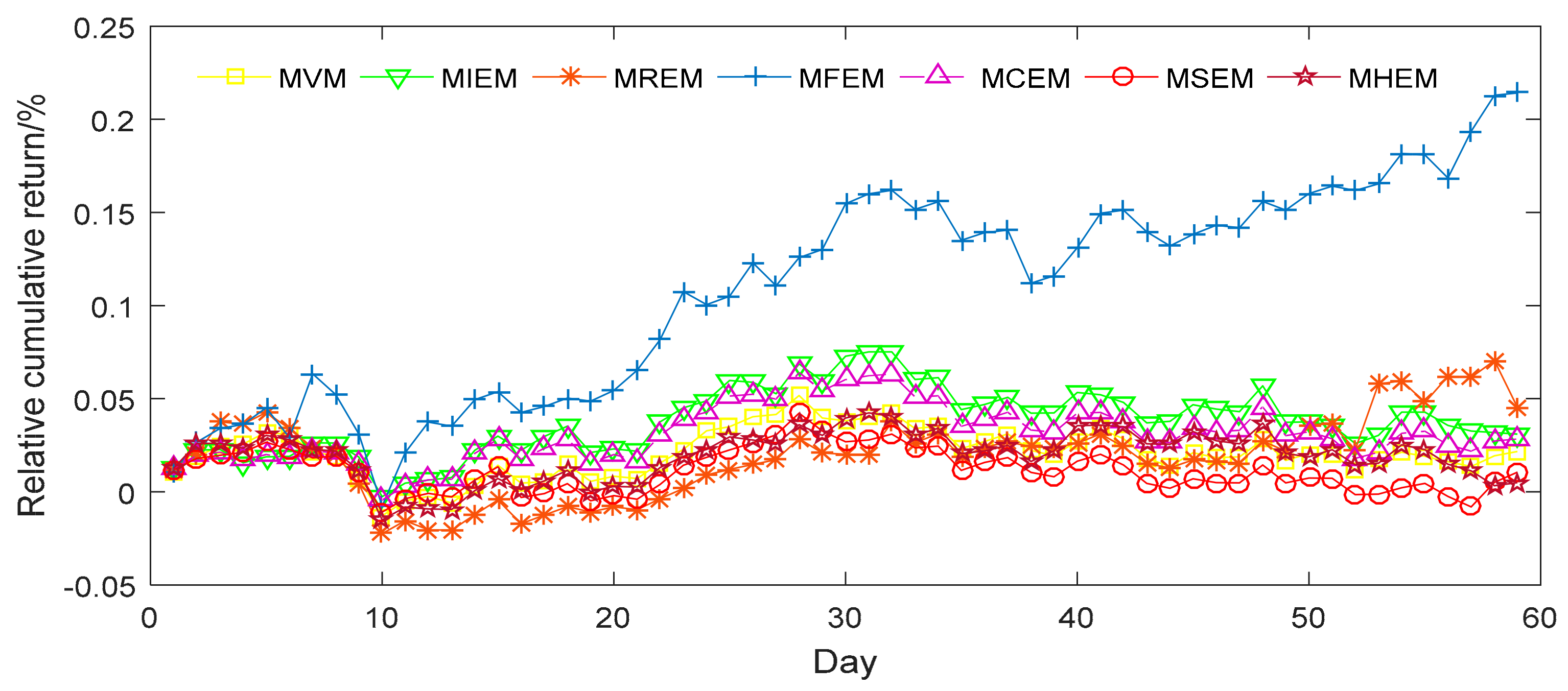
In order to appraise the investment performance of the seven different portfolio models, we can further predict the daily returns (DR) and relative cumulative returns (RCR) of each model. The price data of the corresponding stocks is taken from the period between 3 January 2017 and 1 April 2017. First, we can get the return of each stock of the period in the market. Then we assume that we have the seven portfolios based on the proportion obtained in Table 5. Therefore, we can calculate the returns and relative cumulative returns during the time. The results are shown in Figure 1 and Figure 2.
It is apparent from Figure 1 and Figure 2 that MFEM has both greater volatility in its DR and better general performance in its RCR than the alternative models. The DR and RCR of the other six models, meanwhile, are similar to one another. Furthermore, we evaluate means of DR and RCR for seven different models and display them in Table 6. MFEM clearly possesses the highest mean for RCR among the seven models. This result corroborates the above observation that MFEM has a higher degree of diversification. MCEM and MIEM have similar means, but perform slightly better than MVM, MREM, MSEM and MHEM. MHEM has the lowest means for DR and MSEM has the lowest means for RCR.
4.2.2. Empirical Analysis from American Sample Data
As was the case with the Chinese Shenzhen Stock Exchange, we selected nine listed stocks from nine different industries in the New York Stock Exchange of America. The stocks are shown in Table 7. The original data obtained from Yahoo Finance is composed of weekly data samples covering the period from 1 January 2011 to 1 January 2016, from which the weekly yields, highest possible yields and lowest possible yields can be calculated. Using Equations (1)–(6), we calculated the value of generalized entropy of the sample stocks. The results are shown in Table 8.
The covariance matrix for the nine stocks is calculated as follows:
According to the historical data in Table 7, when c is chosen as 0.0009, we can optimize the seven different portfolio models described in Section 4.1 and obtain their optimal investment proportions. The distinct results are presented in Table 9.
In Table 9, we can observe that, for MREM, the highest value in its optimal investment proportions exceeds 0.45. On the other hand, the highest value of optimal investment proportions is less than 0.45 in other models. This result shows that the degrees of diversification of MVM, MIEM, MFEM, MCEM and MSEM are more appropriate than that of MREM.
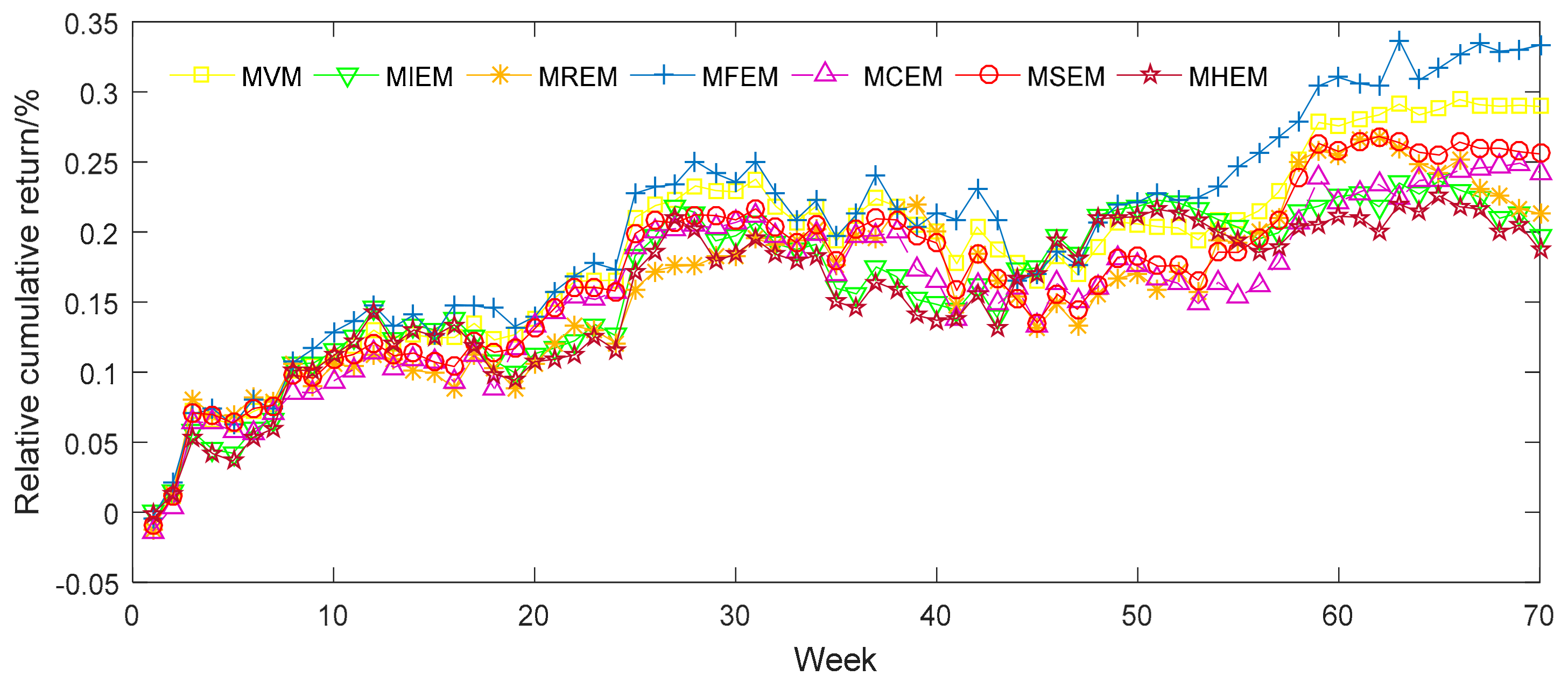
In order to appraise the investment performance of the seven different portfolio models, we can further predict the daily returns (DR) and relative cumulative returns (RCR) of each model. The weekly price data of the corresponding stocks was taken from the period between 1 January 2016 and 1 May 2017. The results are shown in Figure 3 and Figure 4.
Figure 3 and Figure 4 show that MFEM has better general performance in its RCR than the alternative models. The DR of the seven models, meanwhile, are similar to one another. For further analysis, we evaluate the means of DR and RCR for the seven different models and display them in Table 10. MFEM clearly possesses the highest mean for both DR and RCR among the seven models. This result corroborates the above observation that MFEM has a higher degree of diversification than some alternatives. MVM and MSEM have similar means, but perform slightly better than MIEM, MREM, MCEM and MHEM. MHEM has the lowest means for both DR and RCR.
Both of our empirical examples show that the highest value of optimal investment proportions is less than 0.45 in MFEM. In other words, MFEM has a higher degree of diversification than some worse-performing alternatives, and we think that the degree of diversification of MFEM is more appropriate. From our investment performance results, we see that MFEM has better general performance in terms of RCR than its alternatives in both empirical examples. In fact, the empirical results show MFEM clearly possesses the highest mean for both DR and RCR among the seven models.
5. Conclusions
Considering the fact that Entropy is widely used in portfolio selection as a risk measure, this paper systematically investigates the properties of risk measures of generalized entropy in financial field. These risk measures include Information Entropy, Cumulative Residual Entropy, Fuzzy Entropy, Credibility Entropy, Sine Entropy and Hybrid Entropy. Their properties include Monotonicity, Translation Invariance, Sub-additivity, Positive Homogeneity, Consistency, and Convexity. We find that no risk measure satisfies all six properties (and no risk measure satisfies monotonicity or translation invariance). Fuzzy Entropy, Credibility Entropy, and Sine Entropy all exhibit the same properties: Sub-additivity, Positive Homogeneity, Consistency, and Convexity. Information Entropy and Hybrid Entropy both only exhibit the properties of Sub-additivity and Consistency. Finally, Cumulative Residual Entropy satisfies just Sub-additivity, Positive Homogeneity, and Convexity.
In order to observe the actual performance of generalized entropy in portfolio selection problems, we construct seven portfolio models based on different risk measures. The empirical results from the samples of China and America show that MFEM performs the best among the seven models with respect to both DR and RCR, with the highest means in both categories.
Future research work can present two interesting avenues. On one hand, we can make some comparisons between the seven different portfolio models under the constraints of transaction costs, liquidity, and so on, instead of only expected return and risk. On the other hand, we can examine the implications of MFEM’s comparatively high performance for portfolio selection problems.
Acknowledgments
This work is partially supported by the National Natural Science Foundation of China under Grant No. 71631005, and the humanities and Social Science Foundation of the Ministry of Education under Grant No. 16YJA630078 and No. 14YJA790075, and the Major program for social and science of Beijing Grant No. 15ZDA46, and the central university basic scientific research operating expenses special funds of University of International Business and Economics Grant No. 15JQ04.
Author Contributions
Rongxi Zhou conceived, designed and revised the paper. Xiao Liu performed the experiments and wrote the paper. Mei Yu and Kyle Huang completed the discussion and polished the paper. All authors have read and approved the final manuscript.
Conflicts of Interest
The authors declare no conflict of interest.
References
- Markowitz, H.M. Portfolio selection. J. Financ. 1952, 7, 77–91. [Google Scholar]
- Markowitz, H.M. Portfolio Selection: Efficient Diversification of Investment; John Wiley: New York, NY, USA, 1959. [Google Scholar]
- Philippatos, G.C.; Wilson, C.J. Entropy, market risk, and the selection of efficient portfolios. Appl. Econ. 1972, 4, 209–220. [Google Scholar] [CrossRef]
- Konno, H.; Yamazaki, H. Mean-absolute deviation portfolio optimization model and its application to Tokyo stock market. Manag. Sci. 1991, 37, 519–531. [Google Scholar] [CrossRef]
- Cai, X.Q.; Teo, K.L.; Yang, X.Q.; Zhou, X.Y. Portfolio optimization under a minimax rule. Manag. Sci. 2000, 46, 957–972. [Google Scholar] [CrossRef]
- Jorion, P. Measure the risk in value at risk. Financ. Anal. J. 1996, 52, 47–55. [Google Scholar] [CrossRef]
- Rockafellar, R.T.; Uryasev, S. Optimization of Conditional value at risk. J. Risk. 2000, 2, 21–41. [Google Scholar] [CrossRef]
- Acerbi, C.; Tasche, D. On the coherence of expected shortfall. J. Bank. Financ. 2002, 26, 1487–1503. [Google Scholar] [CrossRef]
- Zhou, R.X.; Cai, R.; Tong, G.Q. Applications of Entropy in Finance: A Review. Entropy 2013, 15, 4909–4931. [Google Scholar] [CrossRef]
- Philippatos, G.C.; Gressis, N. Conditions of equivalence among E-V, SSD, and E-H portfolio selection criteria: The case for uniform, normal and lognormal distributions. Manag. Sci. 1975, 21, 617–625. [Google Scholar] [CrossRef]
- Nawrocki, D.N.; Harding, W.H. State-value weighted entropy as a measure of investment risk. Appl. Econ. 1986, 18, 411–419. [Google Scholar] [CrossRef]
- Smimou, K.; Bector, C.R.; Jacoby, G. A subjective assessment of approximate probabilities with a portfolio application. Res. Int. Bus. Financ. 2007, 21, 134–160. [Google Scholar] [CrossRef]
- Huang, X.X. Mean-Entropy Models for Fuzzy Portfolio Selection. IEEE Trans. Fuzzy Syst. 2008, 16, 1096–1101. [Google Scholar] [CrossRef]
- Xu, J.P.; Zhou, X.; Wu, D.D. Portfolio selection using λ mean and hybrid entropy. Ann. Oper Res. 2011, 185, 213–229. [Google Scholar] [CrossRef]
- Usta, I.; Kantar, Y.M. Mean-Variance-Skewness-Entropy Measures: A Multi-Objective Approach for Portfolio Selection. Entropy 2011, 13, 117–133. [Google Scholar] [CrossRef]
- Zhang, W.G.; Liu, Y.J.; Xu, W.J. A possibilistic mean-semivariance- entropy model for multi-period portfolio selection with transaction costs. Eur. J. Oper. Res. 2012, 222, 341–349. [Google Scholar] [CrossRef]
- Zhou, R.X.; Wang, X.G.; Dong, X.F.; Zong, Z. Portfolio Selection Model with the Measures of Information Entropy-Incremental Entropy-Skewness. Adv. Inf. Sci. Serv. Sci. 2013, 5, 853–864. [Google Scholar]
- Zhang, W.G.; Liu, Y.J.; Xu, W.J. A new fuzzy programming approach for multi-period portfolio optimization with return demand and risk control. Fuzzy Set. Syst. 2014, 246, 107–126. [Google Scholar] [CrossRef]
- Yao, K. Sine entropy of uncertain set and its applications. Appl. Soft Comput. 2014, 22, 432–442. [Google Scholar] [CrossRef]
- Yu, J.R.; Lee, W.Y.; Chiou, W.J.P. Diversified portfolios with different entropy measures. Appl. Math. Comput. 2014, 241, 47–63. [Google Scholar] [CrossRef]
- Zhou, R.X.; Zhan, Y.; Cai, R.; Tong, G.Q. A Mean-Variance Hybrid-Entropy Model for Portfolio Selection with Fuzzy Returns. Entropy 2015, 17, 3319–3331. [Google Scholar] [CrossRef]
- Gao, J.W.; Liu, H.C. A Risk-Free Protection Index Model for Portfolio Selection with Entropy Constraint under an Uncertainty Framework. Entropy 2017, 19, 1–12. [Google Scholar] [CrossRef]
- Ramsay, C.M. Loading gross premiums for risk without using utility theory. Trans. Soc. Actuar. 1993, 45, 305–349. [Google Scholar]
- Artzner, P.; Delbaen, F.; Eber, J.M.; Heath, D. Coherent Measures of Risk. Math. Financ. 1999, 9, 203–228. [Google Scholar] [CrossRef]
- Follmer, H.; Schied, A. Convex measures of risk and trading constraints. Financ. Stoch. 2002, 6, 429–447. [Google Scholar] [CrossRef]
- Bali, T.G.; Cakici, N.; Fousseni, C.Y. A Generalized Measure of Riskiness. Manag. Sci. 2011, 57, 1406–1423. [Google Scholar] [CrossRef]
- Zheng, C.L.; Chen, Y. Coherent risk measure based on relative entropy. Appl. Math. Inform. Sci. 2012, 6, 233–238. [Google Scholar]
- Gaivoronski, A.; Pflug, G. Value at Risk in Portfolio Optimization; Properties and Computational Approach; Technical Report; University of Vienna: Wien, Austria, 2001. [Google Scholar]
- Shannon, C.E. A mathematical theory of communication. Bell Syst. Tech. J. 1948, 27, 379–423. [Google Scholar] [CrossRef]
- Cao, X.H. Information Theory and Coding; Tsinghua University Press: Beijing, China, 2009. [Google Scholar]
- Rao, M.; Chen, Y.; Vemuri, B.; Fei, W. Cumulative residual entropy: A new measure of information. IEEE Trans. Inf. Theory 2004, 50, 1220–1228. [Google Scholar] [CrossRef]
- Liu, B.D. Uncertain logic for modeling human language. J. Uncertain Syst. 2011, 5, 3–20. [Google Scholar]
- Liu, B.D. A Survey of Entropy of Fuzzy Variables. J. Uncertain Syst. 2007, 1, 4–13. [Google Scholar]
- Liu, B.D. Membership functions and operational law of uncertain sets. Fuzzy Optim. Decis. Mak. 2012, 11, 387–410. [Google Scholar] [CrossRef]
- Yao, K.; Ke, H. Entropy operator for membership function of uncertain set. Appl. Math. Comput. 2014, 242, 898–906. [Google Scholar] [CrossRef]
- Li, P.K.; Liu, B.D. Entropy of credibility distributions for fuzzy variables. IEEE Trans. Fuzzy Syst. 2008, 16, 123–129. [Google Scholar]
- Yao, K. Sine entropy of uncertain variables. Int. J. Uncertain. 2013, 21, 743–753. [Google Scholar] [CrossRef]
- Shang, X.G.; Jiang, W.S. Rationality Analysis and Promotion of De Luca-Termini Hybrid Entropy. J. East China Univ. Sci. Technol. 1996, 23, 590–595. [Google Scholar]
Figure 1.
The daily returns of samples from seven different portfolio models.
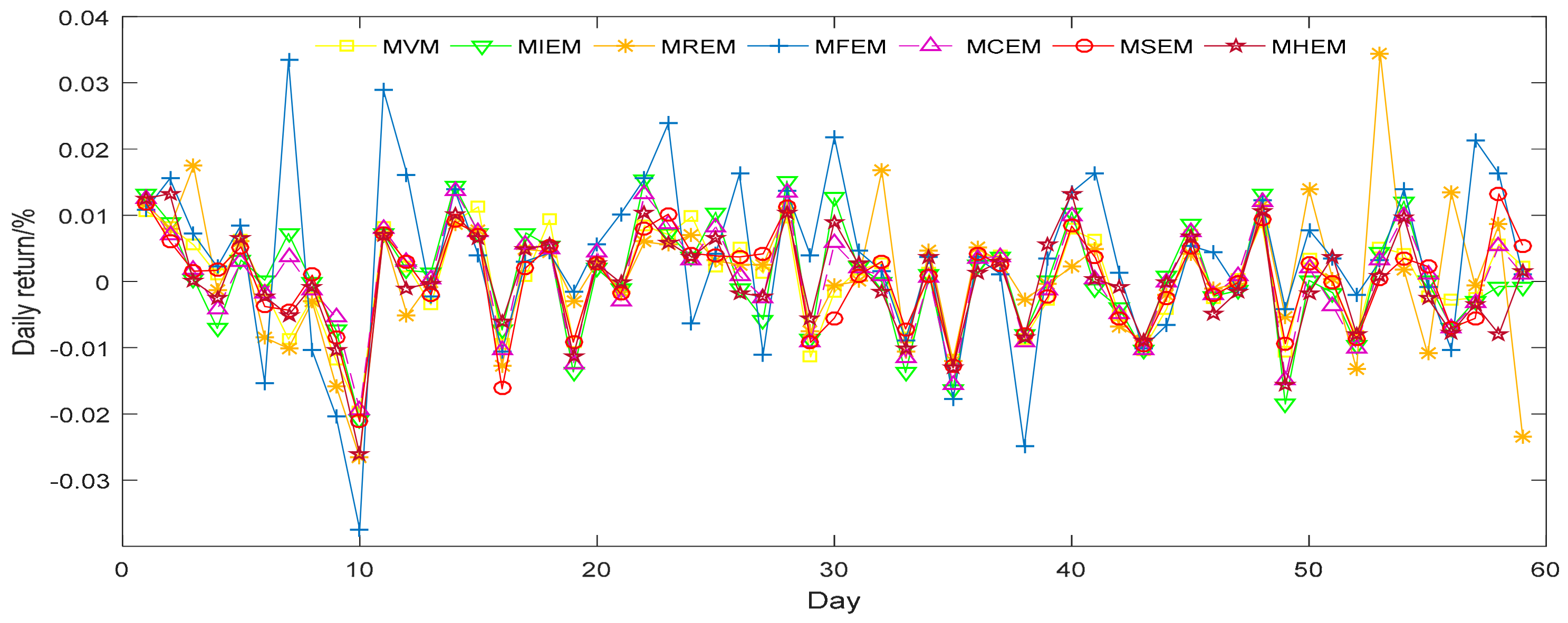
Figure 2.
The relative cumulative returns of samples from seven different portfolio models.

Figure 3.
The daily returns of samples from seven different portfolio models.
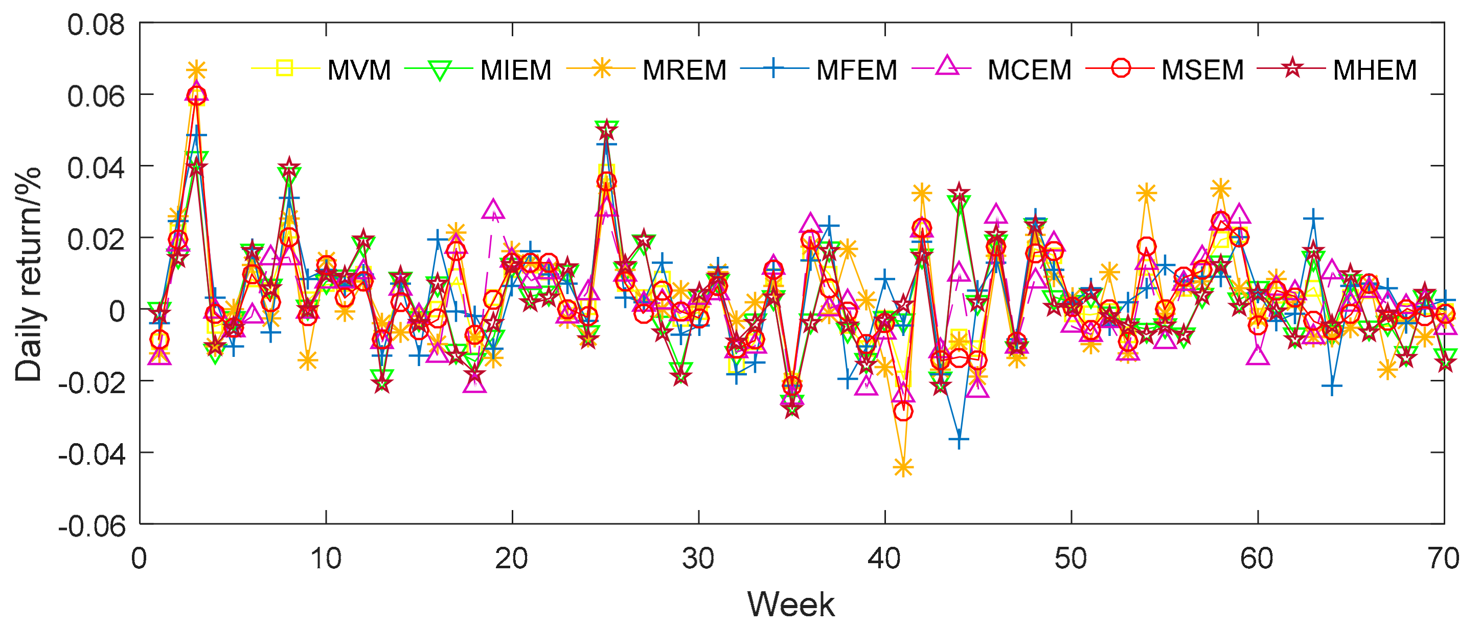
Figure 4.
The relative cumulative returns of samples from seven different portfolio models.


Table 1.
The properties of risk measures of generalized entropy.
| Information Entropy | Cumulative Residual Entropy | Fuzzy Entropy | Credibility Entropy | Sine Entropy | Hybrid Entropy | |
|---|---|---|---|---|---|---|
| Monotonicity | × | × | × | × | × | × |
| Translation Invariance | × | × | × | × | × | × |
| Sub-additivity | √ | √ | √ * | √ * | √ * | √ * |
| Positive Homogeneity | × | √ | √ | √ | √ | × |
| Consistency | √ | × | √ | √ | √ | √ |
| Convexity | × | √ | √ * | √ * | √ * | × |
Remark: * represents that the two fuzzy variables are independent.
Table 2.
The seven models and corresponding risk measure.
| Model Name | Risk Measure |
|---|---|
| Mean and Variance Model (MVM) | |
| Mean Information Entropy Model (MIEM) | |
| Mean Residual Entropy Model (MREM) | |
| Mean Fuzzy Entropy Model (MFEM) | |
| Mean Credibility Entropy Model (MCEM) | |
| Mean Sine Entropy Model (MSEM) | |
| Mean Hybrid Entropy Model (MHEM) |
Note: here ξ is a variable, which represents a random variable in the first three models and a fuzzy variable in other models.
Table 3.
Ten Chinese sample stocks collected from ten industries.
| Stock Code | Industry | Company Name |
|---|---|---|
| 002116 | Scientific research and technology service | China Haisum Engineering Co Ltd |
| 000966 | Utilities | Guodian Changyuan Electric Power Co Ltd |
| 000005 | Water resources, environment and public facilities management | Shenzhen Fountain Corporation |
| 000937 | Mining | Jizhong Energy Resources Co Ltd |
| 000882 | Leasing and business services | Beijing Hualian Department Store Co Ltd |
| 000776 | Finance | GF Securities Co Ltd |
| 000010 | Construction | Beijing Shenhuaxin Co Ltd |
| 000022 | Transportation, warehousing and postal services | Shenzhen Chiwan Wharf Holdings Co Ltd |
| 000592 | Agriculture, forestry, livestock farming, fishery | Zhongfu Straits (Pingtan) Development Co Ltd |
| 000837 | Manufacturing | Qinchuan Machinery Development Co Ltd of Shaanxi |
Table 4.
Expected values, Variance and generalized entropy for ten stocks.
| Stock Code | Expected Value | Variance | Information Entropy | Cumulative Residual Entropy |
| 002116 | 0.000358 | 0.000684 | 0.522250 | 0.014387 |
| 000966 | 0.000106 | 0.000411 | 0.522197 | 0.010422 |
| 000005 | 0.000583 | 0.000771 | 0.495046 | 0.018321 |
| 000937 | 0.002914 | 0.000879 | 0.541494 | 0.020575 |
| 000882 | 0.001688 | 0.000690 | 0.517706 | 0.014476 |
| 000776 | 0.001089 | 0.000443 | 0.486794 | 0.013178 |
| 000010 | 0.001764 | 0.000831 | 0.536057 | 0.018320 |
| 000022 | 0.001292 | 0.000717 | 0.555807 | 0.015292 |
| 000592 | –0.001478 | 0.000942 | 0.529302 | 0.019134 |
| 000837 | 0.000007 | 0.000784 | 0.524759 | 0.020385 |
| Stock Code | Fuzzy Entropy | Credibility Entropy | Sine Entropy | Hybrid Entropy |
| 002116 | 0.917527 | 0.017518 | 0.022316 | 0.768799 |
| 000966 | 0.909969 | 0.012838 | 0.016354 | 0.798535 |
| 000005 | 0.925415 | 0.018119 | 0.023081 | 0.752247 |
| 000937 | 0.921937 | 0.023726 | 0.030225 | 0.825716 |
| 000882 | 0.923970 | 0.020318 | 0.025883 | 0.767248 |
| 000776 | 0.907789 | 0.014732 | 0.018767 | 0.752970 |
| 000010 | 0.923278 | 0.017534 | 0.022336 | 0.812668 |
| 000022 | 0.894561 | 0.020841 | 0.026549 | 0.829238 |
| 000592 | 0.922229 | 0.017690 | 0.022535 | 0.794126 |
| 000837 | 0.832758 | 0.016749 | 0.021337 | 0.802894 |
Table 5.
The proportion of sample stocks in different portfolio models.
| Stock Code | MVM | MIEM | MREM | MFEM | MCEM | MSEM | MHEM |
|---|---|---|---|---|---|---|---|
| 002116 | 0.0662 | 0.0189 | 0.450 | 0.0149 | 0.0181 | 0.0106 | 0.0077 |
| 000966 | 0.4994 | 0.0341 | 0.4056 | 0.1194 | 0.2561 | 0.6104 | 0.0508 |
| 000005 | 0.0349 | 0.0911 | 0.0011 | 0.0605 | 0.0043 | 0.0110 | 0.3407 |
| 000937 | 0.1124 | 0.0005 | 0.0006 | 0.0009 | 0.0015 | 0.0016 | 0.0011 |
| 000882 | 0.0518 | 0.0621 | 0.0007 | 0.0167 | 0.0017 | 0.0008 | 0.0547 |
| 000776 | 0.1368 | 0.7124 | 0.1315 | 0.0767 | 0.5738 | 0.2742 | 0.4900 |
| 000010 | 0.0380 | 0.0089 | 0.0013 | 0.0258 | 0.0754 | 0.0241 | 0.0146 |
| 000022 | 0.0392 | 0.0016 | 0.0050 | 0.1899 | 0.0037 | 0.0013 | 0.0188 |
| 000592 | 0.0202 | 0.0125 | 0.0029 | 0.1069 | 0.0089 | 0.0516 | 0.0132 |
| 000837 | 0.0011 | 0.0579 | 0.0005 | 0.3883 | 0.0565 | 0.0144 | 0.0084 |
Table 6.
The means of daily returns and relative cumulative returns for seven different portfolio models.
Table 6.
The means of daily returns and relative cumulative returns for seven different portfolio models.
| MVM | MIEM | MREM | MFEM | MCEM | MSEM | MHEM | |
|---|---|---|---|---|---|---|---|
| DR | 0.00039 | 0.00055 | 0.00080 | 0.00338 | 0.00050 | 0.00020 | 0.00011 |
| RCR | 0.02074 | 0.03744 | 0.01912 | 0.10800 | 0.03087 | 0.01128 | 0.01937 |
Table 7.
Nine American sample stocks collected from nine industries.
| Stock Code | Industry | Company Name |
|---|---|---|
| XOM | Basic Materials | Exxon Mobil Corporation |
| NEE | Utilities | NextEra Energy, Inc. |
| PG | Consumer Goods | The Procter & Gamble Company |
| JNJ | Healthcare | Johnson & Johnson |
| T | Technology | AT&T Inc. |
| BCH | Financial | Banco de Chile |
| WMT | Services | Wal-Mart Stores, Inc. |
| GE | Industrial Goods | General Electric Company |
| HRG | Conglomerates | HRG Group, Inc. |
Table 8.
Expected values, Variance and generalized entropy for ten stocks.
| Stock Code | Expected Value | Variance | Information Entropy | Cumulative Residual Entropy |
| XOM | 0.000684 | 0.000667 | 0.579663 | 0.009051 |
| NEE | 0.002050 | 0.000476 | 0.617725 | 0.007630 |
| PG | 0.001078 | 0.000382 | 0.597884 | 0.006739 |
| JNJ | 0.001719 | 0.000333 | 0.595278 | 0.006417 |
| T | 0.000886 | 0.000472 | 0.582108 | 0.007338 |
| BCH | –0.001058 | 0.000906 | 0.547013 | 0.009808 |
| WMT | 0.001595 | 0.000533 | 0.622009 | 0.008027 |
| GE | 0.001872 | 0.000858 | 0.546699 | 0.010659 |
| HRG | 0.001702 | 0.001756 | 0.625417 | 0.014955 |
| Stock Code | Fuzzy Entropy | Credibility Entropy | Sine Entropy | Hybrid Entropy |
| XOM | 0.954630 | 0.018010 | 0.022943 | 0.856335 |
| NEE | 0.935999 | 0.016779 | 0.021374 | 0.891082 |
| PG | 0.929912 | 0.014469 | 0.018432 | 0.876359 |
| JNJ | 0.946126 | 0.014319 | 0.018241 | 0.877410 |
| T | 0.963329 | 0.016518 | 0.021042 | 0.862157 |
| BCH | 0.939306 | 0.022284 | 0.028387 | 0.829200 |
| WMT | 0.960407 | 0.015609 | 0.019883 | 0.894488 |
| GE | 0.909638 | 0.020336 | 0.025906 | 0.838212 |
| HRG | 0.943969 | 0.036577 | 0.046594 | 0.890792 |
Table 9.
The proportion of sample stocks in different portfolio models.
| Stock Code | MVM | MIEM | MREM | MFEM | MCEM | MSEM | MHEM |
|---|---|---|---|---|---|---|---|
| XOM | 0.0081 | 0.0492 | 0.0007 | 0.0011 | 0.0019 | 0.0022 | 0.0679 |
| NEE | 0.1468 | 0.0010 | 0.0033 | 0.4415 | 0.0263 | 0.2012 | 0.0010 |
| PG | 0.2469 | 0.0902 | 0.7990 | 0.0816 | 0.2990 | 0.3991 | 0.0834 |
| JNJ | 0.2063 | 0.0839 | 0.1713 | 0.0451 | 0.1509 | 0.1537 | 0.0150 |
| T | 0.0938 | 0.1074 | 0.0185 | 0.1128 | 0.1000 | 0.0826 | 0.0737 |
| BCH | 0.1289 | 0.2412 | 0.0012 | 0.2363 | 0.0001 | 0.0002 | 0.2515 |
| WMT | 0.1652 | 0.0014 | 0.0037 | 0.0159 | 0.4201 | 0.1598 | 0.0278 |
| GE | 0.0009 | 0.4248 | 0.0012 | 0.0423 | 0.0011 | 0.0003 | 0.4671 |
| HRG | 0.0031 | 0.0009 | 0.0011 | 0.0234 | 0.0006 | 0.0009 | 0.0126 |
Table 10.
The means of daily returns and relative cumulative returns for seven different portfolio models.
Table 10.
The means of daily returns and relative cumulative returns for seven different portfolio models.
| MVM | MIEM | MREM | MFEM | MCEM | MSEM | MHEM | |
|---|---|---|---|---|---|---|---|
| DR | 0.00372 | 0.00268 | 0.00289 | 0.00422 | 0.00321 | 0.00334 | 0.00256 |
| RCR | 0.18683 | 0.16366 | 0.16107 | 0.20296 | 0.15893 | 0.17101 | 0.15561 |
© 2017 by the authors. Licensee MDPI, Basel, Switzerland. This article is an open access article distributed under the terms and conditions of the Creative Commons Attribution (CC BY) license (http://creativecommons.org/licenses/by/4.0/).
Share and Cite
MDPI and ACS Style
Zhou, R.; Liu, X.; Yu, M.; Huang, K. Properties of Risk Measures of Generalized Entropy in Portfolio Selection. Entropy 2017, 19, 657. https://doi.org/10.3390/e19120657
AMA Style
Zhou R, Liu X, Yu M, Huang K. Properties of Risk Measures of Generalized Entropy in Portfolio Selection. Entropy. 2017; 19(12):657. https://doi.org/10.3390/e19120657
Chicago/Turabian StyleZhou, Rongxi, Xiao Liu, Mei Yu, and Kyle Huang. 2017. "Properties of Risk Measures of Generalized Entropy in Portfolio Selection" Entropy 19, no. 12: 657. https://doi.org/10.3390/e19120657
Note that from the first issue of 2016, this journal uses article numbers instead of page numbers. See further details here.