Capturing Causality for Fault Diagnosis Based on Multi-Valued Alarm Series Using Transfer Entropy


1
Shandong Electric Power Research Institute for State Grid Corporation of China, Jinan 250003, China
2
College of Urban Rail Transit and Logistics, Beijing Union University, Beijing 100101, China
3
Tsinghua Laboratory for Information Science and Technology and Department of Automation, Tsinghua University, Beijing 100084, China
*
Author to whom correspondence should be addressed.
Entropy 2017, 19(12), 663; https://doi.org/10.3390/e19120663
Submission received: 1 November 2017
/
Revised: 24 November 2017
/
Accepted: 29 November 2017
/
Published: 4 December 2017
(This article belongs to the Special Issue Entropy and Complexity of Data)
Abstract
:Transfer entropy (TE) is a model-free approach based on information theory to capture causality between variables, which has been used for the modeling and monitoring of, and fault diagnosis in, complex industrial processes. It is able to detect the causality between variables without assuming any underlying model, but it is computationally burdensome. To overcome this limitation, a hybrid method of TE and the modified conditional mutual information (CMI) approach is proposed by using generated multi-valued alarm series. In order to obtain a process topology, TE can generate a causal map of all sub-processes and modified CMI can be used to distinguish the direct connectivity from the above-mentioned causal map by using multi-valued alarm series. The effectiveness and accuracy rate of the proposed method are validated by simulated and real industrial cases (the Tennessee-Eastman process) to capture process topology by using multi-valued alarm series.
1. Introduction
With the development of science and technology, modern industrial systems have become increasingly complex, which brings new challenges to industrial process system design, industrial process control, and industrial safety. In these conditions, the large number of sensors used leads to an abundance of complex observational data that are difficult to understand, and the mechanism for complex interaction between devices is not fully understood. Models play a vital role in understanding these matters, but it is quite difficult to obtain a precise model. In the control and automation community, an underlying model can be obtained by analyzing connectivity and causality, which also have a number of potential applications in the analysis and design of, and fault diagnosis in, large complex industrial processes [1]. In other words, a process topology can be used for risk assessment, root cause analysis, and consequential alarm series identification by using the information of fault propagation [2]. Moreover, capturing the causality between variables when only time series are given is of very general interest in many fields of science, especially when an underlying model is poorly understood. Considering the climate system, capturing causality reveals a rich internal structure in complex climate networks [3,4]. Also, the discovery of causal relationships in economic data and the inference of functional brain connectivity in neurosciences are of great importance [2,5,6,7,8].
From the 1970s onward, a signed directed graph (SDG) has been used to describe a system as a graphical representation of causal relations amongst variables. It can be used to find fault propagation paths and to explain the causes for a fault [9]. The modeling of SDGs needs to collect process knowledge; specifically, a piping and instrumentation diagram (P&ID) and equations [10]. The establishment of the above method basically depends on human effort. Obviously, such an SDG modeling method is not suitable for modern complex industrial processes. Later, a statistical approach was proposed, and it can be used to detect correlation and time delays, and exclude other influences between industrial processes when only some time series of measurements are given. Various data-based approaches, which mainly include the cross-correlation function (CCF), the Bayesian network, Granger causality, and partial directed coherence (PDC), are popular in many fields of science. The CCF can be used to estimate the time delay between process measurements and capture the connectivity between process variables, but cannot detect the causal relations between them [11]. The Bayesian network, a conditional independence method, provides a graph with probabilities [12]. However, its major limitation is that the physical explanation of probabilities is not straightforward, which is unacceptable by engineers sometimes [1]. Granger causality, a dynamic approach, requires a linear regression model [8,13]. In other words, this method describes a linear causality relationship and needs to assume a linear relation between the process variables. PDC is a standardized method which detects direct causal relationships between two variables in multiple variables [14]. These causal analysis methods not only provide a reference for engineers to understand industrial processes’ underlying models, but also make it possible for us to understand extreme weather phenomena (such as the El Niño phenomenon and the Indian monsoon) and promote research in economics and neurosciences [2,3,4,5,6,7,8].
The above-mentioned methods can accurately detect a causal relationship between process variables, but they are only suitable for linear models. In practice, if the process has strong nonlinearity and cannot be identified as a linear model, then a more general approach should be used. Transfer entropy (TE) is a model-free method to capture causality in complex industrial processes. It is able to detect causality between couples of variables, regardless of any underlying models. Therefore, it is of general interest in many fields of science, especially when only time series data are given and the underlying model is difficult to understand. In modern industrial processes, TE has successfully detected causality between variables based on processes’ time series [15]. However, it is a bivariate analysis method, which cannot detect direct causality that excludes indirect influences or common drivers. A modified TE can be used to solve some specific problems. For example, the direct transfer entropy (DTE) concept is proposed to detect whether there is a direct information flow pathway from one variable to another [16]. Compared to TE, the probability density function (PDF) of DTE is more complex; transfer 0-entropy (T0E) was proposed for a causality analysis on the basis of the definitions of 0-entropy and 0-information without assuming a probability space [17].
Most of the above modified TE methods are computationally burdensome. To solve this problem, Staniek et al. [18] proposed the symbolic transfer entropy. However, the physical meaning of the symbols is not straightforward. Then, Yu et al. [19] proposed transfer entropy to detect causality between process variables based on alarm data, which can replace process data with binary alarm series. Its main contribution is a new application of TE that uses binary alarm data for causality detection, while a lot of information contained in the process data is lost. Thus, this method may lead to erroneous conclusions.
In this work, the main contribution is to propose a hybrid method based on TE and modified conditional mutual information (CMI) with a lower computational cost, which detects direct causality between variables by using the modified alarm series. TE is used to capture the causality between variables. CMI is used to distinguish direct connectivity from the causality map detected by TE.
2. Alarm Series and Its Extended Form
This section will introduce binary alarm series and multi-valued alarm series. In addition, we use an example to exemplify the difference between binary alarm series and multi-valued alarm series.
2.1. Binary Alarm Series
In modern industrial alarm systems, alarm variables can be generated based on continuous variables. However, this is not the case for switch variables (e.g., ON/OFF) and status variables [19]. In this work, taking the alarm series that are generated by comparing the corresponding thresholds for continuous variables as an example, we introduce the proposed methods.
In alarm systems, x is the binary alarm sequence generated by setting the alarm threshold for a process variable p. The binary alarm series x usually has two states [19,20,21]. The first one is 0 when the process variable p is in the normal state; otherwise, x takes the value 1. Given the variable p, x is generated by
where indicates the upper limit of the normal states as threshold. In this formula, the binary alarm series x only indicates whether the process variable p remains in the normal state, while most of the other information (such as error, alarm, and warning) is ignored. So, the detection of causality based on the above-mentioned alarm series x may lead to the production of erroneous conclusions.
For example, there are two uncorrelated random time series A and B, as shown in Figure 1. Based on those time series, the CCF value that is calculated from B to A by using process data is 0.15080 and the corresponding lag is 245. The window size of the CCF is the length of the time series (the length of the time series is 1000).
When we choose the upper limit (H) as 2, the binary alarm series xi configured by time series A and B are shown in Figure 2. It is easy to find that the time series that are completely different from each other become similar to the original time series. The max CCF value that is calculated from B to A by using the binary alarm series is 0.24580 and the corresponding lag is −71. It is obvious that the conclusion based on the binary alarm series xi is incorrect.
2.2. Multi-Valued Alarm Series
As we know, every alarm event corresponds to a certain state in distributed control systems (DCSs). The alarm types are usually composed of the high error (HHH), high alarm (HH), high warning (HI), low warning (LO), low alarm (LL), and low error (LLL) types [21]. For example, measured value monitoring (MEAS_MON), a function block (FB) of SIMATIC PCS7, has four types of alarms, namely, high alarm (HH), high warning (HI), low warning (LO), and low alarm (LL), as shown in Figure 3.
To solve the problem mentioned in Section 2.1, we propose a multi-valued alarm series that embeds the information in different alarm types configured on the same process variable, and it is actually a combination of multiple binary alarm sequences (such as HH, HI, LO, and LL). The proposed multi-valued alarm series reduces the information loss in an alarm series generated from the corresponding process sequence and lessens the chance of error. Moreover, it does not bring extra computational cost. So, it is more suitable to detect causality between variables using the proposed multi-valued alarm series that to detect it using a binary alarm series.
If we have already obtained several binary alarm series of a variable p, such as HH, HI, LO, and LL, then the multi-valued alarm series x is generated by
where HH, HI, LO, and LL denote different alarm states of the variable p; and “normal” denotes that p is in the normal state.
As shown in Figure 4a,b, the HH, HI, LO, and LL alarm series are generated by the continuous variables A and B, respectively. Then, the multi-valued alarm series obtained by Equation (2) are shown in Figure 4c.
All of the CCFs based on the above-mentioned three different series are shown in Table 1. According to the obtained results, the detection of causality using multi-valued alarm series is closer to that using the original process data than the detection of causality using binary alarm series.
In modern industrial systems, not only does a process variable have different alarm states, such as HI, LO, HH, and LL, and even HHH and LLL, but also the equipment and the industrial system have many different abnormal states. For the equipment, the common intelligent alarm states of a motor include voltage anomalies, winding ground, winding short circuit, winding open circuit, and phase loss; for the industrial system, common faults include overload operation and mixer failure. The above-mentioned abnormal states, including variable alarms, device intelligence alarms, or system failures, can be denoted as Si (i = 1, 2, 3, …, n), which are the different states of a multi-valued alarm series. Hence, the causality between variables or equipment or systems via multi-valued alarm series can be detected.
3. Transfer Entropy and Mutual Information
This section introduces TE, mutual information (MI), and CMI. In addition, we will introduce how to detect direct causality between variables based on these methods.
3.1. Transfer Entropy
Transfer entropy was proposed by Schreiber in 2000. It provides an information-theoretic method to detect causality by measuring the reduction of uncertainty [22]. According to information theory, the TE formula from variable X = [x1, x2, x3, …, xt, …, xn]’ to Y = [y1, y2, y3, …, yt, …, yn]’ is defined as
where xt and yt denote the values of the variables X and Y, respectively, at time t; k and l denote the orders of the cause variable and effect variable, respectively; xt and its l-length past are defined as ; yt and its past are defined as ; τ is the sampling period; h denotes the prediction horizon; ω is the random vector ; and f denotes the complete or conditional PDF. In this TE method, the PDF can be estimated by kernel methods or a histogram [23], which are nonparametric approaches, to fit any shape of the distributions.
According to TE, if there is causality from variables X to Y, then it is helpful to predict Y via the historical data of X. In other words, the information of Y can be obtained from the historical values of Y and X. Then, and the TE should be positive. Otherwise, it should be close to zero.
In (3), Y and X are two continuous time series. So, Equation (3) is not suitable for discrete time series. Then, a discrete transfer entropy (TEdisc) from X toY, for discrete time series, is estimated as follows:
where the meanings of the symbols in this form is similar to those in (3). Variables and denote the discrete time series, , ; h denotes the prediction horizon; p denotes the complete or conditional PDF; τ is the sampling period; and k and l denote the orders of the cause variable and the effect variable, respectively.
3.2. Conditional Mutual Information
This section introduces MI and CMI, which are information-theoretic methods [24].
3.2.1. Mutual Information
MI is a method that can detect the degree of independence between two random time series. The MI formula between variables X = [x1, x2, x3, …, xn]’ and Y = [y1, y2, y3, …, yn]’ is defined as [25]
where xt and yt denote the value of variables X and Y, respectively, at time t; denotes the joint PDFs of X and Y; and and are the marginal PDFs of X and Y, respectively. The summation is on the feasible space of x and y and will be omitted hereinafter for brevity.
In order to estimate the MI between Y and the historical data of X, the modified MI method is defined as
It can be seen that the TE formula in (4) is similar to (6). Figure 5 shows the tendency of the TEs and modified MIs based on four simulation variables (A, B, C, and D that will be analyzed later) within the prediction range h = 1 to 50 (according to Yu et al. [19], k = l = 1, τ = 1).
It is shown that the TE and the modified MI methods obtain a maximum value at a similar h. Therefore, the prediction horizon h can be determined via the modified MI.
3.2.2. Conditional Mutual Information
CMI is the expected value of the MI of two random variables given a third one. The CMI formula between variables X = [x1, x2, x3, …, xn]’ and Y = [y1, y2, y3 , …, yn]’ conditioned on Z = [z1, z2, z3, …, zn]’ is defined as [25]
where xt, yt, and zt denote the value of the variables X, Y, and Z respectively at time t; denotes the joint PDF of X, Y, and Z; and denotes the joint PDF of X and Y given Z. and are the PDF of X given Z and the PDF of Y given Z, respectively.
If Y = yt+h, , and , the CMI formula in Equation (7) is expressed as Equation (8). By doing so, the CMI is equivalent to the TE formula in Equation (3). Therefore, the TE formula is a special case of Equation (7) [26].
The above-mentioned DTE of the variables X and Y given variable Z is also a special case of CMI, and is formulated as [16]
where the meanings of the symbols in this formula are similar to those in Equation (3). It is obvious that Equation (9) is more complex than (7). Therefore, if we have already obtained causality between variables, CMI is friendlier than DTE on computational cost, while distinguishing between direct causality from the causality map detected by TE between two variables, given the third one.
In this work, in order to distinguish direct from indirect causality between two variables conditioned on a third, modified CMI is defined as
and can be simplified as
where h1 denotes the prediction horizon from Y to X; and h2 denotes the prediction horizon from Z to X.
4. Detection of Direct Causality via Multi-Valued Alarm Series
This section will introduce the detection of causality between process variables via discrete TE by using multi-valued alarm series. In addition, modified CMI is used to distinguish a direct from an indirect causality.
4.1. Detection of Causality via TE
If we have already obtained several binary alarm series of variables, such as HH, HI, LO, and LL, then the multi-valued alarm series can be obtained by Equation (2).
The next step is to estimate the TEs between all sub-processes by using the multi-valued alarm series generated by Equation (2). The four parameters need to be determined beforehand in Equation (4). Here, according to Yu et al. [19], we select k = l = 1, τ = 1, and the prediction horizon h is determined by the modified MI mentioned above.
Then, the TEs are shown in Figure 6. An underlying model is A→B→D. However, the TE method, a bivariate analysis, can capture a significant causality between A and D, which is an indirect causality in a multivariate analysis including B. It is found that those causalities may include an indirect one.
TE is a bivariate analysis. Thus, from the causality map based on TE, it is easy to get a wrong conclusion that the link A→D is a direct coupling. So, we need other effective ways to analyze this problem.
4.2. Detection of Direct Causality via CMI
To overcome the limitation of TE in Figure 6, modified CMI is embedded into our method to distinguish direct connectivity from the causality map detected by TE [27]. In Figure 6, there are two links from A to D: (1) the link directly from A to D (A→D); and (2) the link from A to D via B (A→B→D). So, the link from A to D may be a direct or an indirect coupling. When the underlying model is poorly understood, the above-mentioned TE is unable to distinguish whether the causality between variables A and D is along a direct link or through variable B. By estimating the modified CMI from A to D given B, we can determine the connectivity between A and D. Then, combining the above CMIs and the TEs in Section 4.1, we can determine the process topology of A and D.
5. Significance Test
It is necessary to determine whether there is a significant causal relationship between variables [15]. Equation (4) shows that if the process variables X and Y are independent of each other, then . So, the value of TE should be zero in an ideal state, implying that there is no causality between process variables X and Y. However, in an actual industrial process, variables without causality are not completely independent due to noise or other disturbance. So, the value of TE between them maybe is not zero. Similarly, if the connectivity between variables X and Y is indirect given variable Z, then X and Y are independent given Z and =. So, the value of CMI should be zero in an ideal state. However, in practice, like TE, the value of CMI maybe is not zero. For this reason, a significant threshold needs to be identified to determine whether the values of TE or CMI are significant. In order to obtain a threshold, the Monte Carlo method with surrogate data is adopted [28].
By implementing N-trial Monte Carlo simulations, between all variables stream 4, stream 10, level, and stream 11 for the Tennessee–Eastman Process [29] (a simulated industrial case that will be analyzed later), the TEs for all surrogate multi-valued alarm series , which are randomly generated and for which a possibly existing causality between time series is removed, are calculated as in Equation (4), where i = 1, 2, 3, ···, n, k = l = 1, τ = 1, and h is determined by MI. Figure 7 shows the TEs of 1000 pairs of uncorrelated random series. It is obvious that the TEs or CMIs between all variables calculated from the surrogate data are subjected to a normal distribution. So, a three-sigma rule threshold can be used to identify whether the TEs or CMIs are significant, which is defined as [15]
where μ is the mean value of the estimated TEs or CMIs; and σ is its standard deviation. The three-sigma rule means that the TEs or CMIs of an uncorrelated normal random series lie outside in only 0.15% of cases. Therefore, if (θT denotes the threshold for TE), it indicates a significant causality from variable X to Y.
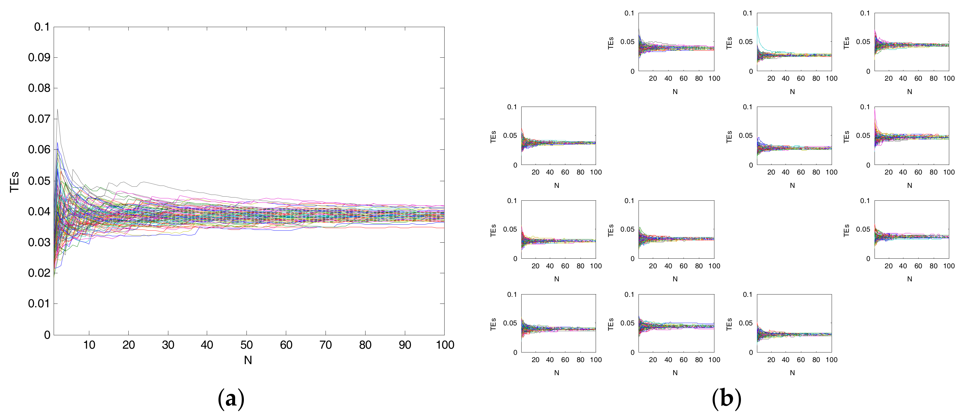
To determine the relationship between θT and the number of Monte Carlo simulations (N), another test with N = 1, 2, ···, 100 is applied, as shown in Figure 8. It is easy to see that when N > 40, the calculated θT is close to the actual threshold.
Based on the modified MI in Equation (6), the prediction horizon h of TE can be determined. Based on TE in Equation (4), the TEs between variables can be estimated. The null hypothesis is rejected if . Therefore, a significant causality can be detected between those variables. Based on the modified CMI in Equation (12), if (θI denotes the threshold for modified CMI), a direct causality from X to Y based on Z can be detected. Therefore, the process topology is obtained. To test the effectiveness of the proposed method, a numerical case and a simulated industrial case are given below.
6. Case Studies
This section gives a numerical example and a simulated industrial case, which can demonstrate the effectiveness of the proposed method.
6.1. Numerical Example
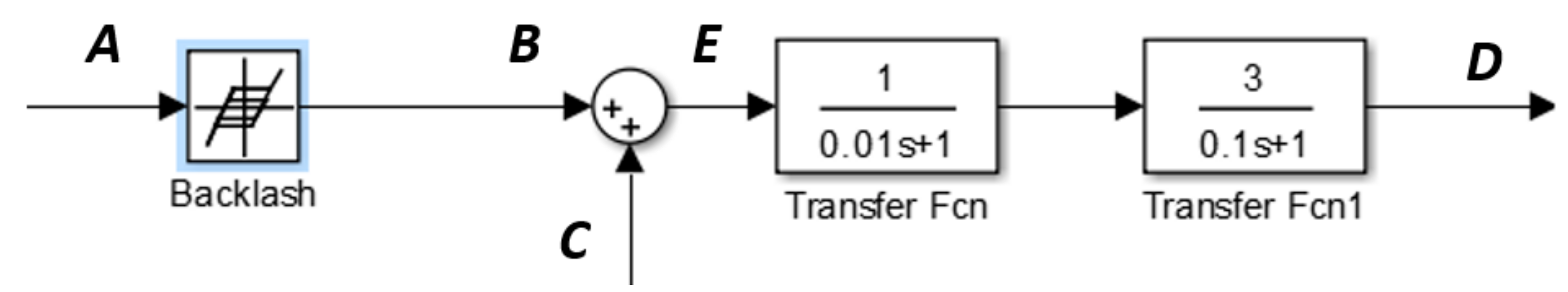
The first case is shown in Figure 9, where variables A and C are two uncorrelated random time series. There are three significant direct causality paths in the block diagram, which are from variable A to B and from variable B to D and variable C to D.
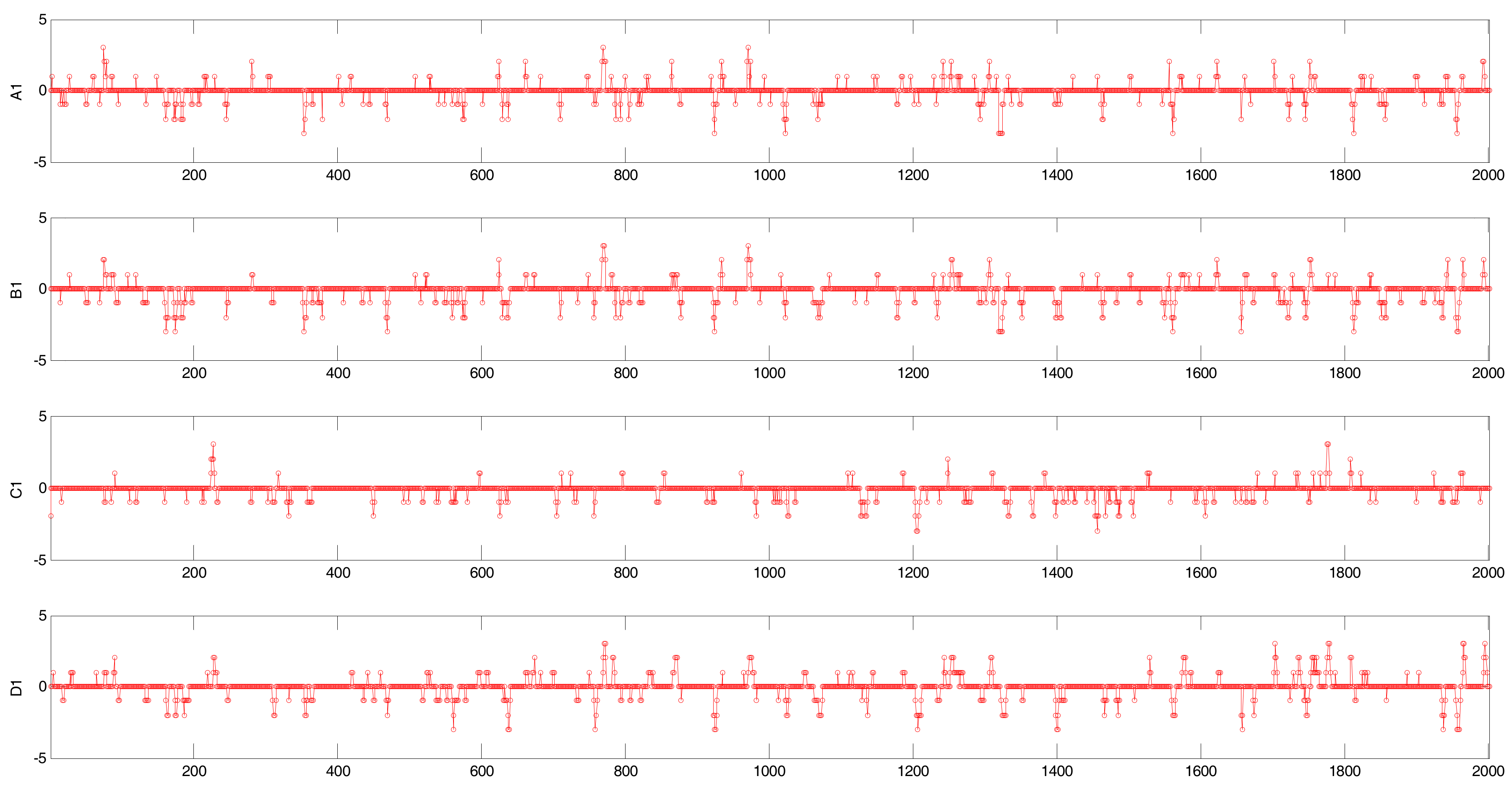
First, we convert the process data into binary alarm series with different thresholds for those variables. Considering the simulated model and the control requirements, we can choose the above-mentioned thresholds for those variables as shown in Figure 10. The simulated multi-valued alarm series A1, B1, C1, and D1 are generated by these variables as shown in Figure 11.
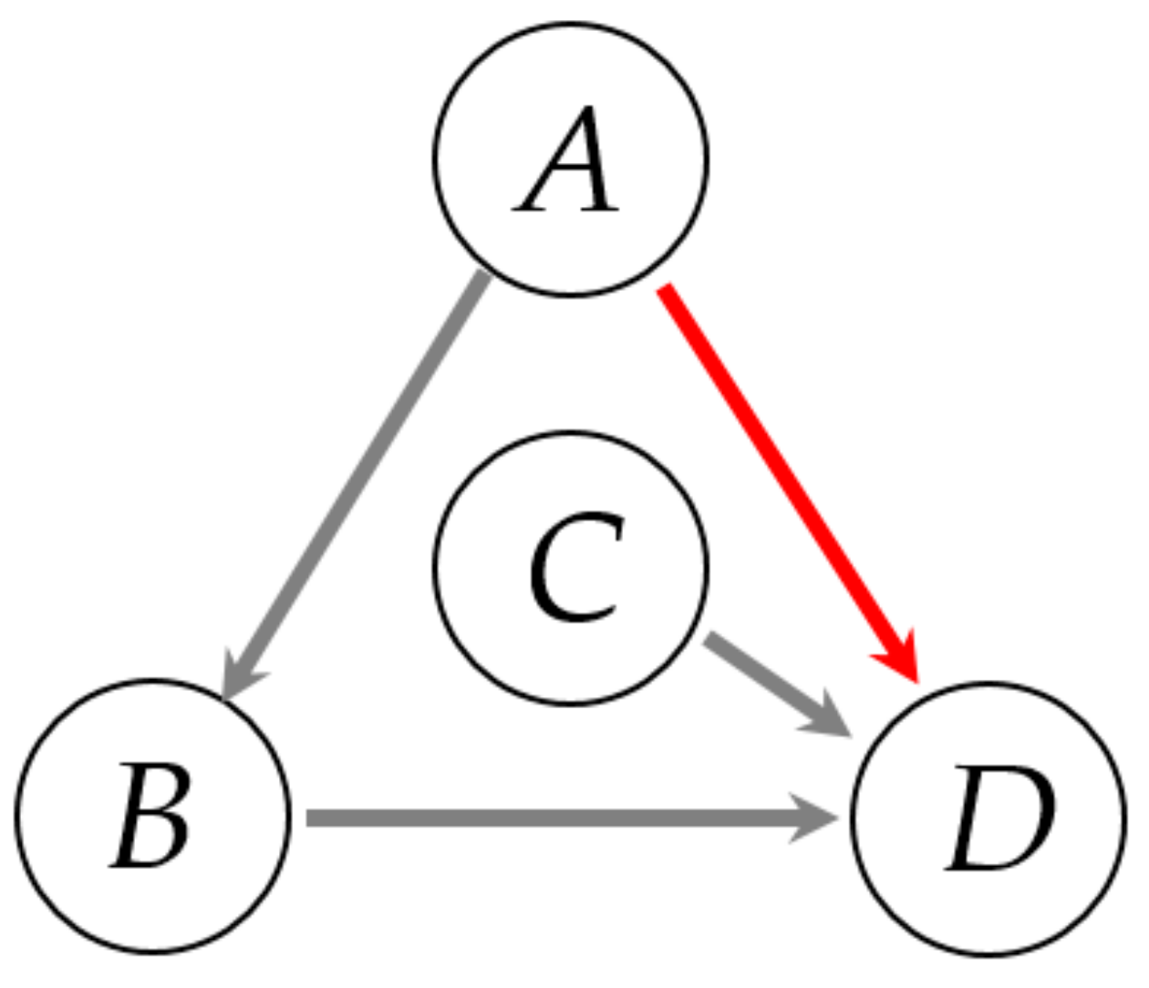
Second, based on the multi-valued alarm series in Figure 11, causality is captured according to Equation (4). The TEs and the corresponding significance thresholds (in the brackets) are shown in Table 2. The causality map based on Table 2 is shown in Figure 12.
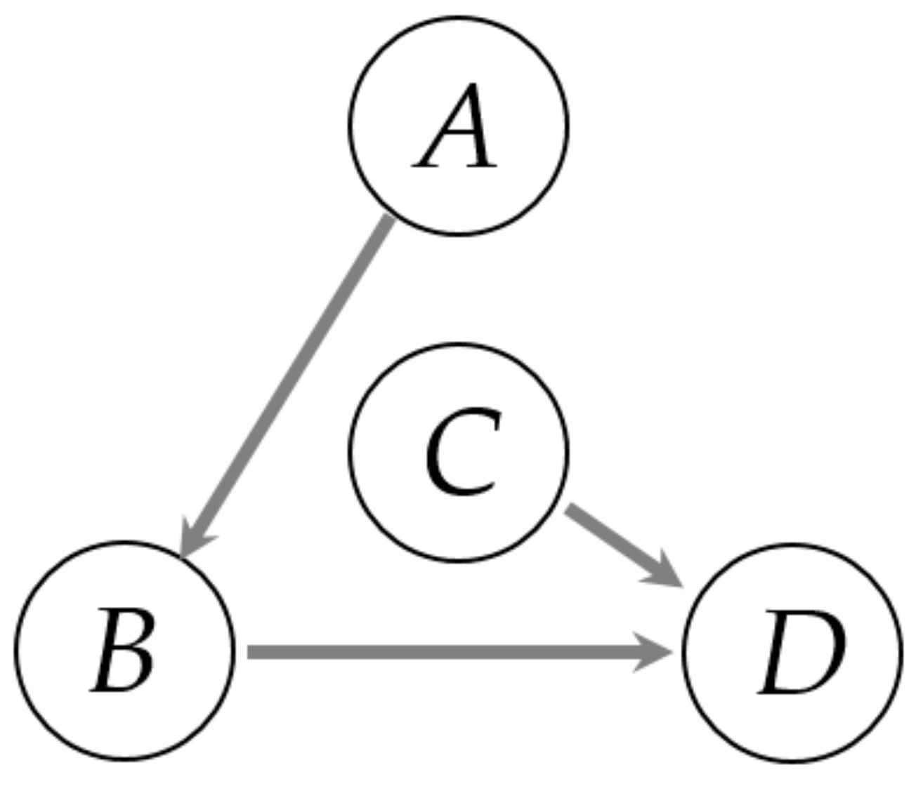
Then, all of the direct causal relationships in Table 2 can be identified by the modified CMI. In Figure 12, there are two links from A to D. One link is directly to D from A (A→D), and the other is from A to B to D (A→B→D). So, we need to determine whether the causality between A and D is direct or indirect through B. We obtain that 0.0416, and the corresponding significance threshold is according to the three-sigma rule. Since , we say that the causality from A to D is indirect. The real process topology between variables A, B, C, and D is shown in Figure 13 via the proposed method by using multi-valued alarm series. The results in Figure 13 are consistent with the above-mentioned simulated case in Figure 9. Based on this correct causal topology, a root cause analysis can be performed via a fault propagation analysis. For example, if a fault is detected in D, then B and C should be checked first; if B is ruled out, then A cannot be a root cause because there is no direct link from A to D.
6.2. Industrial Example
The benchmark Tennessee-Eastman Process [29], which was developed by Downs et al. as a simulation chemical process, is depicted in Figure 14. A decentralized control method was proposed to keep the simulated model in a normal operation situation [30], which is shown by dotted lines in Figure 14.
There are eight substances in the Tennessee–Eastman Process that are marked as A,B,C,D,E,F,G, and H in the following reaction equations
where A, B, C, and D are gaseous reactants which can be seen as blue circles in Figure 14; G and H are liquid products; B is an inert substance; and E and F are by-products. All reactions are exothermic and irreversible.
Four variables (stream 4, stream 10, level, and stream 11) are selected from the Tennessee–Eastman Process to demonstrate the proposed method’s performance. The multi-valued alarm series generated by those variables are shown in Figure 15. Then, the TEs via the proposed method and their corresponding significance thresholds (in brackets) are shown in Table 3.
In Figure 16, it is easy to see that there is a causal relationship between each pair of variables based on Table 3. TE cannot be used to distinguish indirect causality. Then, the modified CMI is used to determine direct causality between each pair of variables at different conditions from the causality map in Figure 16. A part of the CMIs and their corresponding significance thresholds (in brackets) is shown in Table 4.
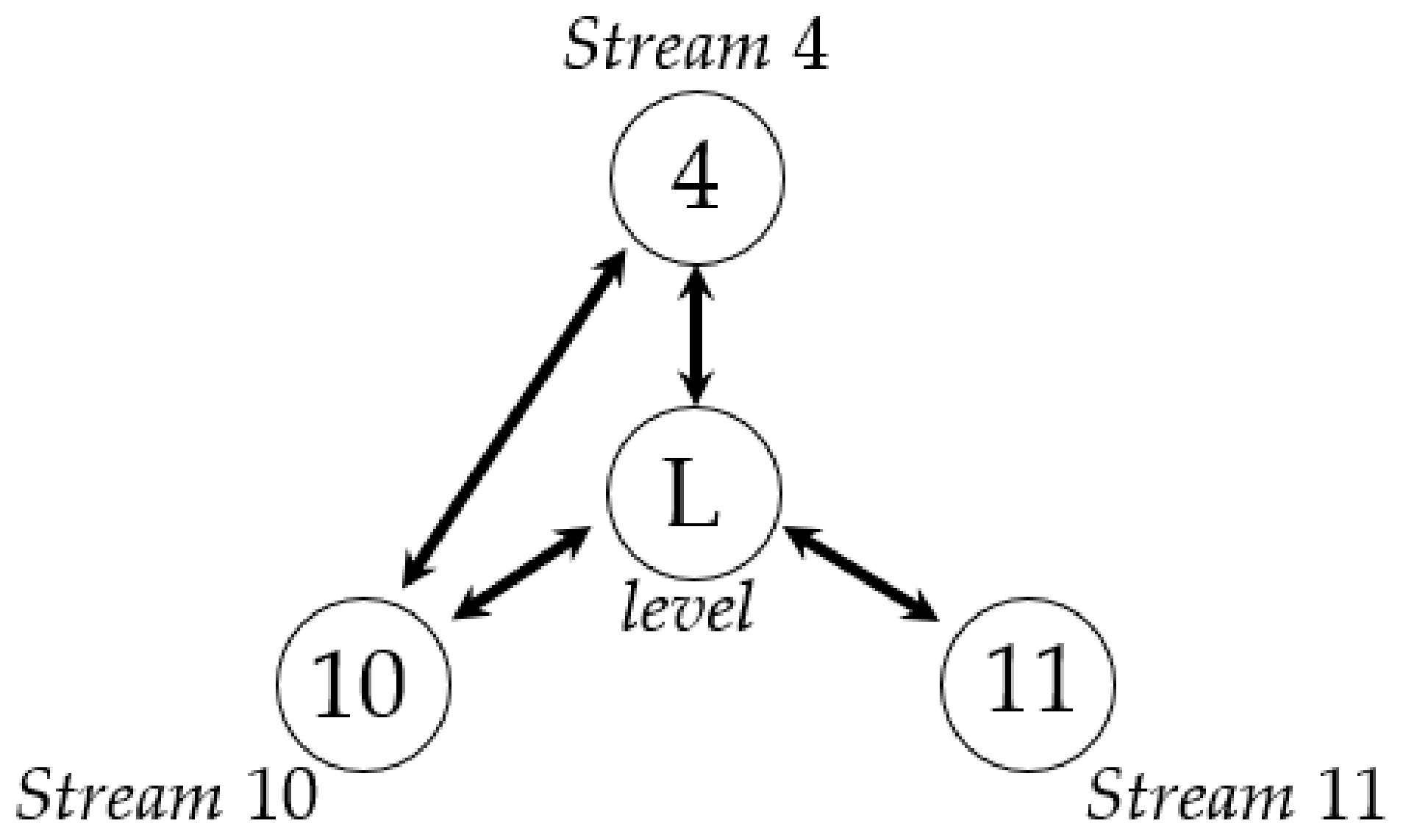
In Table 4, there is no direct causality between stream 4 and stream 10 and between stream 4 and stream 11. The process topology is that indirect causality is excluded, as shown in Figure 17. Considering the Tennessee–Eastman Process model and the control scheme, the results are consistent with the underlying model of the Tennessee–Eastman Process. In addition, the proposed method can be used to capture a direct causality map not only in the intelligent equipment and industrial system fields, but also in other fields, especially in the field of cloud platform anomaly detection. As we all know, with an increasing number of events or alarms on the cloud platform, we find that it is difficult to analyze the root cause promptly. Those events or alarms usually have several levels, which fit the proposed multi-valued series. Fortunately, the proposed method provides us with a new way to capture anomaly patterns on the cloud platform.
7. Conclusions
With the progress of science and technology, our society has become an information society. This brings new challenges to understand such information around us. Among the various types of information, alarms can directly give information about abnormalities. Given a large collection of temporal alarms, we can quickly and accurately find alarm patterns that lead to a certain type of alarm using the proposed method.
This is the first time multi-valued alarm series have been used to detect causality, notwithstanding that other types of data have been widely used. However, for the reason mentioned in Section 2, multi-valued alarm series are comparatively useful and ought to receive more attention. In this paper, to obtain a concise process topology excluding indirect causality, a hybrid method of TE and modified CMI is proposed using multi-valued alarm series. The transfer entropy method is used to obtain a causality map between all sub-processes, and the modified CMI method is used to distinguish direct connectivity from indirect connectivity based on modified alarm series (multi-valued alarm series).
The proposed multi-valued alarm series makes a huge difference in causality detection. The estimation of PDF based on this type of data is as computational-friendly as that based on binary alarm series. However, the proposed multi-valued alarm series increases the information of the alarm series and reduces the chance of error.
Because of the wide application prospects of the proposed multi-valued series and the low computational cost, the research and application of this type of data have reasonable significance. It can be used for fault propagation analyses in real industrial processes.
Acknowledgments
We would like to express our acknowledgements to the National Natural Science Foundation of China (61433001).
Author Contributions
Jianjun Su initiated the basic idea in the application background. Dezheng Wang formulated the problem, did all the experiments, and prepared the first draft under the supervision of Fan Yang and Yinong Zhang, who corrected and improved it. Yan Zhao and Xiangkun Pang participated in the discussion. All authors have read and approved the final manuscript.
Conflicts of Interest
The authors declare no conflict of interest.
References
- Yang, F.; Duan, P.; Shah, S.L.; Chen, T.W. Capturing Causality from Process Data. In Capturing Connectivity and Causality in Complex Industrial Processes; Springer: New York, NY, USA, 2014; pp. 57–62. [Google Scholar]
- Khandekar, S.; Muralidhar, K. Springerbriefs in applied sciences and technology. In Dropwise Condensation on Inclined Textured Surfaces; Springer: New York, NY, USA, 2014; pp. 17–72. [Google Scholar]
- Pant, G.B.; Rupa Kumar, K. Climates of south asia. Geogr. J. 1998, 164, 97–98. [Google Scholar]
- Donges, J.F.; Zou, Y.; Marwan, N.; Kurths, J. Complex networks in climate dynamics. Eur. Phys. J. Spec. Top. 2009, 174, 157–179. [Google Scholar] [CrossRef]
- Hiemstra, C.; Jones, J.D. Testing for linear and nonlinear granger causality in the stock price-volume relation. J. Financ. 1994, 49, 1639–1664. [Google Scholar]
- Wang, W.X.; Yang, R.; Lai, Y.C.; Kovanis, V.; Grebogi, C. Predicting catastrophes in nonlinear dynamical systems by compressive sensing. Phys. Rev. Lett. 2011, 106, 154101. [Google Scholar] [CrossRef] [PubMed]
- Hlavackova-Schindler, K.; Palus, M.; Vejmelka, M.; Bhattacharya, J. Causality detection based on information. Phys. Rep. 2007, 441. [Google Scholar] [CrossRef]
- Duggento, A.; Bianciardi, M.; Passamonti, L.; Wald, L.L.; Guerrisi, M.; Barbieri, R.; Toschi, N. Globally conditioned granger causality in brain-brain and brain-heart interactions: A combined heart rate variability/ultra-high-field (7 t) functional magnetic resonance imaging study. Philos. Trans. R. Soc. A Math. Phys. Eng. Sci. 2016, 374. [Google Scholar] [CrossRef] [PubMed]
- Liu, Y.-K.; Wu, G.-H.; Xie, C.-L.; Duan, Z.-Y.; Peng, M.-J.; Li, M.-K. A fault diagnosis method based on signed directed graph and matrix for nuclear power plants. Nucl. Eng. Des. 2016, 297, 166–174. [Google Scholar] [CrossRef]
- Maurya, M.R.; Rengaswamy, R.; Venkatasubramanian, V. A systematic framework for the development and analysis of signed digraphs for chemical processes. 2. Control loops and flowsheet analysis. Ind. Eng. Chem. Res. 2003, 42, 4811–4827. [Google Scholar] [CrossRef]
- Bauer, M.; Thornhill, N.F. A practical method for identifying the propagation path of plant-wide disturbances. J. Process Control 2008, 18, 707–719. [Google Scholar] [CrossRef]
- Chen, W.; Larrabee, B.R.; Ovsyannikova, I.G.; Kennedy, R.B.; Haralambieva, I.H.; Poland, G.A.; Schaid, D.J. Fine mapping causal variants with an approximate bayesian method using marginal test statistics. Genetics 2015, 200, 719–736. [Google Scholar] [CrossRef] [PubMed]
- Ghysels, E.; Hill, J.B.; Motegi, K. Testing for granger causality with mixed frequency data. J. Econom. 2016, 192, 207–230. [Google Scholar] [CrossRef]
- Yang, F.; Fan, N.J.; Ye, H. Application of PDC method in causality analysis of chemical process variables. J. Tsinghua Univ. (Sci. Technol.) 2013, 210–214. [Google Scholar]
- Bauer, M.; Cox, J.W.; Caveness, M.H.; Downs, J.J. Finding the direction of disturbance propagation in a chemical process using transfer entropy. IEEE Trans. Control Syst. Technol. 2007, 15, 12–21. [Google Scholar] [CrossRef] [Green Version]
- Duan, P.; Yang, F.; Chen, T.; Shah, S.L. Direct causality detection via the transfer entropy approach. IEEE Trans. Control Syst. Technol. 2013, 21, 2052–2066. [Google Scholar] [CrossRef]
- Duan, P.; Yang, F.; Shah, S.L.; Chen, T. Transfer zero-entropy and its application for capturing cause and effect relationship between variables. IEEE Trans. Control Syst. Technol. 2015, 23, 855–867. [Google Scholar] [CrossRef]
- Staniek, M.; Lehnertz, K. Symbolic transfer entropy. Phys. Rev. Lett. 2008, 100, 158101. [Google Scholar] [CrossRef] [PubMed]
- Yu, W.; Yang, F. Detection of causality between process variables based on industrial alarm data using transfer entropy. Entropy 2015, 17, 5868–5887. [Google Scholar] [CrossRef]
- Yang, Z.; Wang, J.; Chen, T. Detection of correlated alarms based on similarity coefficients of binary data. IEEE Trans. Autom. Sci. Eng. 2013, 10, 1014–1025. [Google Scholar] [CrossRef]
- Yang, F.; Shah, S.L.; Xiao, D.; Chen, T. Improved correlation analysis and visualization of industrial alarm data. ISA Trans. 2012, 51, 499–506. [Google Scholar] [CrossRef] [PubMed]
- Schreiber, T. Measuring information transfer. Phys. Rev. Lett. 2000, 85, 461–464. [Google Scholar] [CrossRef] [PubMed]
- Dehnad, K. Density Estimation for Statistics and Data Analysis by Bernard Silverman; Chapman and Hall: London, UK, 1986; pp. 296–297. [Google Scholar]
- Cover, T. Information Theory and Statistics. In Proceedings of the IEEE-IMS Workshop on Information Theory and Statistics, Alexandria, VA, USA, 27–29 October 1994; p. 2. [Google Scholar]
- Cover, T.M.; Thomas, J.A. Elements of Information Theory; Tsinghua University Press: Beijing, China, 2003; pp. 1600–, 1601. [Google Scholar]
- Palus, M.; Komárek, V.; Hrncír, Z.; Sterbová, K. Synchronization as adjustment of information rates: Detection from bivariate time series. Phys. Rev. E Stat. Nonlinear Soft Matter Phys. 2001, 63, 046211. [Google Scholar] [CrossRef] [PubMed]
- Runge, J.; Heitzig, J.; Petoukhov, V.; Kurths, J. Escaping the curse of dimensionality in estimating multivariate transfer entropy. Phys. Rev. Lett. 2012, 108, 258701. [Google Scholar] [CrossRef] [PubMed]
- Kantz, H.; Schreiber, T. Nonlinear Time Series Analysis; Cambridge University Press: Cambridge, UK, 1997; p. 491. [Google Scholar]
- Downs, J.J.; Vogel, E.F. A plant-wide industrial process control problem. Comput. Chem. Eng. 1993, 17, 245–255. [Google Scholar] [CrossRef]
- Ricker, N.L. Decentralized control of the tennessee eastman challenge process. J. Process Control 1996, 6, 205–221. [Google Scholar] [CrossRef]
Figure 1.
The time series A (the upper) and B. The red lines are the upper limits (H) of the normal states.
Figure 1.
The time series A (the upper) and B. The red lines are the upper limits (H) of the normal states.

Figure 2.
The binary alarm series A (the red line) and B (the blue line) according to H. (“false” for a fault state while “true” for a normal state).
Figure 2.
The binary alarm series A (the red line) and B (the blue line) according to H. (“false” for a fault state while “true” for a normal state).
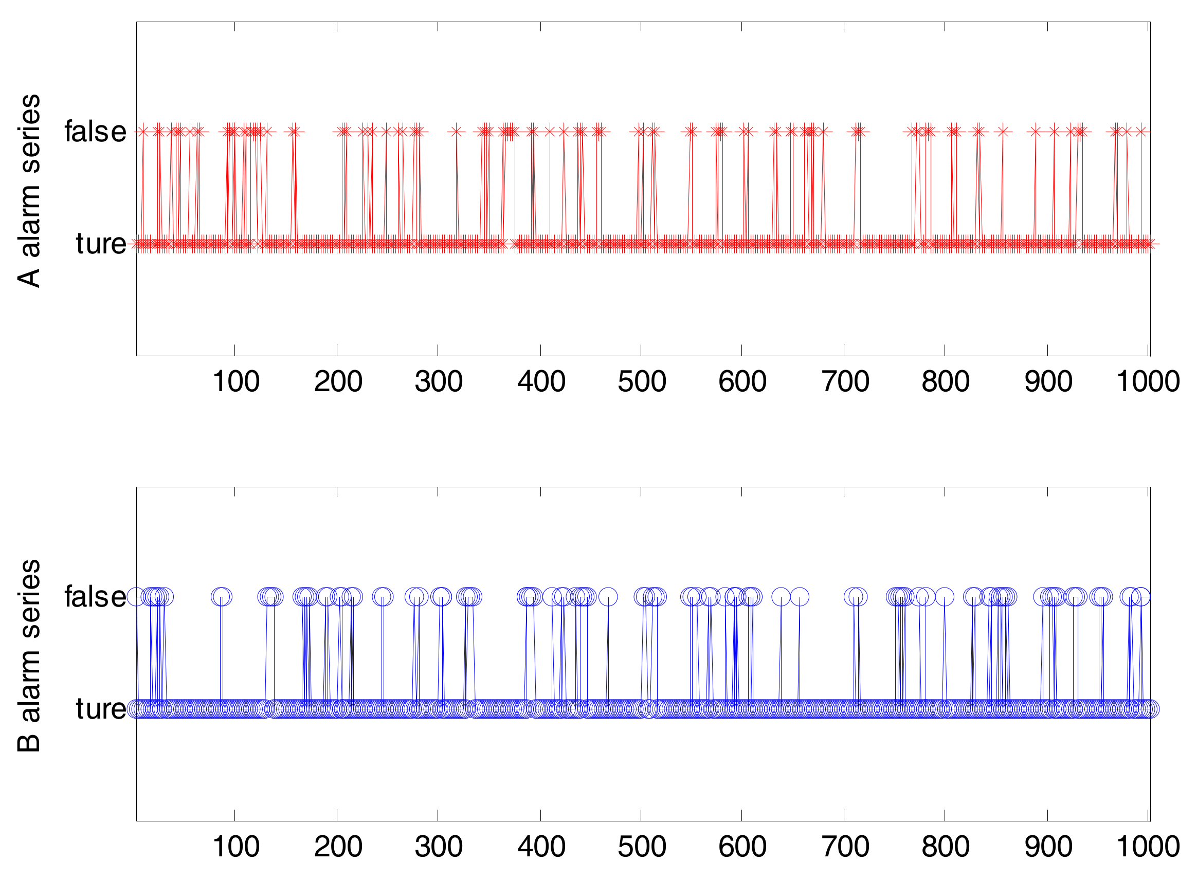
Figure 3.
Four types of alarms of MEAS_MON. U_AH denotes the high alarm limit (the threshold is chosen as 100); U_AL denotes the low alarm limit (the threshold is chosen as 0); U_WH denotes the high warning limit (the threshold is chosen as 95); and U_WL denotes the high alarm limit (the threshold is chosen as 5).
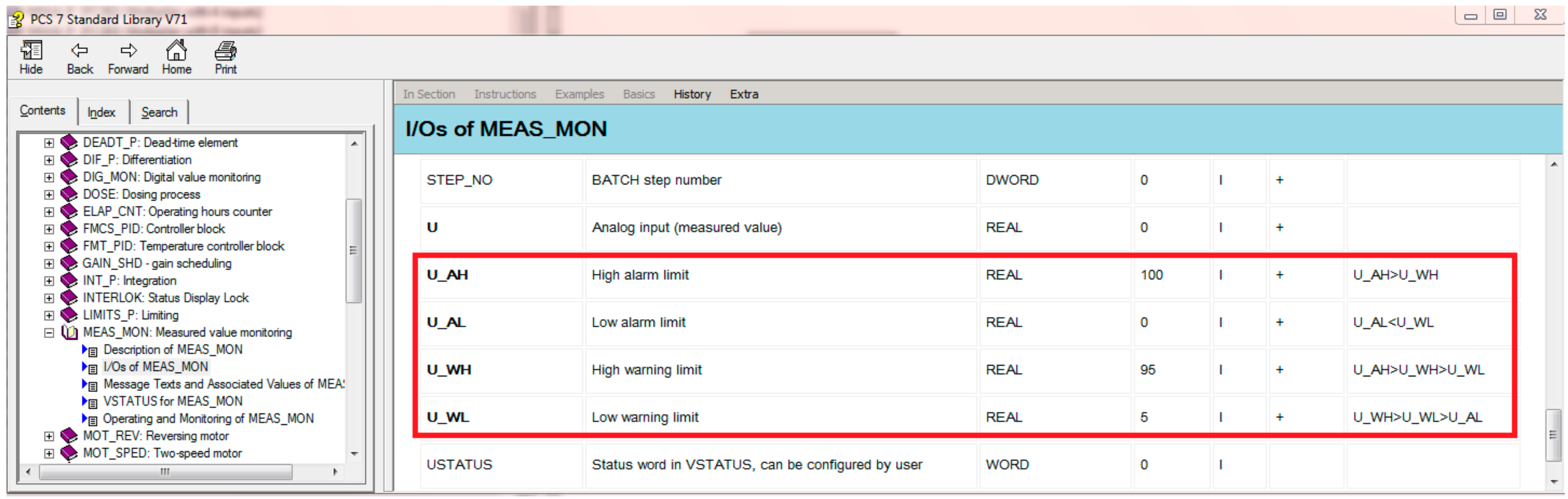
Figure 4.
Multi-valued alarm series. (a) shows the four alarm series (HI, LO, HH, LL) of A; (b) shows the four alarm series (HI, LO, HH, LL) of B; (c) shows the two multi-valued alarm series that is a combination of the four alarm series shown in Figure 4a,b, respectively. The multi-valued alarm series of A has three states and B has five states. HH: high alarm; HI: high warning; LO: low warning; LL: low alarm.
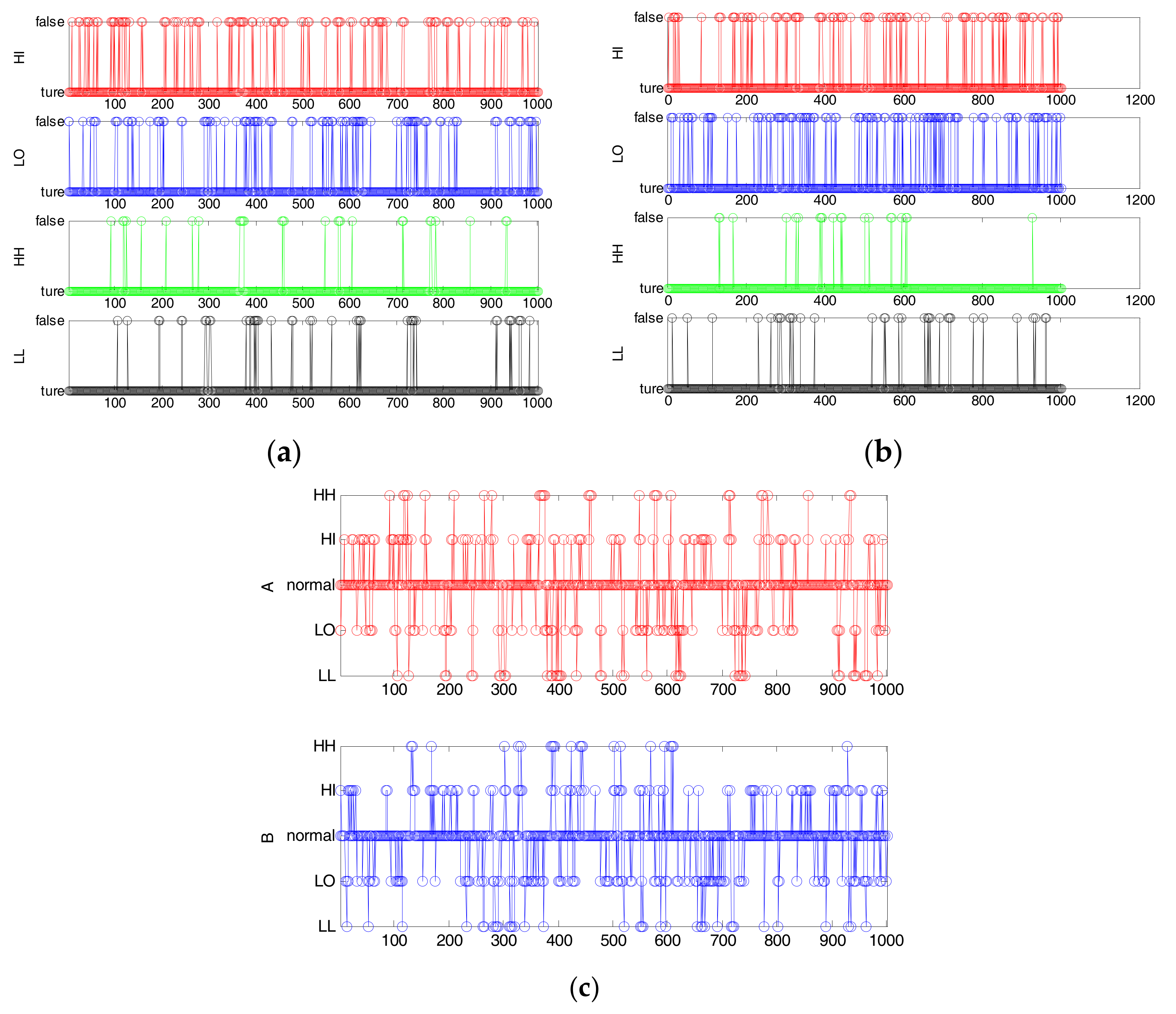
Figure 5.
Transfer entropy (TE) (red line) and modified mutual information (MI) (blue line) with different h.
Figure 5.
Transfer entropy (TE) (red line) and modified mutual information (MI) (blue line) with different h.
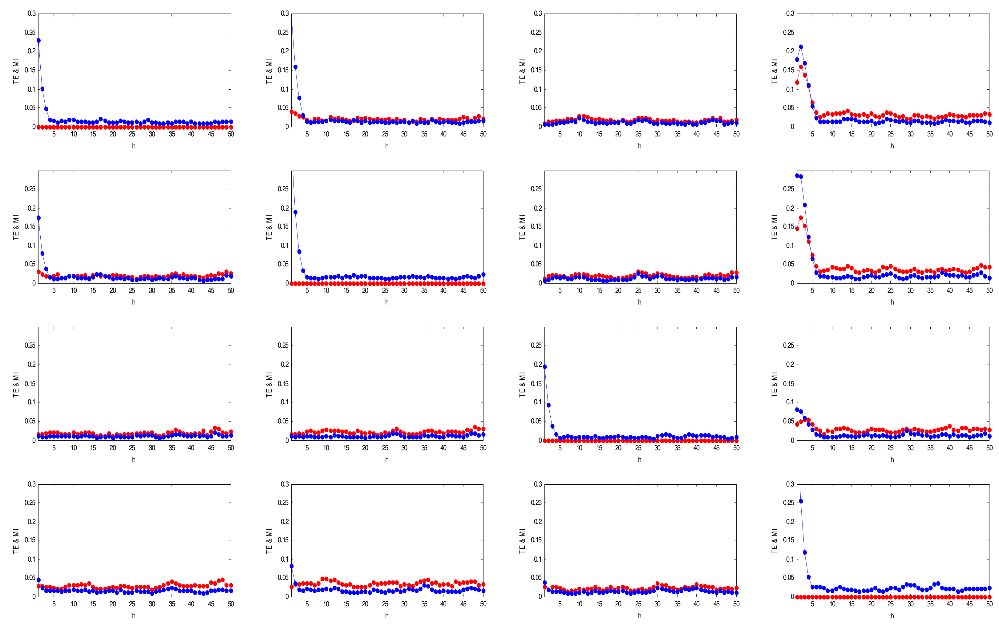
Figure 6.
TEs between variables A, B, C, D in Example 1 (to be analyzed later). The gray color indicates a true direct causality. The red color indicates an indirect causality.
Figure 6.
TEs between variables A, B, C, D in Example 1 (to be analyzed later). The gray color indicates a true direct causality. The red color indicates an indirect causality.
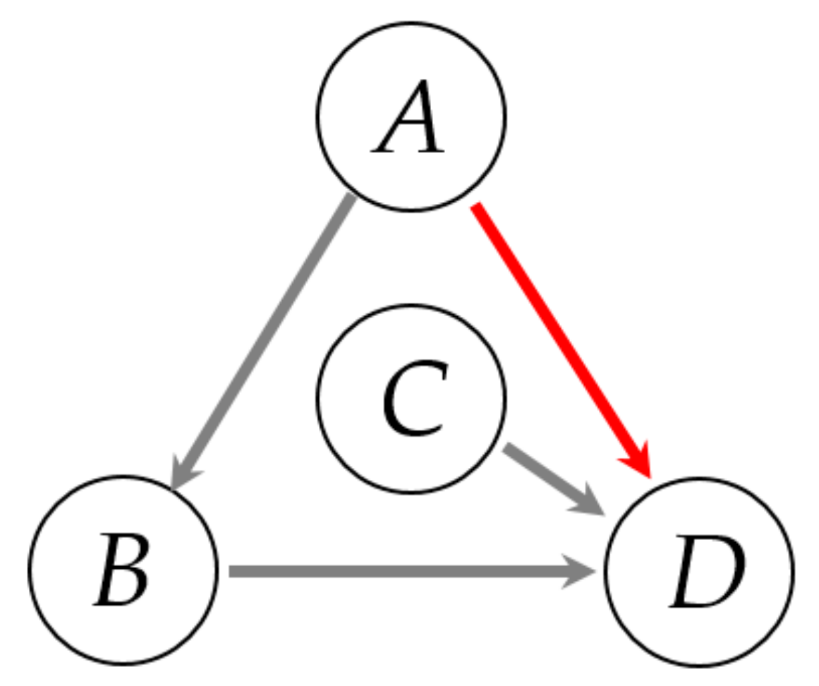
Figure 7.
N-trial Monte Carlo simulations. (a) TEs between variables stream 4 and stream 10; (b) TEs between all variables calculated from the surrogate data follow standard deviation.
Figure 7.
N-trial Monte Carlo simulations. (a) TEs between variables stream 4 and stream 10; (b) TEs between all variables calculated from the surrogate data follow standard deviation.
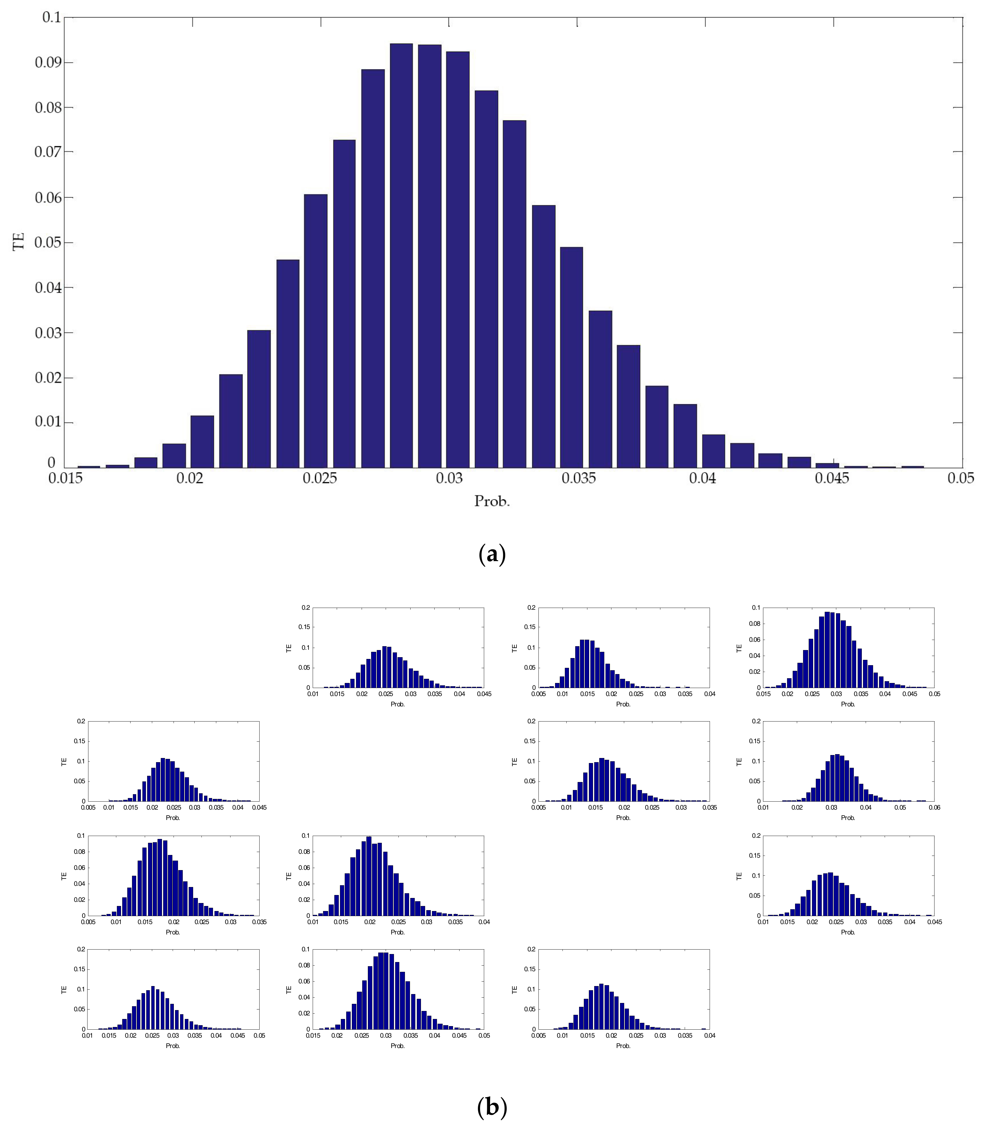
Figure 8.
The relationship between θ and N. (a) an example of 100 pairs of uncorrelated random series of a couple of variables; (b) an example of 100 pairs of uncorrelated random series of every couple of variables.
Figure 8.
The relationship between θ and N. (a) an example of 100 pairs of uncorrelated random series of a couple of variables; (b) an example of 100 pairs of uncorrelated random series of every couple of variables.

Figure 9.
Block diagram of a simulated example. Between A and B is a backlash block; E = B + C.

Figure 10.
Process data with thresholds. The most of states of each sequence is the normal state. It coincides with the real alarm situation very well. HHH: high error; LLL: low error.
Figure 10.
Process data with thresholds. The most of states of each sequence is the normal state. It coincides with the real alarm situation very well. HHH: high error; LLL: low error.
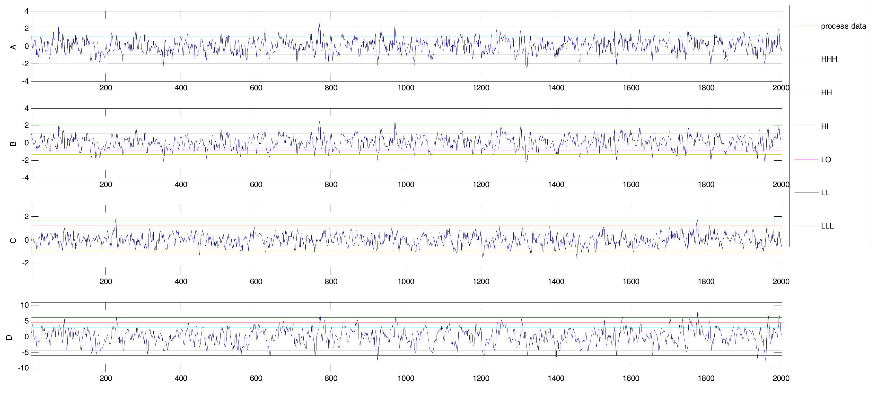
Figure 11.
Multi-valued alarm series: A1, B1, C1, and D1. The 0 denotes a normal state; 3 denotes high error (HHH); −3 denotes low error (LLL); −2 denotes HH; −2 denotes LL; 1 denotes HI; and −1 denotes LO.
Figure 11.
Multi-valued alarm series: A1, B1, C1, and D1. The 0 denotes a normal state; 3 denotes high error (HHH); −3 denotes low error (LLL); −2 denotes HH; −2 denotes LL; 1 denotes HI; and −1 denotes LO.

Figure 12.
(Color online) Causality map of all sub-processes. The red link denotes an indirect relationship.
Figure 12.
(Color online) Causality map of all sub-processes. The red link denotes an indirect relationship.

Figure 13.
Real process topology of the above-mentioned simulated case.

Figure 14.
Tennessee–Eastman Process and its control scheme [30]. The chosen variables are represented by red circles.
Figure 14.
Tennessee–Eastman Process and its control scheme [30]. The chosen variables are represented by red circles.
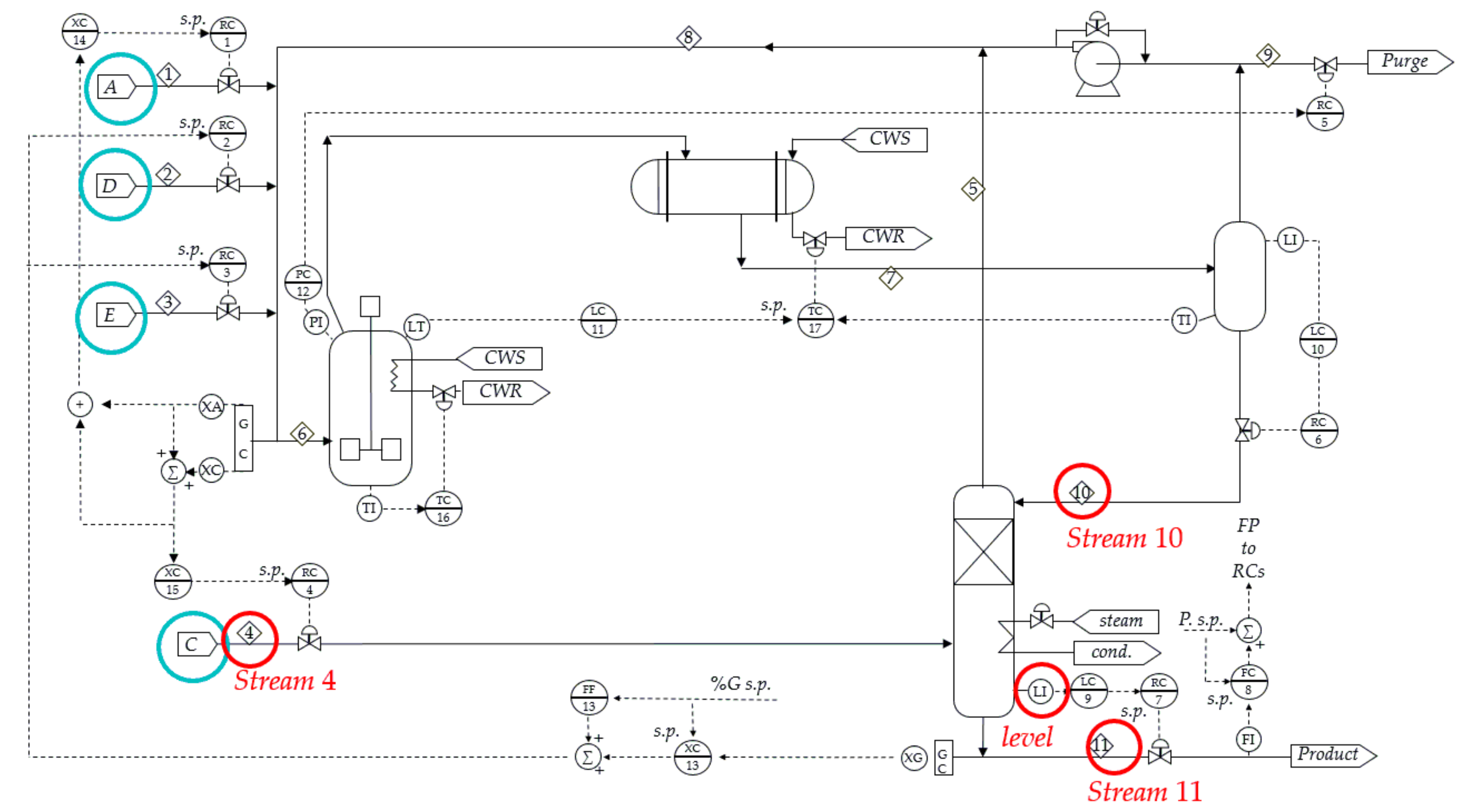
Figure 15.
Multi-valued alarm series of the Tennessee–Eastman Process case.
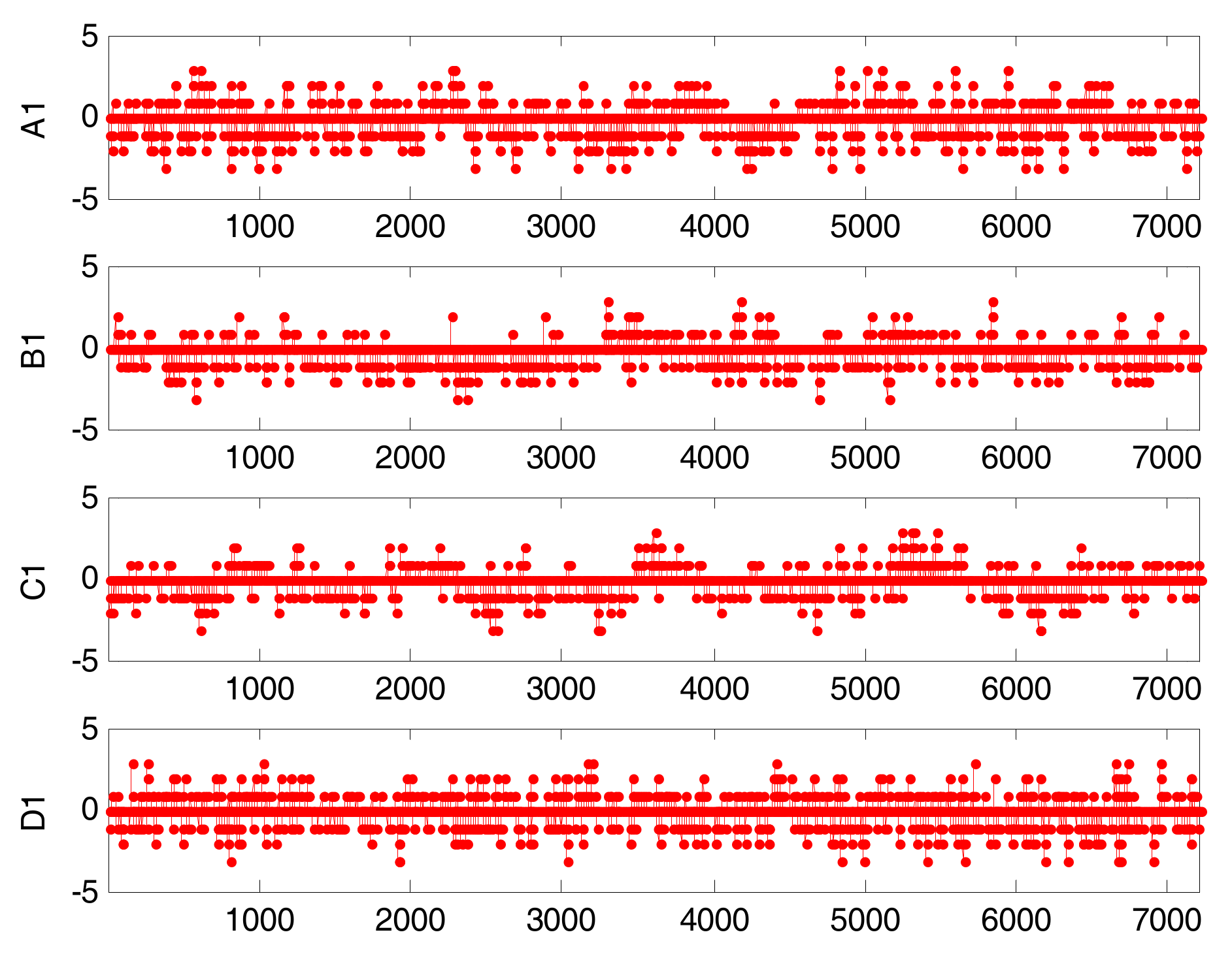
Figure 16.
Causality map of the Tennessee–Eastman Process case.
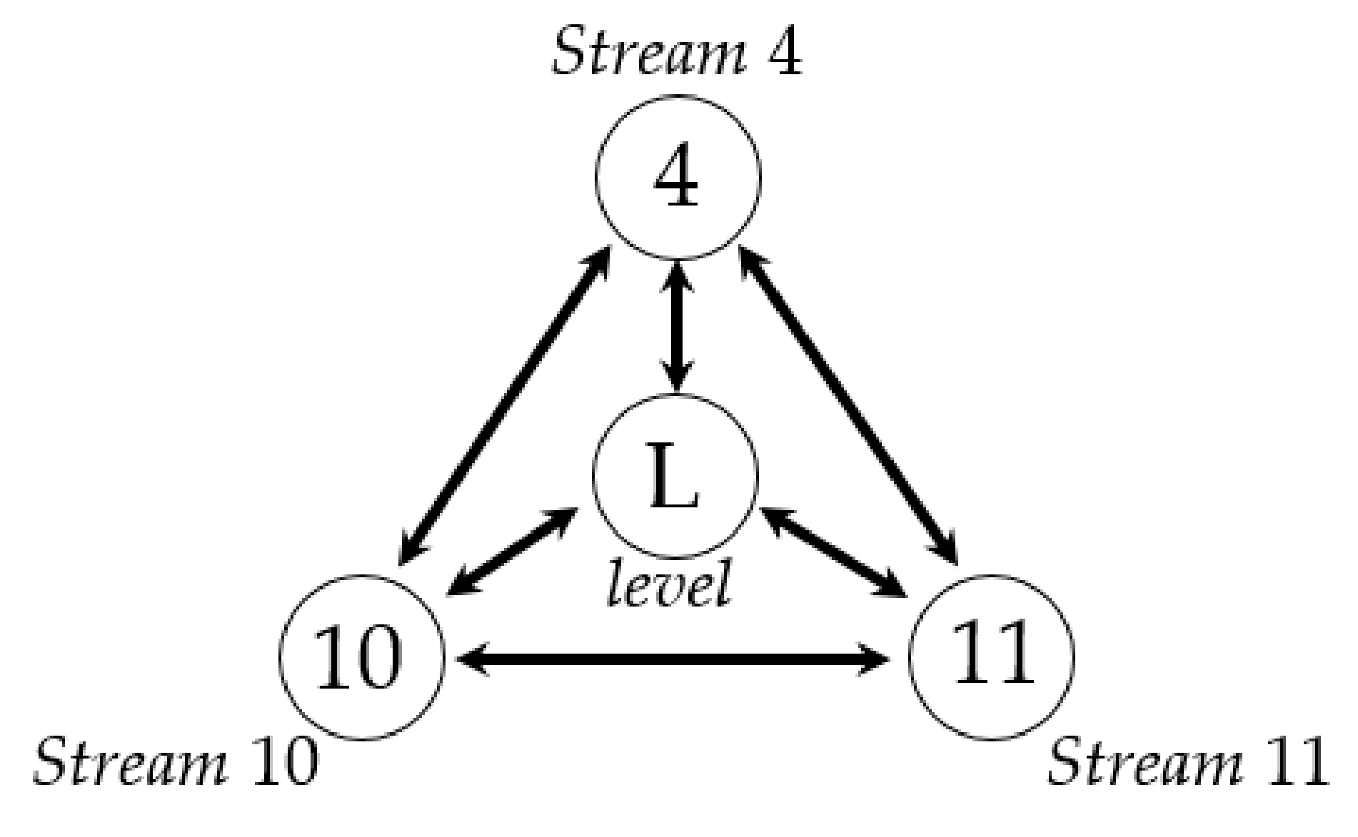
Figure 17.
Causality map of stream 4, stream 10, level, and stream 11.

Table 1.
Cross-correlation functions (CCFs) based on the three different series.
| CCF | Original Time Series | Binary Alarm Series | Multi-Valued Alarm Series |
|---|---|---|---|
| value | 0.15080 | 0.24580 | 0.14663 |
| Lag | 245 | −71 | 245 |
Table 2.
The TEs based on Example 1 by using multi-valued alarm series and their corresponding significance thresholds (in brackets).
Table 2.
The TEs based on Example 1 by using multi-valued alarm series and their corresponding significance thresholds (in brackets).
| To A | To B | To C | To D | |
|---|---|---|---|---|
| From A | - | 0.041(0.036) | 0.016(0.025) | 0.159(0.046) |
| From B | 0.031(0.035) | - | 0.021(0.026) | 0.175(0.049) |
| From C | 0.021(0.029) | 0.023(0.030) | - | 0.055(0.041) |
| From D | 0.028(0.037) | 0.035(0.045) | 0.027(0.030) |
Table 3.
TEs based on the Tennessee–Eastman Process example by using multi-valued alarm series and their corresponding significance thresholds (in brackets).
Table 3.
TEs based on the Tennessee–Eastman Process example by using multi-valued alarm series and their corresponding significance thresholds (in brackets).
| To Stream 4 | To Stream 10 | To Level | To Stream 11 | |
|---|---|---|---|---|
| From stream 4 | 0.456(0.027) | 0.290(0.025) | 0.182(0.019) | |
| From stream 10 | 0.379(0.028) | 0.423(0.021) | 0.257(0.016) | |
| From level | 0.028(0.027) | 0.289(0.022) | 0.139(0.015) | |
| From stream 11 | 0.152(0.023) | 0.030(0.019) | 0.035(0.018) |
Table 4.
Conditional mutual information (CMIs) and their corresponding significance thresholds (in brackets).
Table 4.
Conditional mutual information (CMIs) and their corresponding significance thresholds (in brackets).
| Condition | To Stream 4 | |
|---|---|---|
| From stream 11 | Stream 4 and level | 0.026(0.036) |
| From stream 11 | Stream 10 and level | 0.016(0.038) |
| From stream 10 | Stream 4 | 0.119(0.020) |
| From stream 10 | Stream 4 and stream 11 | 0.027(0.037) |
| From stream 4 | level | 0.018(0.021) |
© 2017 by the authors. Licensee MDPI, Basel, Switzerland. This article is an open access article distributed under the terms and conditions of the Creative Commons Attribution (CC BY) license (http://creativecommons.org/licenses/by/4.0/).
Share and Cite
MDPI and ACS Style
Su, J.; Wang, D.; Zhang, Y.; Yang, F.; Zhao, Y.; Pang, X. Capturing Causality for Fault Diagnosis Based on Multi-Valued Alarm Series Using Transfer Entropy. Entropy 2017, 19, 663. https://doi.org/10.3390/e19120663
AMA Style
Su J, Wang D, Zhang Y, Yang F, Zhao Y, Pang X. Capturing Causality for Fault Diagnosis Based on Multi-Valued Alarm Series Using Transfer Entropy. Entropy. 2017; 19(12):663. https://doi.org/10.3390/e19120663
Chicago/Turabian StyleSu, Jianjun, Dezheng Wang, Yinong Zhang, Fan Yang, Yan Zhao, and Xiangkun Pang. 2017. "Capturing Causality for Fault Diagnosis Based on Multi-Valued Alarm Series Using Transfer Entropy" Entropy 19, no. 12: 663. https://doi.org/10.3390/e19120663
Note that from the first issue of 2016, this journal uses article numbers instead of page numbers. See further details here.