L1-Minimization Algorithm for Bayesian Online Compressed Sensing

1
Latam Experian DataLab , São Paulo-SP 04547-130, Brazil
2
Department of General Physics, Institute of Physics, University of São Paulo, São Paulo-SP 05508-090, Brazil
3
Department of Applied Mathematics, Institute of Mathematics and Statistics, University of São Paulo, São Paulo-SP 05508-090, Brazil
*
Author to whom correspondence should be addressed.
Entropy 2017, 19(12), 667; https://doi.org/10.3390/e19120667
Submission received: 3 November 2017
/
Revised: 25 November 2017
/
Accepted: 1 December 2017
/
Published: 5 December 2017
(This article belongs to the Special Issue MaxEnt 2017 - The 37th International Workshop on Bayesian Inference and Maximum Entropy Methods in Science and Engineering)
Abstract
:In this work, we propose a Bayesian online reconstruction algorithm for sparse signals based on Compressed Sensing and inspired by L1-regularization schemes. A previous work has introduced a mean-field approximation for the Bayesian online algorithm and has shown that it is possible to saturate the offline performance in the presence of Gaussian measurement noise when the signal generating distribution is known. Here, we build on these results and show that reconstruction is possible even if prior knowledge about the generation of the signal is limited, by introduction of a Laplace prior and of an extra Kullback–Leibler divergence minimization step for hyper-parameter learning.
1. Introduction
It has become commonplace to talk about the recent “information explosion” or “data deluge”. These expressions refer to a much faster growth in data production compared to all available data storage and to the even more evident divergence between the volume of data produced and the general data processing capacity. This state of things begs for more efficient ways of storing and analyzing data. Natural and man-made signals tend to be compressible, which means their innate redundancies allow them to be expressed as a small number of combinations of its components—they are sparse in some basis. In the last few decades a lot of effort has been directed to the development of compression techniques that allow the sampled data to be rewritten to a reduced number of bits. However, these techniques mean superfluous costs on the gathering and processing of the data. When talking about medical imaging that includes radiation, unnecessary data gathering almost certainly signifies collateral and unwanted health effects in the long run for the patients.
Compressed sensing (CS) is a framework for signal processing that presents itself as a successful resource that has produced many techniques for efficient information extraction [1]. CS utilizes the fact that real-world signals can typically be represented by a small combination of elemental components [2,3] to eliminate the data redundancy directly in its acquisition (in contrast with what occurs in a digital camera, for example, that captures millions of point measurements each time a picture is taken only to discard a large portion of this data immediately after its acquisition through a image compression algorithm). In a standard scenario, CS utilizes the sparsity property to enable the recovery of various signals from much fewer samples of linear measurements than required by the Nyquist–Shannon theorem [4,5]. The Nyquist rate [6,7] is a concept present in virtually all signal acquisition protocols used in consumer electronics and medical imaging devices, among others [2]. Unfortunately, it implies the necessity of a high sampling frequency, which means an especially high demand if we consider the now pervasive high definition registers. Between 2004 and 2006, Candès, Tao and Donoho [4,8,9] showed that sparse signals could be exactly reconstructed with below-the-Nyquist-rate sampling. Moreover (and perhaps what made it so intriguing), the reconstruction could be done in non-adaptive fashion through L1-minimization. These seminal works gave rise to CS [5]. It should be noted that “sampling” here has a twist, though, in CS, a sample of the signal is obtained by calculating its inner product against different test functions. All in all, the popularity of CS in the last few years made it pervasive through various disciplines, from Computer Science to Statistical Physics.
In this work, we consider the scenario of a signal generated by an unknown distribution and its recovery by means of a Bayesian online CS scheme. There is a vast literature on Bayesian schemes for CS (e.g., [10,11,12]) and their reconstruction have been thoroughly examined, not least by the Statistical Physics community [13,14,15]. Online reconstruction schemes can be invaluable in situations where real-time inference is needed (e.g., magnetic resonance imaging), when the data set is too large to be entirely stored on a hard disk (e.g., modern simulation science) or in the presence of time-variant signals (e.g., data streaming). Algorithms for Bayesian online learning are well-known in the neural networks community [16,17,18] and, in many fields of engineering such as optimal control theory, where they are known as Kalman filters [19,20,21]. In addition, an interesting compromise between online and offline learning is the so-called mini-batch learning [22], which has recently also found its way to the CS scenario [23]. In direct connection with this letter, previous work [24] has already established the possibility of online CS reconstruction, but it suffered from an important limitation, namely the necessity of an exact knowledge about the generating distribution of the signal.
This paper is organized as follows: in Section 2, the basic CS problem is defined, together with two reconstruction methods—the L1-minimization problem called LASSO (Least Absolute Shrinkage and Selection Operator) and the Bayesian scheme. Section 3 introduces the Bayesian online CS framework as presented in [24]. In Section 4, the main contribution of this work, an extension for the online framework in which imperfect knowledge about the signal generating distribution is allowed, is described. Section 5 presents the main results and Section 6 summarizes and discusses the main findings of this work.
2. Problem Setup
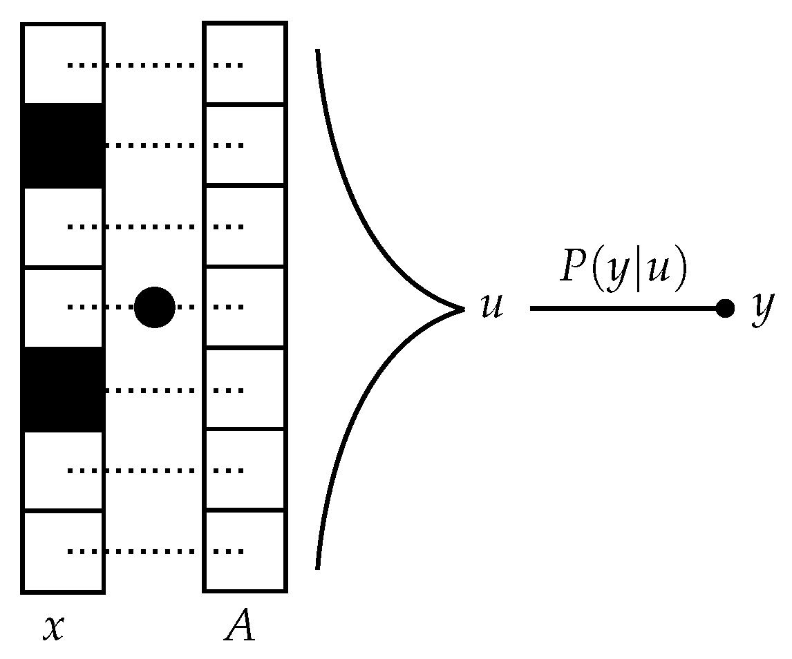
Let be a real N-dimensional signal where each component is generated by a sparsity-inducing distribution . It is assumed that and that does not have a finite mass at the origin. Sequential linear projections of the signal with known independent random measurement vectors , with are obtained at instants . Let these random projections pass through a (possibly noisy) channel before their result becomes available—this way, the value of each measurement, , will be distributed according to (Figure 1).
A common goal in Compressed Sensing is to accurately recover the signal based on the knowledge of and of the functional form of the channel . Since the beginnings of CS, the staple technique in the field [5] has been the LASSO, an optimization problem with an L1-regularization term [25],
where , is a matrix with all vectors as rows and the Lp-norms are defined as . The seminal works [4,8,9] were pivotal in proving that perfect signal reconstruction in absence of noise is possible by means of (1) even in subsampling scenarios (i.e., for , with ) . The Statistical Physics community is no stranger for these results, with typical behaviour analysis for large systems, where [26,27] being accepted as guarantees for the validity of the method.
3. Bayesian Online Compressed Sensing
In this work, reconstruction of the signal is done in an online manner. That is, measurements are used one at a time and discarded thereafter (in opposition to the offline/batch scenarios presented above where the whole dataset is available during the entire reconstruction). In addition, we would like to achieve this objective with limited knowledge about the generating distribution .
Bayes’ Theorem (2) can be easily transformed into an online update recursion [16]. Since all measurements are independent by design, the likelihood can be factored as
This way, the posterior distribution for the signal after t measurements can be written
In general, distribution can be complicated, so the calculation of is potentially difficult. Consider for now the Compressed Sensing scenario where the prior distribution is exactly the same as the known signal generating distribution . The factor here adds a singularity to the prior , so that the posterior should not approximate a Gaussian distribution even for , which was a crucial hypothesis in previous works [16] and would greatly simplify asymptotic calculations. In absence of such a simplification, a previous work [24] introduced the following mean-field approximation:
for the posterior distribution in Label (5) as a device to facilitate marginal computations and (as a consequence) their expected values. In this expression, is a set of natural parameters and
is the normalization of the marginal distribution , where denotes integration over all . So as not to introduce any biases, we define , which results in . The mmse estimate of the signal and its variance can then be readily calculated from the approximate posterior as
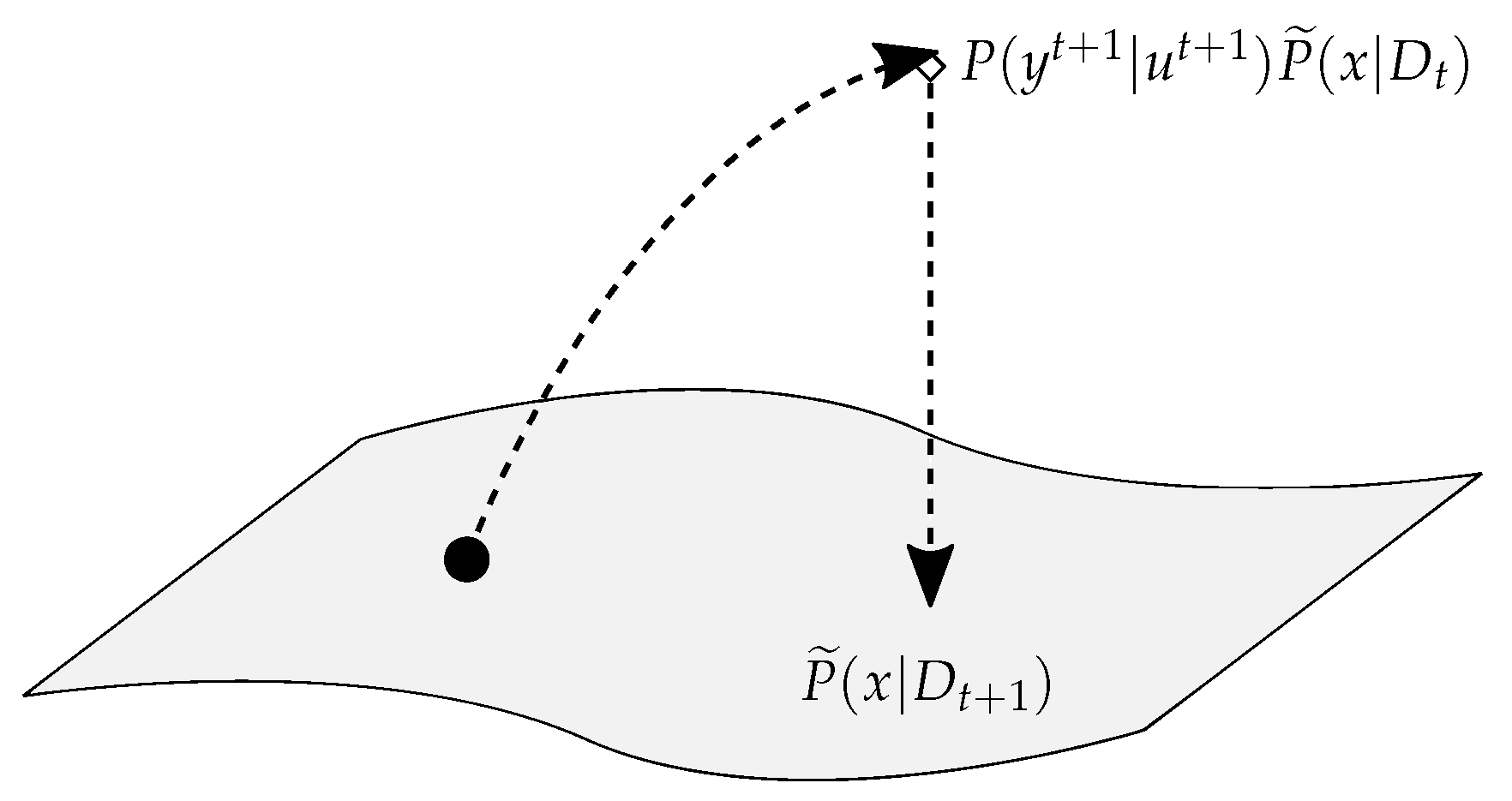
respectively. Equations (5) and (6) correspond to a sequence of update and projection steps—the update step adds new information obtained with the most recent measurement t, but transforms the posterior into a possibly intractable distribution; the projection step then returns this distribution to an easier exponential representation with independent components (Figure 2). The full scheme can be summarized as update rules for the parameters [24]. Defining and , these rules are
where and is the standard Gaussian measure. It has been shown [24] that this online algorithm has an asymptotic error decay comparable to the offline reconstruction scheme when additive measurement noise is present. In the noiseless scenario, the offline Bayesian algorithm achieves zero error for finite t, while the online version decays exponentially.
4. Mismatched Priors and L1-Minimization Based Reconstruction
A limitation of the framework introduced above is the simple fact that, in a real-world scenario, one does not know the exact parameters of the generating distribution, and possibly not even some of its major characteristics except for the fact that the generated signals are somewhat sparse. Using this algorithm as a canvas, we propose a strategy based on a Bayesian formulation of the L1-regularized problem, relying on the use of the sparsity-inducing Laplace prior
and a learning scheme for concurrent with the measurements. The use of Laplace-like priors is not new in the literature [29,30,31], but, to the best of our knowledge, this has not been introduced as part of an online algorithm yet.
We observe that the L1-estimator (1) can also be written in a Bayesian manner as , where
with a normalization factor dependent on and . This formulation suggests the replacement of the generating distribution in Label (6) for , effectively altering the projection step of the Bayesian online algorithm to the similar expression
where . The first and second moments of this alternate approximate distribution are, respectively,
paralleling Equations (8) and (9). Note that the natural parameters update Equations (10) and (11) remain unchanged, since they are independent of our choice of prior, be it , , or any other.
A common practical issue when making use of the L1-regularization scheme (1) is that the best value of the shrinkage parameter is data-dependent and not always clear. Nevertheless, its value is highly influential on the reconstructed model—there is a direct relation between and the number of non-zero coefficients in the estimate, which is reflected on the prediction accuracy of the model [32]. Therefore, since it is crucial to estimate accurate values of the shrinkage parameter, usual strategies in offline scenarios include calculation of its best value through cross-validation procedures [25] or straight calculation of an ideal number of non-zero covariates by adding one at a time in a recursive manner [32]. Unfortunately, these strategies are of little use in our present setting, where each measurement has to be used only once in an online manner.
Given any two distributions and , the Kullback–Leibler divergence [33], is a common measure for their dissimilarity. Also called relative entropy, it has the interesting property that always and it is zero if and only if . Now, whenever distribution is of the exponential family, i.e., , minimization of with respect to is equivalent to matching the moments and . In particular, for the exact posterior P as defined in the left-hand side of Label (2), minimization of with respect to after measurement t, i.e., finding such that
is the same as solving the implicit equation
for . Here, is the best possible estimate for the true sparsity of the original signal, . Our proposal is that is, at any instant t, an optimal estimate for the shrinkage parameter. Moreover, it is not static. With the natural parameters evolving, must change as well to maintain .
Alas, the left-hand side of expression (18) is unknown. To overcome this difficulty, we make the approximation . An argument can be made in its defense: as more and more measurements are acquired and the approximate posterior distribution (14) concentrates around the true values, two limits are obtained: (a) and (b) . The first limit has been proved in the large signal size limit in [24] for an exact prior; here, we assume its validity also in the present scenario. As for the second limit, Minkowski inequality guarantees that ; with the collapse of the distribution around the true value at , no probability mass crosses the axis, so that the equality limit is met. Therefore, these results mean a good estimate for the solution of (18) is given by that solves
for , where the right-hand side can be directly calculated from . This implicit expression corresponds to an extra step in the online algorithm for the recovery of the signal, which is shown in full below (Algorithm 1).
| Algorithm 1 Online -based signal recovery for CS. | |
| 1: Initialize | ▹; |
| 2: while do | |
| 3: Obtain new measurement | |
| 4: Update | ▹ Equations (10) and (11) |
| 5: Find | ▹ Equation (19) |
| 6: Update | |
| 7: Estimate signal means and variances | ▹ Equations (15) and (16) |
| 8: end while | |
| 9: return | |
5. Results and Discussion
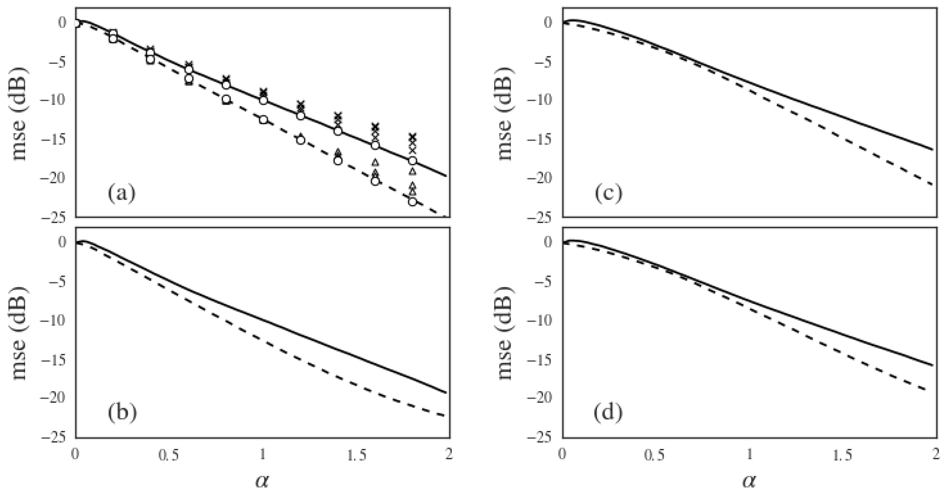
We tested the algorithm on sparse signals generated by two different distributions of the form , with . The factor induces sparsity by making every component equal to zero with probability . The non-sparse components could either come from a Gaussian distribution or from a binary distribution . To better evaluate the accuracy losses incurred due to approximation (19), we also tested the algorithm for the ideal situation where is known. To guarantee practical usefulness, all results correspond to the standard CS scenario with Gaussian noise , i.e., . Its noiseless counterpart can be obtained by taking the limit , which leads to . Figure 3 shows the average mean squared error normalized by resulting of simulations of the L1-based online CS algorithm with learning. Simulations for finite signal length size N showed decreasing error for increasing N—in order to correct for finite size effects, the curves in Figure 3 were obtained by extrapolating the results for finite and 2000 to by means of a quadratic fit. As expected, approximation (19) induces a significant accuracy loss, but, for , the reconstruction error decays approximately exponentially, proving the usefulness of the reconstruction scheme.
In all the examples shown, the solution to Equation (19) was obtained by numerically searching the value which best approximates both sides, i.e., by finding . The empirical results prove what could have been a reasonable assumption: Figure 4 shows that in the early stages when only a few measurements have been obtained, even for an exact prior, is not an excellent approximation of . It also shows that the approximation gets progressively better with more measurements. For this reason, we found that the use of a small damping factor in the update of provides faster and more accurate learning.
Finding an optimal value for the sparsity-inducing parameter is not trivial. Ideally, one desires to find such that the would represent the actual sparsity of the original signal . The limit is undesirable, since the soft constraints in due to the finite value of the natural parameters would not be enough to prevent the prior distribution to completely dominate the entire approximate posterior, leading all signal estimates to zero. At the same time, consider as a representative example the update Equations (10) and (11) for the noisy standard CS scenario, which can explicitly written as and . Taking the average of and over the measurement vectors results in
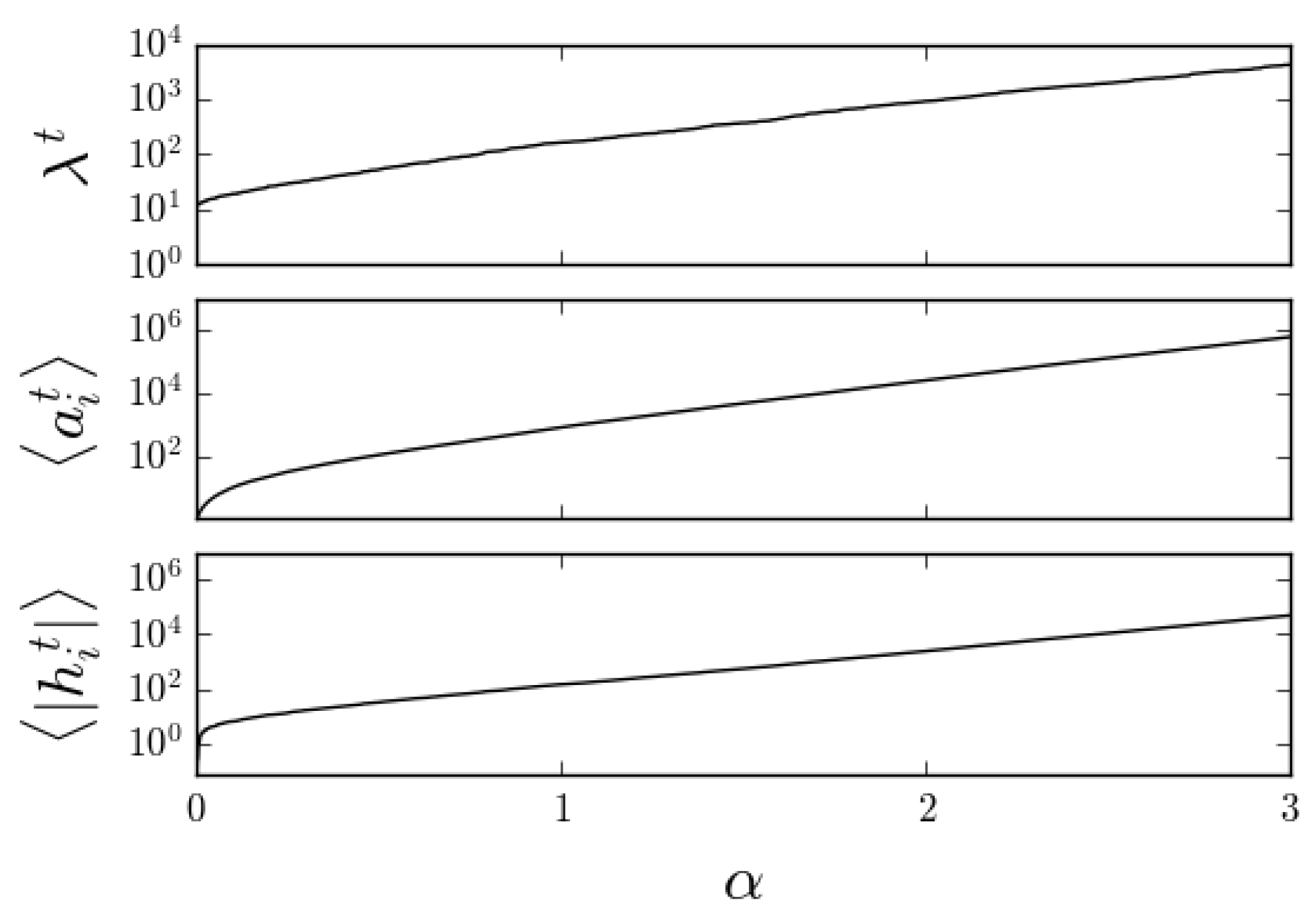
which means that all the natural parameters typically grow with more and more measurements. Similarly, whenever is different from zero, any parameters exhibit a growth in absolute value lead by the factor. For any fixed , these considerations mean that the regularizing effect of the prior in Label (14) would vanish asymptotically in what would be a typical case of a prior being dominated by the likelihood. It is noteworthy that the introduction of a step for the minimization of the KL-divergence in the Bayesian online algorithm results in estimates that typically increase with as well, in a scale similar to the other natural parameters (Figure 5).
6. Conclusions
In this paper, we proposed an online algorithm for Compressed Sensing. Based on an earlier version that expected exact knowledge of the signal generating distribution [24], the present adaptation made use of a double-exponential prior (12) to get rid of this limitation. In order to keep the signal sparsity always in focus during the signal reconstruction, we introduced in this work an extra step where an optimal value for the sparsity-inducing parameter can be estimated as a function of (i.e., a function of the data ). This was achieved through minimization of the KL-divergence between and the (unavailable) full posterior distribution (2), which is approximated by the signal estimate at the previous step.
It is clear that the method is strongly dependent on the validity of the mean-field approximation (6) for the posterior to obtain good reconstruction accuracy. This approximation was introduced in order to simplify the calculations of the moments and to reduce the number of parameters, which should be updated at every step (and, as a consequence, to reduce computational effort and memory requirements). Nevertheless, it is not essential and can be easily replaced by a full Gaussian distribution if needed. In all examples shown here, which made use of signals with fully independent components, the algorithm was shown to give accurate predictions for different signal generating distributions, with and without the presence of additive measurement noise.
Acknowledgments
Paulo V. Rossi would like to thank Yoshiyuki Kabashima for all the discussions that originated this work and Yoshiyuki Kabashima, Andre Manoel and Rafael Calsaverini for all the talks during its production. Renato Vicente would like to thank Julio Stern for many insightful interactions and Paulo V. Rossi and Renato Vicente would like to thank the reviewers for their constructive feedback. This work was partially funded by FAPESP 2014/00792-7 (Paulo V. Rossi). Renato Vicente and Paulo V. Rossi acknowledge the Experian Latam DataLab for supporting this work.
Author Contributions
Paulo V. Rossi and Renato Vicente conceived the algorithm; Paulo V. Rossi performed the simulations; Paulo V. Rossi and Renato Vicente wrote the paper. Both authors have read and approved the final manuscript.
Conflicts of Interest
The authors declare no conflict of interest.
References
- Strohmer, T. Measure What Should be Measured: Progress and Challenges in Compressive Sensing. IEEE Signal Process. Lett. 2012, 19, 887–893. [Google Scholar] [CrossRef]
- Candès, E.J.; Wakin, M.B. An Introduction to Compressive Sampling. IEEE Signal Process. Mag. 2008, 25, 21–30. [Google Scholar] [CrossRef]
- Holtz, O. Compressive sensing: A paradigm shift in signal processing. arXiv, 2008; arXiv:0812.3137. [Google Scholar]
- Donoho, D.L. Compressed sensing. IEEE Trans. Inf. Theory 2006, 52, 1289–1306. [Google Scholar] [CrossRef]
- Eldar, Y.C.; Kutyniok, G. Compressed Sensing: Theory and Applications; Cambridge University Press: Cambridge, UK, 2012. [Google Scholar]
- Nyquist, H. Certain topics in telegraph transmission theory. Trans. AIEE 1928, 47, 617–644. [Google Scholar] [CrossRef]
- Shannon, C. Communication in the presence of noise. Proc. Inst. Radio Eng. 1949, 37, 10–21. [Google Scholar] [CrossRef]
- Candès, E.; Tao, T. Near Optimal Signal Recovery from Random Projections: Universal Encoding Strategies? IEEE Trans. Inf. Theory 2006, 52, 5406–5425. [Google Scholar] [CrossRef]
- Candès, E.J.; Romberg, J.; Tao, T. Robust Uncertainty Principles: Exact Signal Reconstruction from Highly Incomplete Frequency Information. IEEE Trans. Inf. Theory 2006, 52, 489–509. [Google Scholar] [CrossRef]
- Rangan, S. Generalized approximate message passing for estimation with random linear mixing. In Proceedings of the 2011 IEEE International Symposium on Information Theory Proceedings (ISIT), St. Petersburg, Russia, 31 July–5 August 2011. [Google Scholar]
- Krzakala, F.; Mezard, M.; Sausset, F.; Zdeborova, L. Statistical-Physics-Based Reconstruction in Compressed Sensing. Phys. Rev. X 2012, 2, 021005. [Google Scholar] [CrossRef]
- Tramel, E.W.; Manoel, A.; Caltagirone, F.; Gabrié, M.; Krzakala, F. Inferring sparsity: Compressed sensing using generalized restricted Boltzmann machines. In Proceedings of the 2016 IEEE Information Theory Workshop (ITW), Cambridge, UK, 11–14 September 2016; pp. 265–269. [Google Scholar]
- Krzakala, F.; Mezard, M.; Sausset, F.; Sun, Y.; Zdeborova, L. Probabilistic reconstruction in compressed sensing: Algorithms, phase diagrams, and threshold achieving matrices. J. Stat. Mech. Theory Exp. 2012, P08009. [Google Scholar] [CrossRef]
- Xu, Y.; Kabashima, Y.; Zdeborova, L. Bayesian signal reconstruction for 1-bit Compressed Sensing. J. Stat. Mech. Theory Exp. 2014. [Google Scholar] [CrossRef]
- Rangan, S.; Fletcher, A.K.; Goyal, V.K. Asymptotic Analysis of MAP Estimation via the Replica Method and Applications to Compressed Sensing. IEEE Trans. Inf. Theory 2012, 58, 1902–1923. [Google Scholar] [CrossRef] [Green Version]
- Opper, M.; Winther, O. Chapter A Bayesian approach to on-line learning. In On-Line Learning in Neural Networks; Cambridge University Press: Cambridge, UK, 1998; pp. 363–378. [Google Scholar]
- De Oliveira, E.A.; Caticha, N. Inference from aging information. IEEE Trans. Neural Netw. 2010, 21, 1015–1020. [Google Scholar] [CrossRef] [PubMed]
- Vicente, R.; Kinouchi, O.; Caticha, N. Statistical mechanics of online learning of drifting concepts: A variational approach. Mach. Learn. 1998, 32, 179–201. [Google Scholar] [CrossRef]
- Kalman, R.E. A new approach to linear filtering and prediction problems. J. Basic Eng. 1960, 82, 35–45. [Google Scholar] [CrossRef]
- Stengel, R.F. Optimal Control and Estimation; Courier Corporation: North Chelmsford, MA, USA, 2012. [Google Scholar]
- Särkkä, S. Bayesian Filtering and Smoothing; Cambridge University Press: Cambridge, UK, 2013; Volume 3. [Google Scholar]
- Broderick, T.; Boyd, N.; Wibisono, A.; Wilson, A.C.; Jordan, M.I. Streaming variational bayes. In Advances in Neural Information Processing Systems; Curran: Red Hook, NY, USA, 2013; pp. 1727–1735. [Google Scholar]
- Manoel, A.; Krzakala, F.; Tramel, E.W.; Zdeborová, L. Streaming Bayesian inference: Theoretical limits and mini-batch approximate message-passing. arXiv, 2017; arXiv:1706.00705. [Google Scholar]
- Rossi, P.V.; Kabashima, Y.; Inoue, J. Bayesian online compressed sensing. Phys. Rev. E 2016, 94, 022137. [Google Scholar] [CrossRef] [PubMed]
- Tibshirani, R. Regression Shrinkage and Selection via the Lasso. J. R. Stat. Soc. Ser. B (Methodological) 1996, 58, 267–288. [Google Scholar]
- Ganguli, S.; Sompolinsky, H. Statistical Mechanics of Compressed Sensing. Phys. Rev. Lett. 2010, 104, 188701. [Google Scholar] [CrossRef] [PubMed]
- Kabashima, Y.; Wadayama, T.; Tanaka, T. A typical reconstruction limit for compressed sensing based on Lp-norm minimization. J. Stat. Mech. Theory Exp. 2009, 9, L09003. [Google Scholar]
- Baron, D.; Sarvotham, S.; Baraniuk, R.G. Bayesian Compressive Sensing Via Belief Propagation. IEEE Trans. Signal Process. 2010, 58, 269–280. [Google Scholar] [CrossRef]
- Hans, C. Bayesian lasso regression. Biometrika 2009, 96, 835–845. [Google Scholar] [CrossRef]
- Park, T.; Casella, G. The bayesian lasso. J. Am. Stat. Assoc. 2008, 103, 681–686. [Google Scholar] [CrossRef]
- Figueiredo, M.A. Adaptive sparseness for supervised learning. IEEE Trans. Pattern Anal. Mach. Intell. 2003, 25, 1150–1159. [Google Scholar] [CrossRef]
- Efron, B.; Hastie, T.; Johnstone, I.; Tibshirani, R. Least angle regression. Ann. Stat. 2004, 32, 407–499. [Google Scholar]
- Barber, D. Bayesian Reasoning and Machine Learning; Cambridge University Press: Cambridge, UK, 2012. [Google Scholar]
Figure 1.
Schematic representation of the measurement process in Compressed Sensing. The sparse signal is projected onto a (known) random measurement vector . The result goes through a channel giving rise to the value .
Figure 1.
Schematic representation of the measurement process in Compressed Sensing. The sparse signal is projected onto a (known) random measurement vector . The result goes through a channel giving rise to the value .

Figure 2.
Update and projection steps.

Figure 3.
L1-based reconstruction for CS with for signals generated by . (a) and (b): ; (c) and (d): . The top row consists of the noiseless standard CS scenario; the bottom row corresponds to the noisy scenario with . In all figures, dashed lines were obtained with known and full lines with estimated through (19). In (a), the average error of 100 simulations each of and 2000 for chosen values of are shown as crosses (unknown ) and triangles (known ). The error decreases with increasing N. All lines in all pictures then correspond to the extrapolation of these finite N values to by means of a quadratic fit. All pictures: .

Figure 4.
Difference between (from Label (6), where the exact prior is considered) and the true signal sparsity . The full line corresponds to the average of 100 simulations of the noisy standard CS scenario with , , and . The dashed line is the true sparsity of the original signal . Inset: Mean variance. Notice that the absolute value approximation gets progressively better with growing . Indeed, its accuracy matches the diminishing of the posterior distribution’s variance.
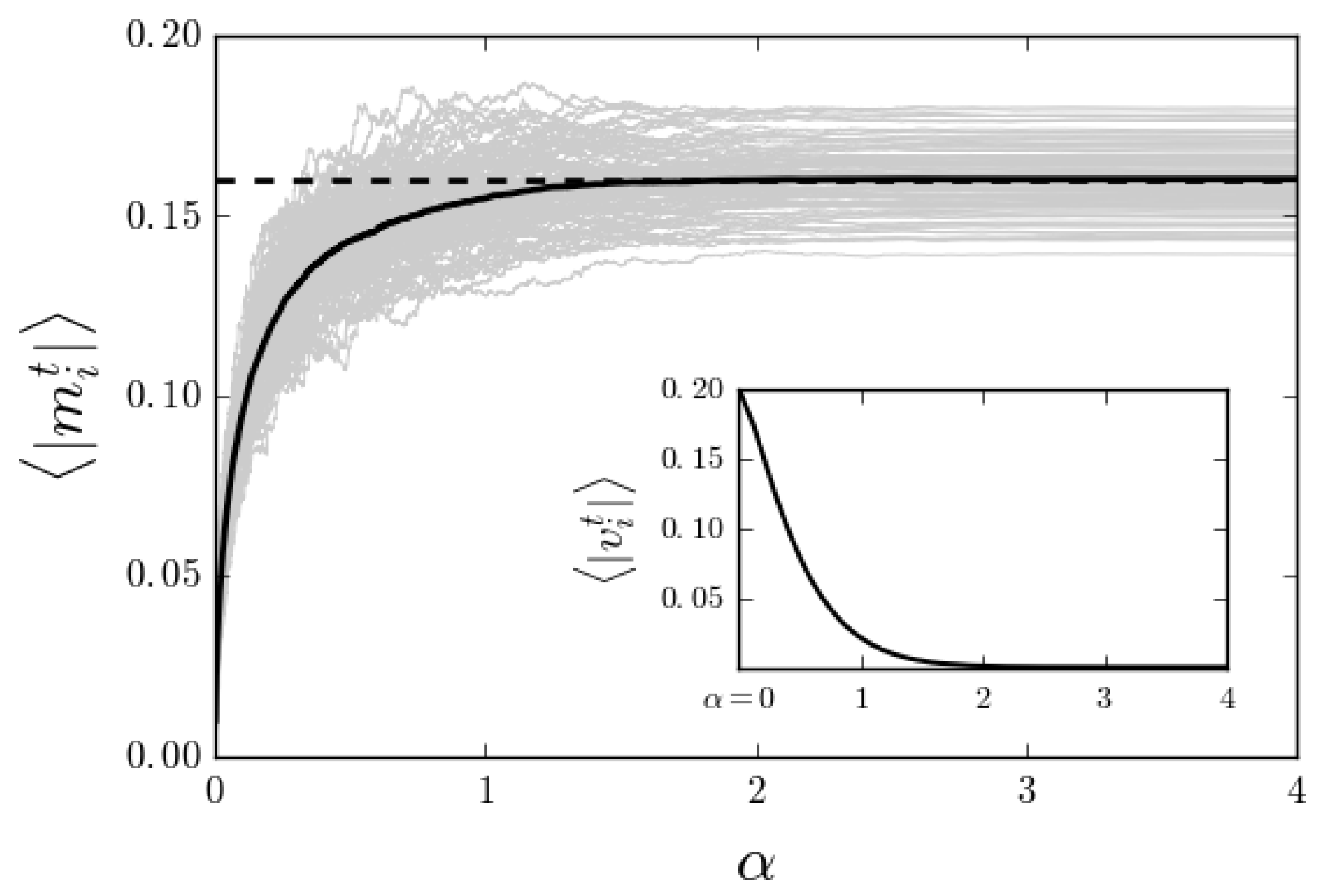
Figure 5.
An example of the online CS algorithm where has been adjusted after all measurements so that the inferred signal sparsity was equal to the known value . Note that , just like the natural parameters , typically grows exponentially. Here, , , and .
Figure 5.
An example of the online CS algorithm where has been adjusted after all measurements so that the inferred signal sparsity was equal to the known value . Note that , just like the natural parameters , typically grows exponentially. Here, , , and .

© 2017 by the authors. Licensee MDPI, Basel, Switzerland. This article is an open access article distributed under the terms and conditions of the Creative Commons Attribution (CC BY) license (http://creativecommons.org/licenses/by/4.0/).
Share and Cite
MDPI and ACS Style
Rossi, P.V.; Vicente, R. L1-Minimization Algorithm for Bayesian Online Compressed Sensing. Entropy 2017, 19, 667. https://doi.org/10.3390/e19120667
AMA Style
Rossi PV, Vicente R. L1-Minimization Algorithm for Bayesian Online Compressed Sensing. Entropy. 2017; 19(12):667. https://doi.org/10.3390/e19120667
Chicago/Turabian StyleRossi, Paulo V., and Renato Vicente. 2017. "L1-Minimization Algorithm for Bayesian Online Compressed Sensing" Entropy 19, no. 12: 667. https://doi.org/10.3390/e19120667
Note that from the first issue of 2016, this journal uses article numbers instead of page numbers. See further details here.