A Geodesic-Based Riemannian Gradient Approach to Averaging on the Lorentz Group

1
School of Mathematics and Statistics, Beijing Institute of Technology, Beijing 100081, China
2
Beijing Key Laboratory on MCAACI, Beijing Institute of Technology, Beijing 100081, China
3
Department of Mathematics, Duke University, Durham, NC 27708, USA
*
Author to whom correspondence should be addressed.
Entropy 2017, 19(12), 698; https://doi.org/10.3390/e19120698
Submission received: 19 November 2017
/
Revised: 16 December 2017
/
Accepted: 17 December 2017
/
Published: 20 December 2017
(This article belongs to the Special Issue Entropic Aspects Arising from Geometric Descriptions of Physical Phenomena)
Abstract
:In this paper, we propose an efficient algorithm to solve the averaging problem on the Lorentz group . Firstly, we introduce the geometric structures of endowed with a Riemannian metric where geodesic could be written in closed form. Then, the algorithm is presented based on the Riemannian-steepest-descent approach. Finally, we compare the above algorithm with the Euclidean gradient algorithm and the extended Hamiltonian algorithm. Numerical experiments show that the geodesic-based Riemannian-steepest-descent algorithm performs the best in terms of the convergence rate.
1. Introduction
Averaging measured data on matrix manifolds is one of the most frequently arising problems in many fields. For example, one may need to determine an average eye of a set of optical systems [1]. In [2], the authors concern the statistics of covariance matrices for biomedical engineering applications. The current research mainly focuses on the compact Lie groups, such as the special orthogonal group [3] and the unitary group [4], or other matrix manifolds, such as the special Euclidean group [5], Grassmann manifold [6,7], the Stiefel manifold [8,9] and the symmetry positive-definite matrix manifold [10,11]. However, there is little research on averaging over the Lorentz group .
In [12], Clifford algebra, as a generalization of quaternions, is applied to approximate the average on the special Lorentz group . In engineering, the Lorentz group plays a fundamental role, e.g., in the analysis of motion of charged particles in electromagnetism [13]. In physics, the Lorentz group forms a basis for the transformation of parabolic catadioptric image features [14]. According to [15], the Lorentz group is equal to the linear transformations of the projective plane and used to characterize the catadioptric fundamental matrices that are applied to study the catadioptric cameras.
This paper aims at investigating the averaging on the Lorentz group with a left-invariant metric that plays the role of Riemannian metric so that the geodesic is given in closed form. The considered averaging optimization problem could be solved numerically via a geodesic-based Riemannian-steepest-descent algorithm (RSDA). Furthermore, the devised method RSDA is compared with the line-search algorithm, Euclidean gradient algorithm (EGA) and the second-order learning algorithm, extended Hamiltonian algorithm (EHA), proposed in [16,17].
The remainder of the paper is organized as follows. In Section 2, we summarize the geometric structures of the Lorentz group. The averaging optimization problem, the geodesic-based Riemannian-steepest-descent algorithm and the extended Hamiltonian algorithm on the Lorentz group are presented in Section 3. In Section 4, we show the numerical results of the RSDA and compare the convergence rate of the RSDA with the other two algorithms. Section 5 presents the conclusions of the paper.
2. Geometry of the Lorentz Group
In this section, we review the foundations of Lorentz group and describe a Riemannian metrization in which the geodesic could be written in closed forms.
Let be the set of real matrices and be its subset containing only nonsingular matrices. It is well-known that is a Lie group, i.e., a group which is also a differentiable manifold and for which the operations of group multiplication and inverse are smooth.
Definition 1.
The Lorentz group as a Lie subgroup of is defined by
where I is identity matrix, and is zero matrix.
For any , the following identities hold:
The tangent space , the Lie algebra and the normal space associated with the Lorentz group can be characterized as follows:
We employ the left-invariant metric as the Riemannian metric on at
Let be a smooth curve in , and its length associated with the Riemannian metric (1) is defined as
The geodesic distance between two points and in is the infimum of lengths of curves connecting them, namely,
Applying the variational method from Equation (2), we can find that the geodesic equation satisfies
where denotes the Christoffel symbol, the over-dot and the double over-dot denote first-order and second-order derivation with respect to parameter t, respectively. When the values and are specified, we shall denote the solution as , which is associated with the Riemannian exponential map defined as
Let be a differentiable function and denotes the Riemannian gradient of function f with respect to the metric (1), which is defined by the compatibility condition
where denotes the Euclidean gradient of function f and denotes the Euclidean metric.
The exponential of a matrix A in is defined by
We remark that when for A and B in .
For the Frobenius norm , when , the logarithm of A is given by
In general, . We here recall the important fact that
Lemma 1.
Suppose that is a scalar function of matrix A in [18]. If
holds, then
where denotes the derivative of .
The structure of the Riemannian gradient associated with the Riemannian metric (1) is given by the following result.
Theorem 1.
The Riemannian gradient of a sufficiently regular function associated with the Riemannian metric (1) satisfies
Proof of Theorem 1.
According to equality (3), the gradient is computed as
as X is arbitrary, the condition above implies that , hence , with , and thus we have
Since , we have
Inserting the expression into the equation above, we have
Substituting S into the expression of , we finish the proof. ☐
In the text, we would like to give credit to [19] for the explicit expression of geodesic over the general linear group endowed with the natural left-invariant Riemannian metric (1). Under the same Riemannian metric, it is clear that the geodesic on the Lorentz group can be written in closed form (cf. Theorem 2.14 in [19]).
Proposition 1.
The geodesic , with , corresponding to the Riemannian metric (1) has expression
Proof of Proposition 1.
In fact, by the variational formula , the geodesic equation in Christoffel form reads
By the definition that , we see that the geodesic satisfies the Euler–Lagrange equation
We can verify that the curve emanating from A with a velocity X is the solution of the Euler–Lagrange equation above. ☐
Remark 1.
From the proof of Proposition 1 and the fact , , we conclude that
3. Optimization on the Lorentz Group
This section aims at investigating the averaging optimization problem on the Lorentz group, and finding the average value out of a set of Lorentz matrices. Section 3.1 and Section 3.2 recall the geodesic-based Riemannian-steepest-descent algorithm and the extended Hamiltonian algorithm on the Lorentz group, respectively.
3.1. Riemannian-Steepest-Descent Algorithm on the Lorentz Group
Note that the geodesic distance . From Equation (6), it is difficult to give an explicit expression of X in A and B. In [20], the authors show that the geodesic distance connecting A and B could be obtained by solving the following problem
Then, the geodesic distance between A and B, , where is a minimizer of Equation (8). In order to compute , a descent procedure can be applied so we need to find the gradient first. The differential with respect to U of the function is given by
and thus, according to Lemma 1, we can get the Euclidean gradient of
On the other hand, recall the Goldberg exponential formula in [21]
where denotes a word in the letters X and Y, and the inner sum is over all words with length . The symbol denotes Goldberg coefficient on the word , a rational number. If the word begins with X, say
where are positive integers satisfying , and denotes if m is odd and if m is even. is similarly defined.
The Goldberg coefficient is
in which and , denotes the greatest integer of the enclosed number, and the polynomials are defined recursively by and for .
According to Theorem 1 in [22], we can obtain the following result.
Proposition 2.
If , then
Proof of Proposition 2.
According to the Goldberg exponential formula (10), Equation (7) can be recast as
in which denotes a word in the letters and .
By using properties of the Goldberg coefficient (see [23]), we get
where is the usual binomial coefficient. Furthermore, the number of words of length is just . Thus, the sum of extended over all words of length n and involved m parts is
Therefore, due to , and for , , we have
Here, in the last step, the equality holds if and only if . ☐
Remark 2.
If the condition , is added, then, when ,
Remark 3.
Proposition 2 implies that we can replace the geodesic distance by where the latter one is much easier to handle.
In order to compare different Lorentz matrices, the following discrepancy is defined
For the Lorentz group, the criterion function to measure a collection of samples randomly generated is defined by
which appears as a specialization, to the Lorentz group, of the Karcher criterion [24].
Definition 2.
The average value of is defined as
Based on the case in the Euclidean space of the line search method with the negative Euclidean gradient, in order to achieve the average value, a geodesic-based Riemannian-steepest-descent algorithm can be expressed as [25]
where is an iteration step-counter, the initial guess is arbitrarily chosen, and denotes a (possibly variable) stepsize schedule.
Note that the Riemannian gradient of the criterion function is crucial to solving the optimization problem by the geodesic-based Riemannian-steepest-descent algorithm (16).
Theorem 2.
The Riemannian gradient of the criterion function (14) is
Proof of Theorem 2.
The differential with respect to A of the criterion function (14) is
and, furthermore, according to Lemma 1, we get the Euclidean gradient
Associated with the expressions of the geodesic (5) and the Riemannian gradient (17) of the criterion function, the geodesic-based Riemannian-steepest-descent algorithm (16) is recast as
where .
In order to compute a nearly-optimal stepsize, the function considered as a function of the stepsize can be expanded in Taylor series at the point as
where the and as the coefficients of the Taylor expansion are computed by
Furthermore, the nearly-optimal stepsize value that minimizes the is provided that , , hence .
Thus, to obtain the and , the function is recast as
Calculation leads to the first-order derivative of the function
and setting yields the
Under the first-order derivative of the function above, direct calculations lead to the second-order derivative of the function
and, setting we get
Hence, the nearly-optimal stepsize of the geodesic-based Riemannian-steepest-descent algorithm (19) is
3.2. Extended Hamiltonian Algorithm on the Lorentz Group
References [16,17] introduced a general theory of extended Hamiltonian (second order) learning on Riemannian manifold, especially, as an instance of learning by constrained criterion function optimization on the matrix manifolds. For the Lorentz group, the extended Hamiltonian algorithm can be expressed by
where , denotes the instantaneous learning velocity, denotes a criterion function, and the constant denotes a viscosity parameter.
Inserting the the expressions of the Christoffel matrix function in Remark 1 and the Riemannian gradient (4) into the general extended Hamiltonian system (22), calculations lead to the following expressions:
Hence, the second equation may be integrated numerically by a Euler stepping method, while the first one may be integrated via the geodesic. Namely, system (22) may be implemented by
where denotes the learning rate. The effectiveness of the algorithm is ensured if and only if
where denotes the largest eigenvalue of the Hessian matrix of the criterion function (see [17]).
4. Numerical Experiments
In the present section, we give two numerical experiments on the Lorentz group to demonstrate the effectiveness and performance of the proposed algorithms. The Lorentz group as a homogeneous space has four connected components. Now, we study the optimization on a connected component containing the identical matrix .
In order to emphasize the behavior of the optimization methods RSDA, the EHA and the EGA, in the following experiments, and are used.
4.1. Numerical Experiments on Averaging Two Lorentz Matrices
In Section 3.1, it is noticed that the geodesic distance and the discrepancy between two points A and B are different. Now, given , , numerical experiment results are shown to compare and . The following two points are sought:
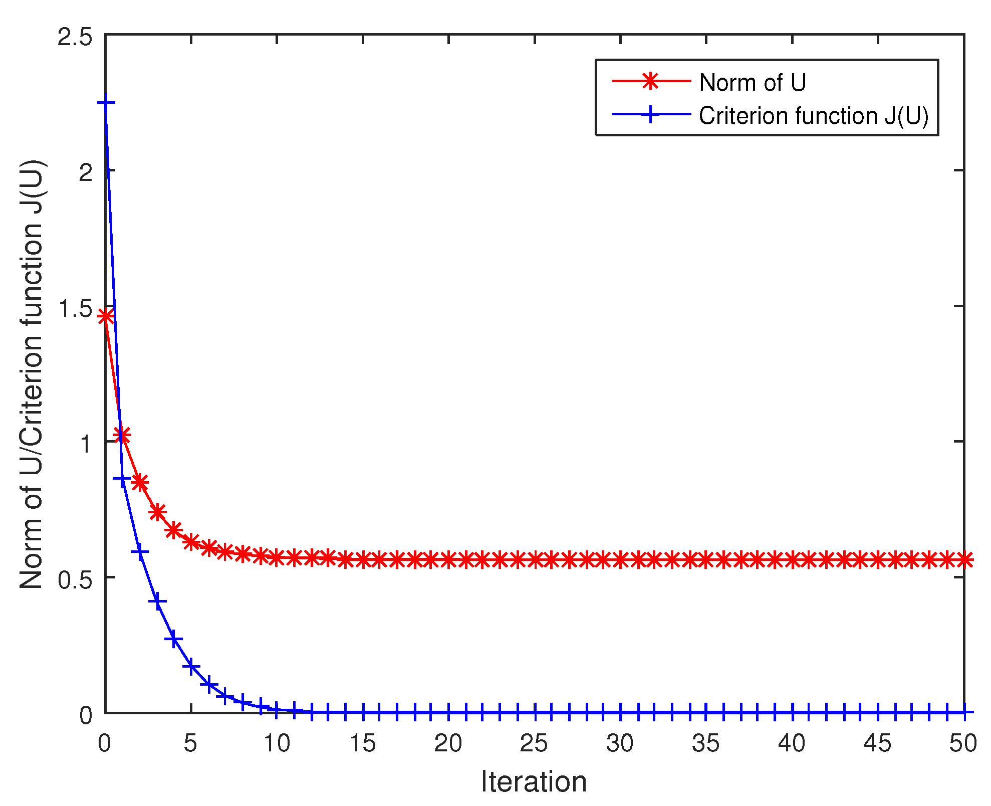
It can be verified that , , . The optimization problem to compute the geodesic distance can be solved by means of a descent procedure along the negative Euclidean gradient (9) with a line search strategy. In Figure 1, the results show that the Frobenius norm of U is decreasing steadily when the criterion function tends to be constant 0 during iteration. By the numerical experiments, we can get
It is interesting that the geodesic distance between and is , and the discrepancy between and is .
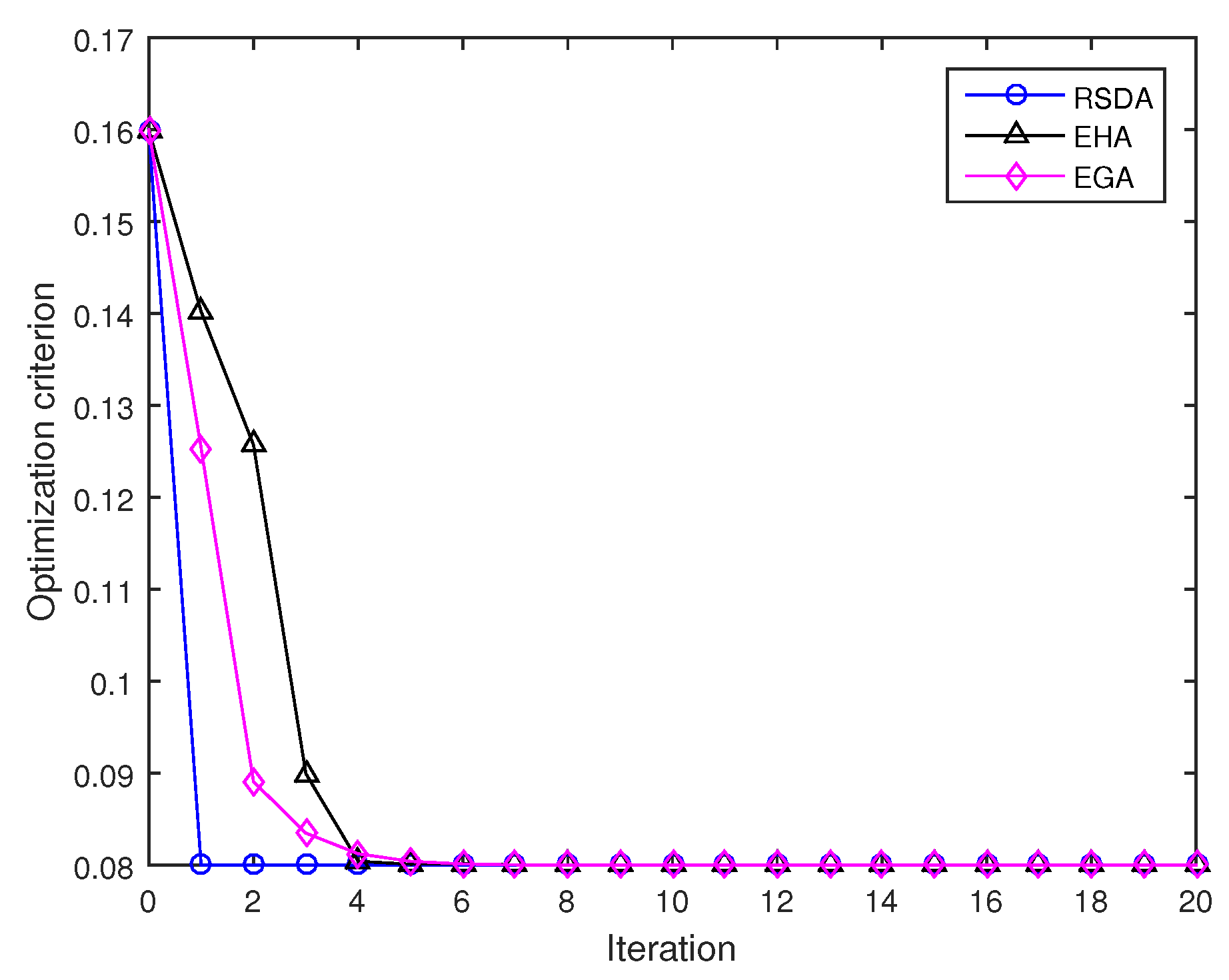
In the following experiment, we consider the average value of two points and . Figure 2 displays the results of running the RSDA, the EHA, and the EGA. Note that the iteration sequence is expected to converge to a matrix that locates amid the samples , and the condition holds. The initial point is set as , which satisfies . More initial points can be chosen in a neighbor of the matrix by the following rule (25). It can be found that the averaging algorithms converge steadily and the RSDA has the fastest convergence rate among three algorithms and needs one iteration to obtain the average value as follows:
However, the EHA and the EGA need 13 and 18 iterations to realize the same accuracy, respectively. It is interesting to compare the discrepancy with the discrepancy , which confirms that the computed average value is truly a midpoint (i.e., it is located at approximately equal discrepancy from the two matrices).
4.2. Numerical Experiments on Averaging Several Lorentz Matrices
The numerical experiments rely on the availability of a way to generate pseudo-random samples on the Lorentz group. Given a point which is referred to as “center of mass” or simply center of the random distribution, it is possible to generate a random sample in a neighbor of a matrix B by the rule [26,27]
where the center matrix B can be generated by a curve departing from the identical matrix, with V generated randomly matrix in .
According to the structure of the tangent space , expression (24) can be written
where is any unstructured random matrix.
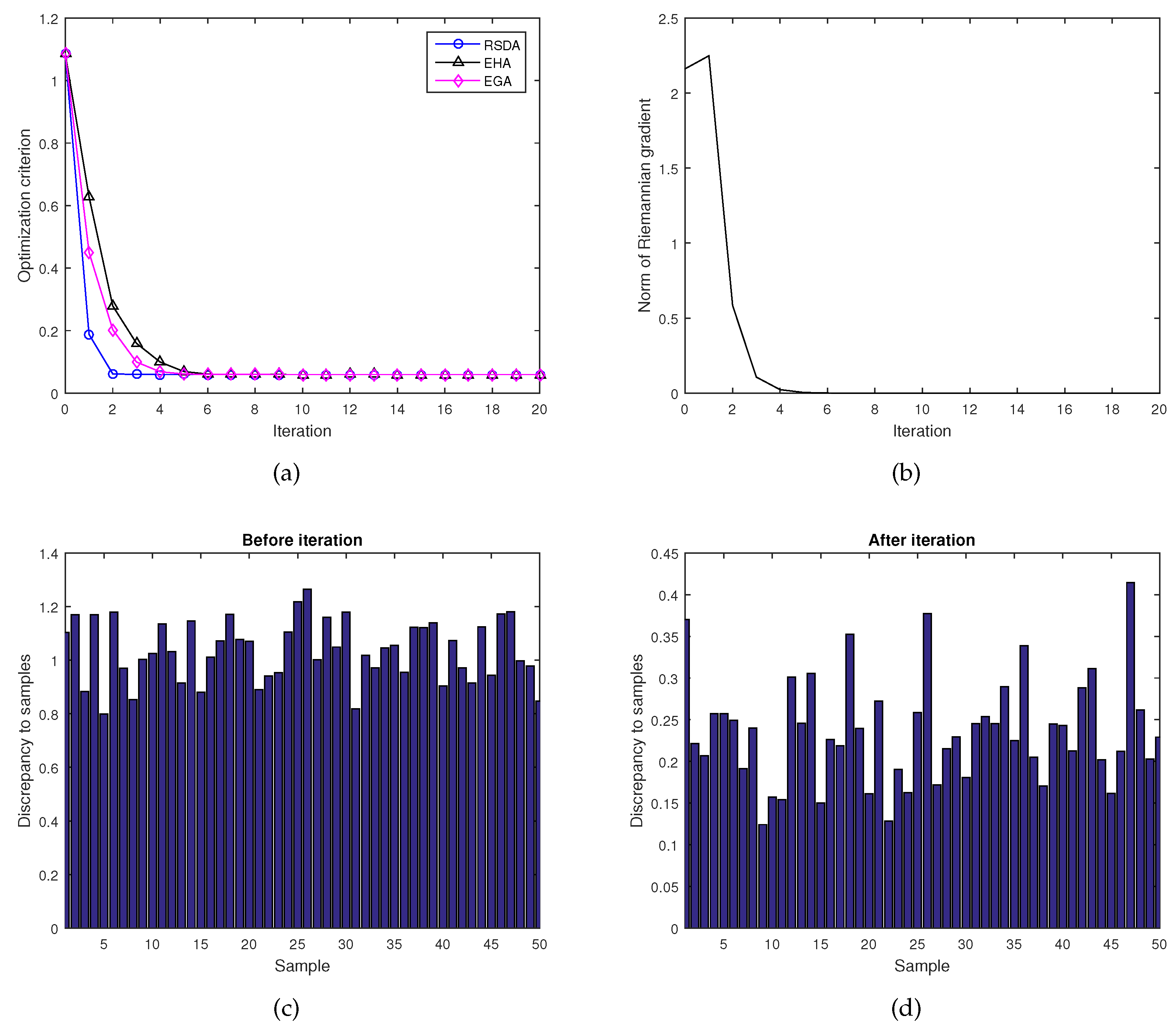
Figure 3 displays the results on optimization over with N = 50 Lorentz matrices. The initial point is randomly generated,
Figure 3a shows the values of the criterion function (14) through the RSDA, the EHA and the EGA. Numerical experiments show that the average value of 50 Lorentz matrices is
which can be obtained after seven iterations using the RSDA, while the EHA and the EGA need 15 iterations. Figure 3b gives the norm of the Riemannian gradient (17) during iteration by the RSDA, from which we can obtain that the norm of the Riemannian gradient tends to be constant 0 after iteration 6. Figure 3c,d give the values of the discrepancy before iteration and after iteration, respectively. In particular, note that all the discrepancy from the samples and the matrix A are decreased substantially. The results show that the convergence rate of the RSDA is still the fastest among three algorithms.
5. Conclusions
In this paper, we consider the averaging optimization problem for the Lorentz group , namely, to measure the average of a set of Lorentz matrices. In order to tackle the related optimization problem, a geodesic-based Riemannian-steepest-descent algorithm is presented on the Lorentz group endowed with a left-invariant metric (Riemannian metric). The devised averaging algorithm is compared with the extended Hamiltonian algorithm and the Euclidean gradient algorithm. The results of numerical experiments over the Lorentz group show that the convergence rate of the geodesic-based Riemannian-steepest-descent algorithm is the best one among these three algorithms.
Acknowledgments
The present research is supported by the National Natural Science Foundations of China (No. 61179031).
Author Contributions
Jing Wang conceived and designed the experiments; Jing Wang performed the experiments; Jing Wang and Huafei Sun analyzed the data; Didong Li contributed reagents/materials/analysis tools; Jing Wang, Huafei Sun and Didong Li wrote the paper.
Conflicts of Interest
The authors declare no conflict of interest.
References
- Harris, W.F. Paraxial ray tracing through noncoaxial astigmatic optical systems, and a 5 × 5 augmented system matrix. Optom. Vis. Sci. 1994, 71, 282–285. [Google Scholar] [CrossRef] [PubMed]
- Barachant, A.; Bonnet, S.; Congedo, M.; Jutten, C. Multi-class brain computer interface classification by Riemannian geometry. IEEE Trans. Bio. Med. Eng. 2012, 59, 920–928. [Google Scholar] [CrossRef] [PubMed] [Green Version]
- Moakher, M. Means and averaging in the group of rotations. SIAM J. Matrix Anal. A 2002, 24, 1–16. [Google Scholar] [CrossRef]
- Mello, P.A. Averages on the unitary group and applications to the problem of disordered conductors. J. Phys. A 1990, 23, 4061–4080. [Google Scholar] [CrossRef]
- Duan, X.M.; Sun, H.F.; Peng, L.Y. Riemannian means on special Euclidean group and unipotent matrices group. Sci. World J. 2013, 2013, 292787. [Google Scholar] [CrossRef] [PubMed]
- Chakraborty, R.; Vemuri, B.C. Recursive Fréchet mean computation on the Grassmannian and its applications to computer vision. In Proceedings of the IEEE International Conference on Computer Vision (ICCV), Santiago, Chile, 7–13 December 2015. [Google Scholar]
- Fiori, S.; Kaneko, T.; Tanaka, T. Tangent-bundle maps on the Grassmann manifold: Application to empirical arithmetic averaging. IEEE Trans. Signal Process. 2015, 63, 155–168. [Google Scholar] [CrossRef]
- Kaneko, T.; Fiori, S.; Tanaka, T. Empirical arithmetic averaging over the compact Stiefel manifold. IEEE Trans. Signal Process. 2013, 61, 883–894. [Google Scholar] [CrossRef]
- Pölitz, C.; Duivesteijn, W.; Morik, K. Interpretable domain adaptation via optimization over the Stiefel manifold. Mach. Learn. 2016, 104, 315–336. [Google Scholar] [CrossRef]
- Fiori, S. Learning the Fréchet mean over the manifold of symmetric positive-definite matrices. Cogn. Comput. 2009, 1, 279–291. [Google Scholar] [CrossRef]
- Moakher, M. A differential geometric approach to the geometric mean of symmetric positive-definite matrices. SIAM J. Matrix Anal. A 2005, 26, 735–747. [Google Scholar] [CrossRef]
- Buchholz, S.; Sommer, G. On averaging in Clifford groups. In Computer Algebra and Geometric Algebra with Applications; Springer: Berlin/Heidelberg, Germany, 2005; Volume 3519, pp. 229–238. [Google Scholar]
- Kawaguchi, H. Evaluation of the Lorentz group Lie algebra map using the Baker-Cambell-Hausdorff formula. IEEE Trans. Magn. 1999, 35, 1490–1493. [Google Scholar] [CrossRef]
- Heine, V. Group Theory in Quantum Mechanics; Dover: New York, NY, USA, 1993. [Google Scholar]
- Geyer, C.M. Catadioptric Projective Geometry: Theory and Applications. Ph.D. Thesis, University of Pennsylvania, Philadelphia, PA, USA, 2002. [Google Scholar]
- Fiori, S. Extended Hamiltonian learning on Riemannian manifolds: Theoretical aspects. IEEE Trans. Neural Netw. 2011, 22, 687–700. [Google Scholar] [CrossRef] [PubMed]
- Fiori, S. Extended Hamiltonian learning on Riemannian manifolds: Numerical aspects. IEEE Trans. Neural Netw. Learn. Syst. 2012, 23, 7–21. [Google Scholar] [CrossRef] [PubMed]
- Zhang, X. Matrix Analysis and Application; Springer: Beijing, China, 2004. [Google Scholar]
- Andruchow, E.; Larotonda, G.; Recht, L.; Varela, A. The left invariant metric in the general linear group. J. Geom. Phys. 2014, 86, 241–257. [Google Scholar] [CrossRef]
- Zacur, E.; Bossa, M.; Olmos, S. Multivariate tensor-based morphometry with a right-invariant Riemannian distance on GL+(n). J. Math. Imaging Vis. 2014, 50, 19–31. [Google Scholar] [CrossRef]
- Goldberg, K. The formal power series for log(exey). Duke Math. J. 1956, 23, 1–21. [Google Scholar] [CrossRef]
- Newman, M.; So, W.; Thompson, R.C. Convergence domains for the Campbell-Baker-Hausdorff formula. Linear Algebra Appl. 1989, 24, 30–310. [Google Scholar] [CrossRef]
- Thompson, R.C. Convergence proof for Goldberg’s expoential series. Linear Algebra Appl. 1989, 121, 3–7. [Google Scholar] [CrossRef]
- Karcher, H. Riemannian center of mass and mollifier smoothing. Commun. Pure Appl. Math. 1977, 30, 509–541. [Google Scholar] [CrossRef]
- Gabay, D. Minimizing a differentiable function over a differentiable manifold. J. Optim. Theory App. 1982, 37, 177–219. [Google Scholar] [CrossRef]
- Fiori, S. Solving minimal-distance problems over the manifold of real symplectic matrices. SIAM J. Matrix Anal. A 2011, 32, 938–968. [Google Scholar] [CrossRef]
- Fiori, S. A Riemannian steepest descent approach over the inhomogeneous symplectic group: Application to the averaging of linear optical systems. Appl. Math. Comput. 2016, 283, 251–264. [Google Scholar] [CrossRef]
Figure 1.
The criterion function and the Frobenius norm of U during iteration, respectively.

Figure 2.
Convergence comparison among the Riemannian-steepest-descent algorithm (RSDA), the extended Hamiltonian algorithm (EHA) and the Euclidean gradient algorithm (EGA) during iteration.
Figure 2.
Convergence comparison among the Riemannian-steepest-descent algorithm (RSDA), the extended Hamiltonian algorithm (EHA) and the Euclidean gradient algorithm (EGA) during iteration.

Figure 3.
(a) convergence comparison among the RSDA, the EHA and the EGA during iteration; (b) the norm of the Riemannian gradient (17) during iteration by the Riemannian-steepest-descent algorithm (RSDA); (c–d) the discrepancy before iteration and after iteration , respectively.
Figure 3.
(a) convergence comparison among the RSDA, the EHA and the EGA during iteration; (b) the norm of the Riemannian gradient (17) during iteration by the Riemannian-steepest-descent algorithm (RSDA); (c–d) the discrepancy before iteration and after iteration , respectively.
© 2017 by the authors. Licensee MDPI, Basel, Switzerland. This article is an open access article distributed under the terms and conditions of the Creative Commons Attribution (CC BY) license (http://creativecommons.org/licenses/by/4.0/).
Share and Cite
MDPI and ACS Style
Wang, J.; Sun, H.; Li, D. A Geodesic-Based Riemannian Gradient Approach to Averaging on the Lorentz Group. Entropy 2017, 19, 698. https://doi.org/10.3390/e19120698
AMA Style
Wang J, Sun H, Li D. A Geodesic-Based Riemannian Gradient Approach to Averaging on the Lorentz Group. Entropy. 2017; 19(12):698. https://doi.org/10.3390/e19120698
Chicago/Turabian StyleWang, Jing, Huafei Sun, and Didong Li. 2017. "A Geodesic-Based Riemannian Gradient Approach to Averaging on the Lorentz Group" Entropy 19, no. 12: 698. https://doi.org/10.3390/e19120698
Note that from the first issue of 2016, this journal uses article numbers instead of page numbers. See further details here.