Research and Application of a Novel Hybrid Model Based on Data Selection and Artificial Intelligence Algorithm for Short Term Load Forecasting

Abstract

Machine learning plays a vital role in several modern economic and industrial fields, and selecting an optimized machine learning method to improve time series’ forecasting accuracy is challenging. Advanced machine learning methods, e.g., the support vector regression (SVR) model, are widely employed in forecasting fields, but the individual SVR pays no attention to the significance of data selection, signal processing and optimization, which cannot always satisfy the requirements of time series forecasting. By preprocessing and analyzing the original time series, in this paper, a hybrid SVR model is developed, considering periodicity, trend and randomness, and combined with data selection, signal processing and an optimization algorithm for short-term load forecasting. Case studies of electricity power data from New South Wales and Singapore are regarded as exemplifications to estimate the performance of the developed novel model. The experimental results demonstrate that the proposed hybrid method is not only robust but also capable of achieving significant improvement compared with the traditional single models and can be an effective and efficient tool for power load forecasting.

1. Introduction

Accurate short-term load forecasting (STLF) plays a vital part in power system operation. A highly accurate forecasting method is one of the most important approaches used in improving power system management, especially in the power market [1]. Effective forecasting helps to establish electrical power scheduling and reduce management risk, which is an absolutely necessary component of power system risk management [2,3]. If the performance of the electric load forecasting model could be effectively boosted, considerable influence would be produced. Taking China as an example, the State Grid Corporation of China has rules stating that the spinning reserve capacity must be 3%–5% of the installed capacity. If the forecasting accuracy could be improved by 1%, a considerable economic benefit would be generated, i.e., approximately 161,042.688 MW h energy in one day and 58,780,581.12 MW h in one year could be saved [4].

In contrast, inaccurate forecast results lead to considerable electrical power system losses. Overestimated forecasts will produce unnecessary electricity; alternately, underestimated forecasts will cause trouble in providing enough electrical power, and that means high losses for the power market [5]. Meanwhile, inaccurate forecasts will lead to a direct increase of operating costs, and the operation of the power system is very sensitive to load forecasting errors. Hobbs et al. [6] concluded that a decrease in power load forecasting error in terms of a mean absolute percentage error of 1% reduces the variable generation cost between $0.6 and $1.6 million annually for a 10,000 MW utility with an MAPE of approximately 4%. Many severe blackout disasters that seriously affected the normal production and lives of people have been documented. Examples include the U.S.–Canada blackout in 2003, the southern part of Moscow blackout in 2005, the New York blackout in 2006 and the Indian power grid collapse in 2012 [7,8]. Obviously, if we could generate an early warning before these events, based on a robust forecasting model, effective measures could be taken to avoid these types of accidents. However, electric power systems are influenced by many factors, including holidays, policy, the social and natural environment, etc. [9]. Therefore, developing a novel and robust load forecasting algorithm and improving the forecasting performance are highly desirable for power load forecasts.

Some researchers began to focus on the short-term load forecasting several years ago; hence, a variety of models have been developed and proposed for STLF. These forecasting algorithms can be classified into two types: conventional statistical algorithms and artificial intelligence algorithms. The conventional statistical algorithms, which are regarded as stochastic time series models, only employ historical data. These algorithms are simple to apply and easy to implement. Therefore, a variety of time series models are commonly employed in load prediction, including the autoregressive model [10], autoregressive moving average model [11,12], autoregressive integrated moving average model [13], regression model [14], multiple linear regression [15], general exponential smoothing [16], Kalman filtering method [17], etc. However, the relevant literature suggests that traditional methods have unavoidable defects, i.e., they cannot effectively interpret the complicated relationship between electric power load data and stochastic factors such as social events and time periodicity; thus, the defects can lead to highly unpredictable variations in power demand [18].

The artificial intelligence models have been widely used in several areas, mainly because of their flexibility, symbolic reasoning and explanation capabilities [19]. Moreover, the artificial intelligence algorithms are recognized as powerful forecasting tools with strong robustness and fault tolerance to solve the STLF problem, influenced by several factors to achieve better performance [20]. Thus, there has been much research work focusing on using the artificial intelligence and new models to improve forecasting accuracy and stability. A hybrid model based on the modified differential evolution algorithm and the wavelet neural network model was employed for electrical load forecasting [21]. Zhao and Guo [22] proposed a novel hybrid optimized gray model to forecast annual power load series. Kelo et al. [18] presented a novel neural network, a combination of the wavelet and Elman network, to predict one-day-ahead power load under the influence of temperature. Hu et al. [23] proposed a hybrid filter–wrapper feature selection method for short-term load forecasting. Xiao et al. developed a combined model based on multiple seasonal patterns and the modified firefly algorithm in [4] and an integrated model based on the multi-objective optimization algorithm in [24] for electrical load forecasting. A novel hybrid model was developed by Niu et al. [25] for short-term load forecasting, which combined singular spectrum analysis, the nonlinear multi-layer perceptron network and the integrated intelligent optimization algorithm.

The SVR model has superiority in fitting high dimensional nonlinear data and has been applied in many areas, such as agricultural commodity future prices forecasting [26], stock price index forecasting [27], air passenger traffic forecasting [28], holiday daily tourist flow forecasting [29], air quality early-warning systems [30], etc. Moreover, in the electricity power forecasting fields, Hong et al. [31,32,33,34] proposed various SVR-based load forecasting models, which included the artificial intelligence algorithm to optimize its parameters, to achieve more accurate forecasting performance. Moreover, Huang [35] developed an SVR-based model that combined the chaotic mapping function and quantum particle swarm optimization algorithm to improve the forecasting accuracy. Lee and Lin [36] proposed an SVR-based model that combines quantum behaviors and the tabu search algorithm with the SVR model for electricity load forecasting. Moreover, De Giorgi et al. [37,38] proposed a series of hybrid photovoltaic power forecasting models, which were based on the least square support vector machine models, to improve the performance of the forecast.

The previous literature review illustrates that the hybrid forecasting model has become a trend. Some drawbacks of the models discussed above can be summarized [39,40]: (1) the traditional statistical models have a high dependence on data, a poor extrapolation effect and narrow forecasting scale, being more suitable for data featured by linear trends and unable to capture data with high fluctuation and noise. More importantly, the data of an electrical power system always features high volatility, irregularity or other tendencies due to the influence of several factors. If the environmental or sociological factors change suddenly, the forecasting errors will increase greatly, which is the worst drawback of statistical models [41]; (2) Artificial neural networks (ANNs) are unstable and have a relative dependence on data, making it difficult to scientifically determine the network structure; furthermore, they can easily fall into a local minimum. Therefore, the SVR model and optimization algorithms are employed to overcome the drawbacks of ANNs; (3) The single models never pay attention to the significance of data selection, signal processing and optimization, and hence cannot always satisfy the requirements of time series forecasting; (4) The one-step forecasting accuracy is higher, while the multi-step forecasting always has a lower accuracy or unreliable results. Therefore, based on the limitations discussed above, and with the current tendency of the hybrid model being considered as the mainstream, a hybrid SVR-based forecasting model is developed; it successfully overcomes these drawbacks, considering periodicity, trend and randomness for electrical load time series. More specifically, the SVR model, acknowledged as one of the top ten models in data mining, is adopted as the basic forecasting model to develop a robust model for short-term load forecasting in this paper. To further improve the forecasting performance, an innovative hybrid forecasting model is developed, which combines data selection, signal processing, support vector regression (SVR), the artificial intelligence optimization algorithm and the multi-step forecasting strategy. Specifically, to improve the forecasting performance of the SVR model, the original power load time series are spite into some subsets by means of data selection, which ensures that the datasets have the same characteristics to obtain excellent results, while the original time series are decomposed and reconstructed into the filter time series, which ensures that the high frequency noisy information of the original series is removed effectively. Meanwhile, the parameters (c and g) of the SVR model are optimized using the optimization algorithm to realize the optimal forecasting performance. Finally, the integrated model, combined with the multi-step forecasting strategy [42], is employed to perform the multi-step forecasting. As far as we know, the meritorious hybridization capitalizes on each component’s advantages and ultimately results in final success, being initially employed to effectively forecast future changes in the electric power load series. The main contributions of this paper are as follows:

(1)

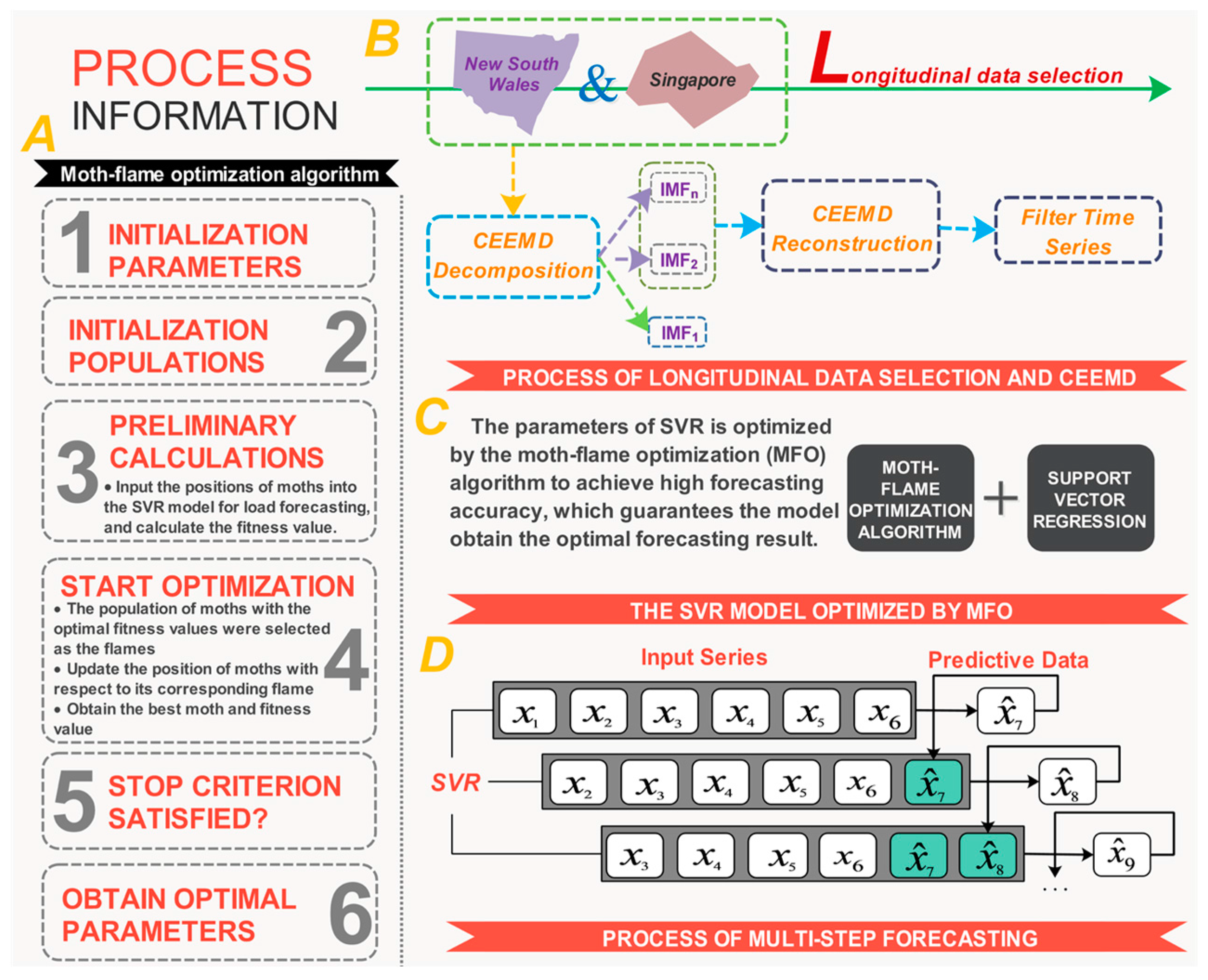
A novel hybrid model is successfully developed for multi-step short-term load forecasting; it comprises data selection, signal processing, SVR, the advanced optimization algorithm and the multi-step forecasting strategy. Its effectiveness is validated in New South Wales and Singapore.

(2)

A new intelligent optimization algorithm is initially utilized to obtain the optimal parameters of the SVR model, while the signal processing approach effectively identifies and extracts the main feature of power load series, and it is proven that these methods can improve the forecasting performance.

(3)

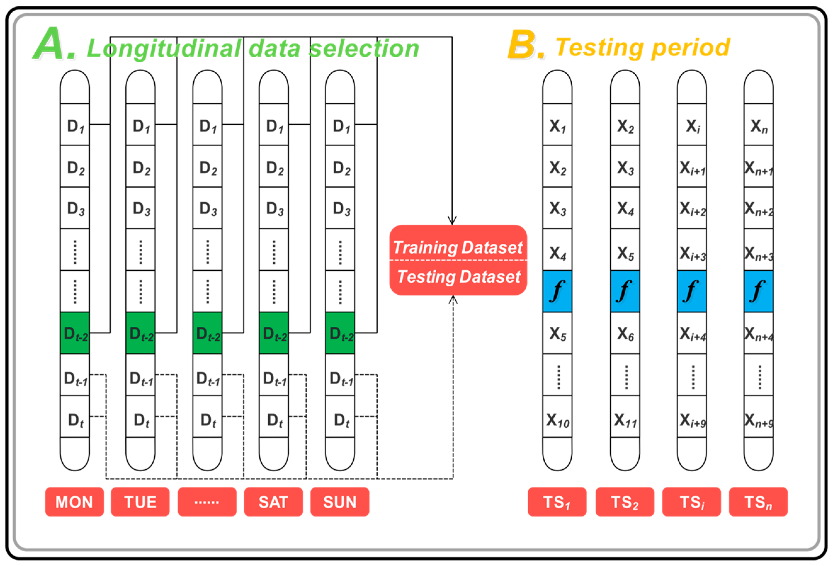
The data structure of the forecasting model is effectively constructed by the data selection, which ensures that the datasets have the same properties to achieve abundant forecasting performance.

(4)

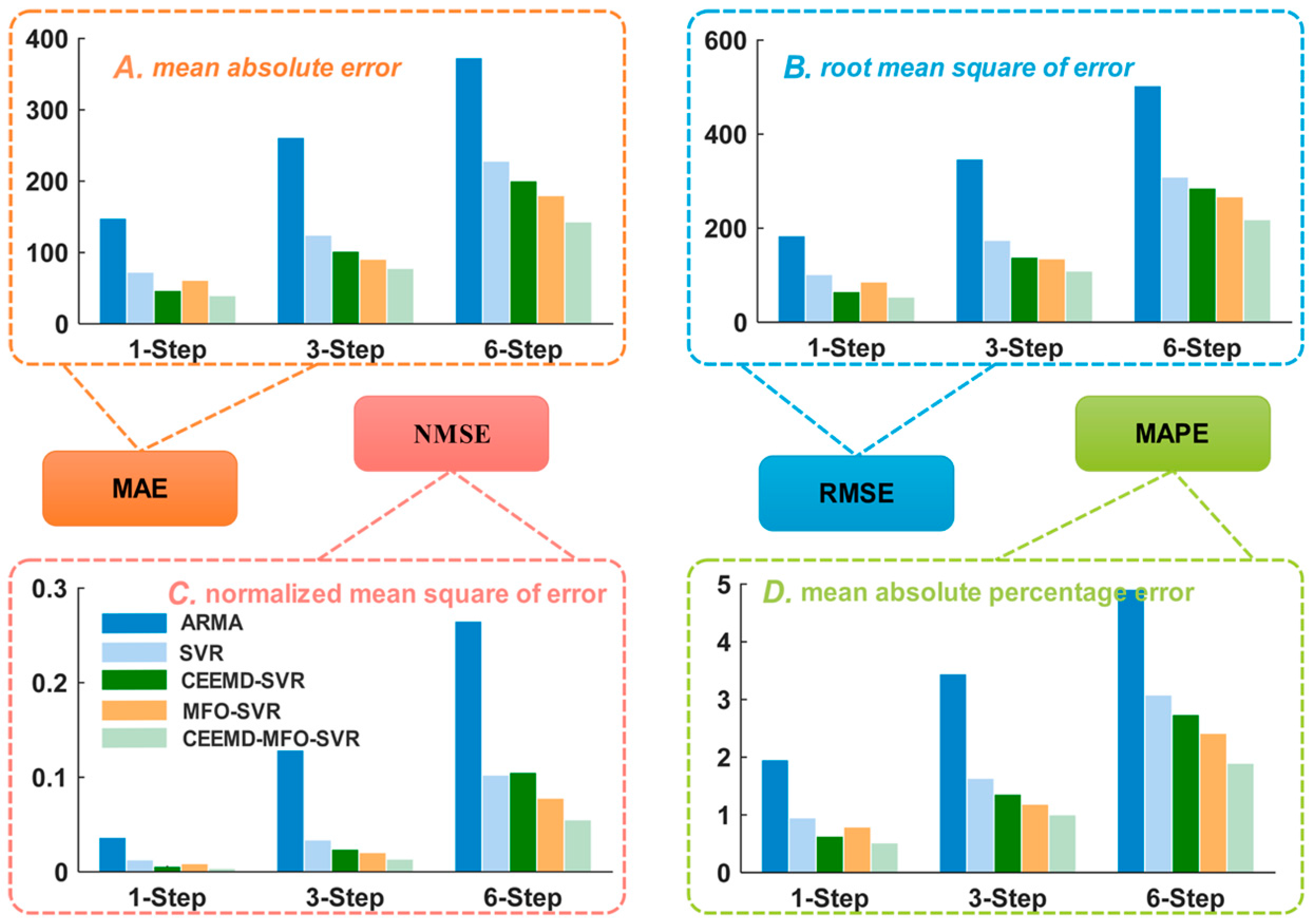
A more comprehensive evaluation of the proposed model is conducted in this paper. Two testing methods, i.e., the Diebold–Mariano (DM) test and forecasting effectiveness, are employed to evaluate the proposed hybrid model, in addition to four common metric rules, i.e., the mean absolute error (MAE), root mean square of error (RMSE), normalized mean square of error (NMSE) and mean absolute percentage error (MAPE).

In the present work, this innovative integrated model is evaluated using the half-hourly power load series of two sites, including New South Wales and Singapore, to develop a robust model to forecast the future changes in power load series. The remainder of this paper is organized as follows: a general description of the required individual tools is presented in Section 2. Section 3 describes the developed hybrid forecasting model. We present and discuss the experimental results in Section 4. Section 5 presents an insightful discussion of the experiments. Finally, Section 6 concludes the paper.

2. Methodology

In this section, a general description of the required individual tools of the novel method is presented in detail.

2.1. The Decomposition Approach for Signal Processing

The complete ensemble empirical mode decomposition (CEEMD) with adaptive noise, as a suitable signal processing approach for signal processing, is performed to decompose the original series. Compared with the traditional signal processing methods, the empirical mode decomposition (EMD) family is empirical, intuitive, direct and self-adaptive, being developed for signals featured by nonlinearity and non-stationary. In fact, most traditional signal processing algorithms perform well only under the condition that the signal satisfy certain characteristics. For example, the Fourier decomposition method is mainly employed to handle the data featuring smooth and cyclic data, while the wavelet decomposition algorithm requires non-stationary but linear data. The CEEMD technique was proposed by Torres et al. [43] to improve the decomposition methods of the EMD family. EMD was proposed by Huang et al. [44] and is used to decompose raw series into several intrinsic mode functions (IMFs) via a sifting process, which means a single mode can contain oscillations with large differences or similar oscillations can decompose between different modes [45]. To solve the disadvantage of mode mixing, ensemble empirical mode decomposition (EEMD) was developed by Wu and Huang [46]. Even if EEMD yields a substantial improvement and can improve stability significantly, it also causes a new problem: it is difficult to entirely neutralize the added noise. Therefore, Torres et al. [43] developed the CEEMD with adaptive noise to handle the defects exiting in EMD and EEMD, achieving a negligible reconstruction error and a great improvement of EEMD. With the nonlinear dynamical pattern of the power load data considered, in this work, the advanced CEEMD algorithm is adopted as the signal processing method due to its superiority to other methods. A more detailed description of this signal processing approach can be found in the literature [43].

2.2. Support Vector Regression (SVR)

The SVM, proposed by Vapnik and his co-workers, is based on structural risk minimization (SRM), which is derived from a statistical learning theory (SLT) called the Vapnik–Chervonenkis (VC) dimension theory [47]. SVM has been widely employed in various fields, such as classification, regression and non-linear function approximation. Support vector regression (SVR) is an application of SVM; the idea of SVR is to map the data into a high dimensional feature space via nonlinear mapping and to perform a linear regression in the space [48]. Moreover, it is one of the top ten models in data mining and is recommended as one of the most precise and robust algorithms among the reputable data mining algorithms [49]. It performs excellently and can be widely used in the forecasting field due to its capability to solve non-linear problems. The regression formula is defined as:

$$f\left(x\right)={\displaystyle \sum _{i=1}^D{w}_i{\mathsf{\varphi }}_i(x)+b}$$

(1)

where ${\{{\mathsf{\varphi }}_i(x)\}}_{i=1}^D$ denotes the features, b is the bias term and ${\{w_i\}}_{i=1}^D$ denotes estimated weight vectors, which can be calculated by optimizing the quadratic programming problem:

$$\begin{array}{l}\underset{w,b,\mathsf{\zeta }}{\min }\frac{1}{2}{\Vert w\Vert }^2+\mathit{C}{\displaystyle \sum _{i=1}^n\left({\mathsf{\zeta }}_i+{\mathsf{\zeta }}_i^{\ast }\right)}\\ s.t.\left|y_i-<w\cdot \mathsf{\Phi }\left(x\right)>-b\right|\le \mathsf{\epsilon }+{\mathsf{\zeta }}_i,\\ i=1,2,...,n,\mathsf{\zeta }\ge 0,{\mathsf{\zeta }}_i^{\ast }\ge 0\end{array}$$

(2)

We can convert nonlinear regression cases into linear regression cases using a kernel function k (x_i, x). The nonlinear mapping can be obtained by:

$$f\left(x,\mathsf{\alpha },{\mathsf{\alpha }}^{\ast }\right)={\displaystyle \sum _{i=1}^N\left({\mathsf{\alpha }}_i-{\mathsf{\alpha }}_i^{\ast }\right)}k\left(x_i,x\right)+b$$

(3)

Several typical kernel functions have been adopted in practical application; in this paper, the RBF kernel function is selected, which can be expressed by:

$$k\left(x_i,x\right)=\exp \left\{-\Vert x-x_i\Vert /2{\mathsf{\sigma }}^2\right\}$$

(4)

2.3. Brief Overview of Moth-Flame Optimization Algorithm

The novel natured-inspired meta-heuristic algorithm of the moth-flame optimization algorithm, which was developed by Mirjalili [50], was illuminated by the navigation approach of moths in nature, named transverse orientation. Figure 1A [50] can help us to better comprehend the mechanism of transverse orientation. As shown, the moth flies while keeping a fixed angle with respect to the moon so that it can easily achieve effective travel in a straight line, especially for a long distance from the light. In contrast, the moth will eventually converge to the light due to maintaining a similar angle when the light source is very close, as indicated in Figure 1B [50]. A general description is presented in detail [50,51], and the main steps are described as follows:

● Step 1: Set parameters

The main parameters of the moth-flame optimization algorithm include the number of moths and flames, the maximum iteration number, the number of variables and the lower/upper bound of each variable.

● Step 2: Initialize position

The moths’ and flames’ positions are obtained by:

$$\mathit{M}=\left[\begin{array}{cccc}{m}_{1,1}& m_{1,2}& \cdot \cdot \cdot & m_{1,d}\\ m_{2,1}& m_{2,2}& \cdot \cdot \cdot & m_{2,d}\\ ⋮& ⋮& ⋮& ⋮\\ m_{n,1}& m_{n,2}& \cdot \cdot \cdot & m_{n,d}\end{array}\right]$$

(5)

$$\mathit{F}=\left[\begin{array}{cccc}{F}_{1,1}& F_{1,2}& \cdot \cdot \cdot & F_{1,d}\\ F_{2,1}& F_{2,2}& \cdot \cdot \cdot & F_{2,d}\\ ⋮& ⋮& ⋮& ⋮\\ F_{n,1}& F_{n,2}& \cdot \cdot \cdot & F_{n,d}\end{array}\right]$$

(6)

where M denotes the moths’ positions, and F denotes the flames’ positions; moreover, the number of moths is n, while the number of variables is d. The initialized positions of F and M can be defined as:

$$m_{\ast ,j}\mathrm{or}{F}_{\ast ,j}=\left(u{b}_j-l{b}_j\right)\times rand\left(\right)+l{b}_j$$

(7)

where $m_{\ast ,j}$ and $F_{\ast ,j}$ are the corresponding values of M and F and the lower/upper bounds of variables are denoted as lb and ub, respectively; moreover, rand is a random number between 0 and 1.

● Step 3: Select fitness values

The fitness values of each flame can be calculated by inputting the corresponding position, which can be used to evaluate each flame. Then, the corresponding fitness values can be calculated by solving Equation (8) and are denoted as OF, which always includes n recent best solutions obtained up to now:

$$\mathit{O}\mathit{F}=\left[\begin{array}{c}O{F}_1\\ O{F}_2\\ ⋮\\ O{F}_n\end{array}\right]$$

(8)

The moth would never miss the best solution in each iteration due to selecting and saving the fitness values. The final optimal solutions obtained so far are regarded as the flames, and increase the probability of finding better solutions.

● Step 4: Iteration and optimization

The logarithmic spiral is defined to mimic the moth’s spiral flying pattern with respect to a flame, which is used to illustrate how the moths renew their positions around a flame, and can be illustrated by:

$$M_i=S\left(M_i,F_j\right)=D_i\cdot e^{bt}\cdot \cos \left(2\mathsf{\pi }t\right)+F_j$$

(9)

$$D_i=\left|F_j-M_i\right|$$

(10)

where M_i and F_j are the i-th moth and j-th flame, respectively; D_i is the distance between the moth and flame; S is the spiral function. Moreover, a constant is denoted as b, which is used to define the shape of the logarithmic spiral, and t is a random number between −1 and 1, which illustrates how close the next position should be to the flame. Specifically, t = 1 implies the farthest position from the flame, while t = −1 means the closest. However, the position updating method defined by Equation (9) will lead to convergence in local optima due to it only requiring the moths to move around a flame. To avoid dropping into a local optimum, each moth must renew its position according to only one of the flames in Equation (9). The flames will be sorted by their fitness in the iteration and after updating. Then, the moths update their positions with respect to the corresponding flames, but the updating with respect to n different positions will weaken the ability of exploiting the best solution. Therefore, an adaptive mechanism for the number of flames is employed to solve this problem. The number of flames is decreased adaptively during iterations, which is defined as:

$$flameno=\mathrm{round}\left(N-l\ast \left(N-1\right)/T\right)$$

(11)

where N is the maximum number of flames, l is the current iteration number, and T is the maximum iteration number.

● Step 5: Select optimal solutions

The flame will update its position if no one is any better than the best flame of the previous iteration; the best flame is then re-determined. Finally, the moth-flame optimization algorithm is stopped when it satisfies the termination criterion and then returns the best solution after global searching, which is considered as the optimal approximation of the optimum. The pseudo code is described as follows:

Algorithm 1 Moth-Flame Optimization Algorithm.
	Input:   $x_s^{\left(0\right)}=\left(x^{\left(0\right)}\left(1\right),x^{\left(0\right)}\left(2\right),\dots ,x^{\left(0\right)}\left(q\right)\right)$—a sequence of training data   $x_p^{\left(0\right)}=\left(x^{\left(0\right)}\left(q+1\right),x^{\left(0\right)}\left(q+2\right),\dots ,x^{\left(0\right)}\left(q+d\right)\right)$—a sequence of test data Output: $g_{best}$—the value can satisfy the best fitness after global searching
	Parameters:   n—the number of moths and flames   d—the number of variables   Max_iter—the maximum iteration number   fi—the fitness function of moth i   iter—the current iteration number   lb/ub—the lower/upper bound of variables
1	/*Set the parameters of MFO.*/
2	/*Initialize the position of moth Mi (i = 1, 2, ..., n) randomly.*/
3	FOR EACH i: 1 ≤ i ≤ n DO
27	END WHILE
28	RETURN gbest

3. The Innovative Hybrid Model for Short-Term Load Forecasting

The developed hybrid model will be expounded upon in this section; the flowchart is depicted in Figure 2. In the previous section, the methodology of the components of the model was described in detail. For the forecasting problem, the individual model pays no attention to the significance of data selection, signal processing and optimizing the model parameter; thus, the single algorithms cannot always satisfy the time series forecasting.

With these above-mentioned ignored factors considered, to enhance forecasting accuracy and stability, in this section, a novel and robust hybrid forecasting model is proposed; it combines data selection, signal processing, support vector regression (SVR) and the latest natured-inspired meta-heuristic algorithm, i.e., the moth-flame optimization algorithm. The hybrid forecasting model comprises three steps: first, the data selection method is employed to classify the original time series into some subsets, which indicates that the forecasting performance can be improved due to the dataset featuring the same properties; second, the filter time series are reconstructed by using the signal processing technique, which guarantees that the main feature (i.e., trend and seasonality) of electric power load series can be effectively identified and extracted (the procedure of the signal processing is illustrated in Figure 2B); finally, the SVR algorithm, which is optimized by the advanced optimization algorithm, is used to deal with the power load featuring irregularity and volatility. Note that, at this point, the established model can be used to realize one-step forecasting of a time series based on historical data; however, multi-step forecasting is also an increasingly critical issue in power system operation. Therefore, the integrated model, which includes the multi-step forecasting strategy, is employed to perform the multi-step forecasting, which is employed to evaluate the effectiveness of the proposed model further. In the multi-step forecasting process, the previous forecasting results will also be used to forecast the future-step results. The procedure of multi-step forecasting is illustrated in Figure 2D, which can help us to understand the realization process of multi-step forecasting well.

4. Materials and Methods

In general, except the forecasting accuracy, the stability and universality of the model to handle the short-term load forecasting issue for different datasets should also be assessed. Therefore, two different power load series of New South Wales of Australia and Singapore, which are half-hourly power load data of March and October, respectively, from 2011 to 2014, as shown is

Table 1. Statistical values of data used in this paper.

Week	Region	Mean Value (MW)	Std. Dev. (MW)	Maximum Value (MW)	Minimum Value (MW)	Median Value (MW)
MON.	New South Wales	8270.0208	1220.6354	10,621.8300	5692.5600	8571.6300
	Singapore	5407.2164	742.9222	6553.9290	3850.9450	5611.6020
TUE.	New South Wales	8469.4371	1217.0708	11,313.9900	5797.8500	8716.4100
	Singapore	5469.3661	703.0311	6594.3200	4067.8360	5602.9195
WED.	New South Wales	8461.4985	1181.7534	10,724.8600	5890.3100	8775.5750
	Singapore	5458.0263	725.8797	6615.5320	3951.9800	5558.4580
THU.	New South Wales	8472.2550	1169.9212	10,620.7600	5993.0700	8858.1650
	Singapore	5503.4093	720.7056	6605.4680	3893.7420	5683.4410
FRI.	New South Wales	8236.6968	1144.1726	10,584.6400	5728.4000	8486.0100
	Singapore	5462.0146	713.9701	6559.1230	3959.9520	5575.0105
SAT.	New South Wales	7502.7387	829.6106	9528.0100	5449.5900	7658.9200
	Singapore	5057.6897	463.4318	5972.7020	3961.5620	5105.3080
SUN.	New South Wales	7323.2883	919.6963	9960.3000	5455.5700	7444.1350
	Singapore	4816.5295	415.4188	5612.7050	3763.7360	4832.8800

, are considered as illustrative examples in this paper.

The simple map of the study area is shown in Figure 2B. Then, to determine the best experimental parameters, the trial and error method is adopted to address this problem [52]; the experimental parameters are shown in

Table 2. Experimental parameter values.

Model	Experimental Parameter	Default Value
CEEMD	Noise standard deviation	0.2
	The number of realizations	200
	The removed intrinsic mode functions	IMF1
	Maximum number of sifting iterations	5000
MFO	The number of search agents	30
	Maximum number of iterations	300
	The lower bounds of variables	0.01
	The upper bounds of variables	100
	The number of variables	2
	The convergence constant r	−1 to −2
SVR	The number of the input layer	4
	The number of the output layer	1
	The kernel function’s name	RBF
	The cost c of original the SVR	1
	The gamma g of original the SVR	0.25

. All experiments were carried out in MATLAB R2014a on Windows 7 with a 3.30 GHz Intel Core i5 4590, 64 bit computer equipped with 8 GB RAM.

4.1. Data Selection

Data selection plays a key role in the forecasting issue. There are many factors that randomly influence the power data, which leads the data to present different characteristics. Hence, we should divide the raw data series into different datasets according to a certain suitable method and separately build the forecasting model for the power data. To enhance forecasting performance and guarantee the adaptability of the novel hybrid model applied in STLF, longitudinal data selection is employed in this paper. In detail, we first classify the original data according to the month; then, the datasets are divided into seven subsets according to a particular day of one week, which ensures that each subset has the same inner characteristics and thus improves the forecasting performance. The longitudinal data selection process for power load series is shown in Figure 3A. For example, there are 18 Sundays of March in total (48 data points per day) from 2011 to 2014, which are treated as one subset; the other subset is similarly constructed. For each subset, the last 2 days are the testing sample, while the remainder is the training sample.

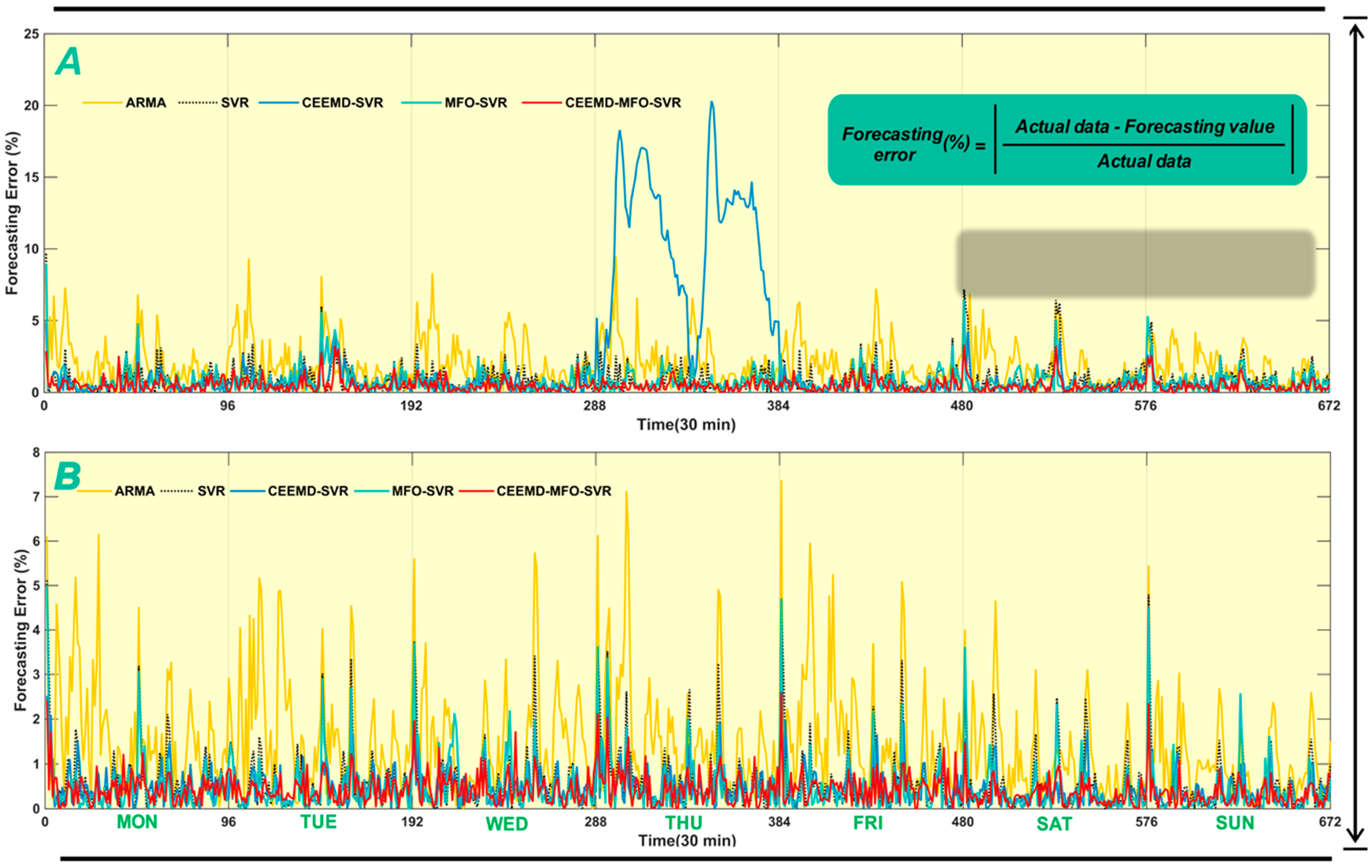
4.2. The Performance Metric

To evaluate the forecasting performance and comprehensively learn the model traits better, four performance metric rules, which are presented in

Table 3. Four performance metric rules.

Metric	Definition	Equation
MAE	The mean absolute error of N forecasting results	$\mathbf{M}\mathbf{A}\mathbf{E}=\frac{1}{N}{\displaystyle \sum _{i=1}^N\left|F_i-A_i\right|}$
RMSE	The square root of average of the error squares	$\mathbf{R}\mathbf{M}\mathbf{S}\mathbf{E}=\sqrt{\frac{1}{N}\times {\displaystyle \sum _{i=1}^N{\left(F_i-A_i\right)}^2}}$
NMSE	The normalized average of the squares of the errors	$\mathbf{N}\mathbf{M}\mathbf{S}\mathbf{E}=\frac{1}{N}{\displaystyle \sum _{i=1}^N\frac{{\left(F_i-A_i\right)}^2}{F_i{A}_i}}$
MAPE	The average of N absolute percentage error	$\mathbf{M}\mathbf{A}\mathbf{P}\mathbf{E}=\frac{1}{N}{\displaystyle \sum _{i=1}^N\left|\frac{A_i-F_i}{A_i}\right|}\times 100\%$

, are employed in this paper: N is the length of data to evaluate; F is the forecasted value; A represents the observed value. Smaller index values represent better forecasting performance.

4.3. Testing Method

The model performance evaluation metrics presented in Section 4.2 have great significance in comparing the different forecasting models. However, to verify the outstanding performance, testing needs to be done from the statistical perspective. Therefore, the Diebold–Mariano (DM) test and forecasting effectiveness are conducted in this paper as two testing methods for further performance comparison studies.

4.3.1. DM Test

The Diebold-Mariano (DM) test [53] was used to compare and evaluate the significance of the outperformance of the proposed model with other comparable models. Assume that two forecasting models are compared and evaluated: model A and model B.

Actual values:

$$\left\{y_n;n=1,\dots ,t+k\right\}$$

(12)

Forecast values:

$$\left\{{\widehat{y}}_n^{(A)};n=1,\dots ,t+k\right\},\left\{{\widehat{y}}_n^{(B)};n=1,\dots ,t+k\right\}$$

(13)

Forecast errors:

$${\mathsf{\epsilon }}_{t+h}^{(A)}=y_{t+h}-{\widehat{y}}_{t+h}^{(A)},h=1,2,\dots ,k.$$

(14)

$${\mathsf{\epsilon }}_{t+h}^{(B)}=y_{t+h}-{\widehat{y}}_{t+h}^{(B)},h=1,2,\dots ,k$$

(15)

The loss function $L\left({\mathsf{\epsilon }}_{t+h}\right)$ is employed to measure the forecasting accuracy of different models. Two popular versions of the loss function are presented below:

Absolute deviation loss:

$$L\left({\mathsf{\epsilon }}_{t+h}\right)=\left|{\mathsf{\epsilon }}_{t+h}\right|$$

(16)

Square error loss:

$$L\left({\mathsf{\epsilon }}_{t+h}\right)={\left({\mathsf{\epsilon }}_{t+h}\right)}^2$$

(17)

The DM test statistic values can be calculated by:

$$DM=\frac{{\displaystyle \sum _{h=1}^k\left(L\left({\mathsf{\epsilon }}_{t+h}^{(A)}\right)-L\left({\mathsf{\epsilon }}_{t+h}^{(B)}\right)\right)/k}}{\sqrt{S^2/k}}{s}^2$$

(18)

where S² is an estimation of the variance of $d_h=L\left({\mathsf{\epsilon }}_{t+h}^{(A)}\right)-L\left({\mathsf{\epsilon }}_{t+h}^{(B)}\right)$. The hypothesis test is:

$$H_0:E\left(d_h\right)=0,\forall n$$

(19)

$$H_1:E\left(d_h\right)\ne 0,\exists n$$

(20)

The test statistic DM is convergent in distribution in the standard normal distribution N (0, 1). The null hypothesis will be rejected if:

$$\left|DM\right|>z_{\mathsf{\alpha }/2}$$

(21)

where z_α/2 denotes the critical z-value of the standard normal distribution and α is the significance level.

4.3.2. Forecasting Effectiveness

The forecasting effectiveness was employed to verify the forecasting accuracy of the developed hybrid model and other compared models. It is often the case that 1st-order and 2nd-order forecasting effectiveness are available for forecasting evaluation in empirical applications. A general description of forecasting effectiveness is presented in detail [54]:

Actual values:

$$\left\{y_n;n=1,\dots ,N\right\}$$

(22)

Forecast values:

$$\left\{{\widehat{y}}_n;n=1,\dots ,N\right\}$$

(23)

Forecast errors:

$${\mathsf{\epsilon }}_n=y_n-{\widehat{y}}_n$$

(24)

Forecast accuracy:

$$A_n=\{\begin{array}{cc}1-\left|\frac{{\mathsf{\epsilon }}_n}{y_n}\right|,\hfill & \hfill 0\le \left|\frac{{\mathsf{\epsilon }}_n}{y_n}\right|\le 1\\ 0,\hfill & \hfill \left|\frac{{\mathsf{\epsilon }}_n}{y_n}\right|>1\end{array}$$

(25)

The k-th-order forecasting effectiveness unit is calculated by:

$$m^k={\displaystyle \sum _{n=1}^N{Q}_{n}A{}_n^k}$$

(26)

where k is a positive integer and $Q_n$, which indicates the discrete probability distribution at time n, is a positive number; ${\displaystyle \sum _{n=1}^N{Q}_n=1}$. If the priori information of the discrete probability distribution cannot be known, $Q_n$ is defined as a constant equals to 1/N. The kth-order forecasting effectiveness is defined as:

$$H\left(m^1,m^2,\cdots ,m^k\right)$$

(27)

where H is a continuous function of a certain k unit. Especially if $H\left(x\right)=x$ is a continuous function with one variable, the 1st-order forecasting effectiveness is the expectation forecasting accuracy sequence, defined as $H\left(m^1\right)=m^1$; meanwhile, $H\left(x,y\right)=x\left(1-\sqrt{y-x^2}\right)$ is a continuous function with two variables. The 2nd-order forecasting effectiveness is the difference between the expectation and standard deviation, presented as $H\left(m^1,m^2\right)=m^1\left(1-\sqrt{m^2-{\left(m^1\right)}^2}\right)$.

4.4. Experiment I: The Case of New South Wales

This half-hourly power load series was collected in March from 2011 to 2014 in New South Wales. As mentioned above, longitudinal data selection is employed to split the original dataset into seven subsets to guarantee that each subset has the same characteristics, which can yield forecasting performance improvements. Each subset is divided into two parts, as shown in Figure 3A; the last 2 days are the testing sample and the remainder is the training sample. For example, there are 17 Mondays of March in total from 2011 to 2014; the former 15 days are the training set while the last 2 days are the testing set; the other subset is similarly constructed. To verify the forecasting performance, four performance metrics (i.e., MAE, NMSE, RMSE, MAPE) for each subset are calculated and presented in

Table 4. The results of the proposed model and the results of the other models (Experiment I).

Week	Metric	ARMA			SVR			CEEMD-SVR			MFO-SVR			CEEMD-MFO-SVR
		1-Step	3-Step	6-Step	1-Step	3-Step	6-Step	1-Step	3-Step	6-Step	1-Step	3-Step	6-Step	1-Step	3-Step	6-Step
MON.	MAE	149.3168	264.3664	414.2613	72.0154	136.3824	268.4663	45.8432	101.7635	211.1696	64.7532	109.1297	252.7814	42.0844	78.7812	150.1316
	RMSE	189.2493	361.0766	555.7324	109.0032	206.5667	380.2364	65.6234	136.8509	275.2133	97.5332	180.4214	401.6520	56.8869	108.8300	227.2187
	NMSE	0.0301	0.1097	0.2599	0.0100	0.0359	0.1217	0.0036	0.0158	0.0637	0.0080	0.0274	0.1358	0.0027	0.0100	0.0434
	MAPE	1.9765	3.4818	5.5275	0.9450	1.8508	3.7417	0.6085	1.3670	2.8341	0.8479	1.4915	3.6348	0.5395	1.0160	1.9835
TUE.	MAE	155.7903	273.7074	416.3040	82.4250	168.1516	345.1775	62.6412	154.0930	310.9179	74.8796	128.7659	211.1475	45.2562	97.7580	153.5884
	RMSE	197.0058	366.0849	578.0620	109.7363	234.6780	439.8573	82.8290	213.9505	424.9461	101.7121	184.8466	293.0550	62.0565	136.4468	222.9660
	NMSE	0.0364	0.1257	0.3135	0.0113	0.0517	0.1815	0.0064	0.0429	0.1694	0.0097	0.0321	0.0806	0.0036	0.0175	0.0466
	MAPE	2.0502	3.6205	5.5876	1.0651	2.2069	4.6264	0.8354	2.0455	4.1823	0.9940	1.7304	2.8821	0.5975	1.2716	2.1002
WED.	MAE	164.0952	299.0298	464.1855	68.9116	123.8473	249.4280	44.4607	97.5785	193.3782	55.3373	82.1219	157.8759	36.5947	76.2369	129.8791
	RMSE	201.2296	382.5640	592.0291	88.4652	162.6603	319.5566	57.1206	131.0734	256.0120	72.4172	114.9260	216.5579	49.0040	107.0317	194.0142
	NMSE	0.0342	0.1235	0.2957	0.0066	0.0223	0.0862	0.0028	0.0145	0.0553	0.0044	0.0111	0.0396	0.0020	0.0097	0.0318
	MAPE	2.0936	3.7744	5.8298	0.8628	1.5552	3.2686	0.5619	1.2362	2.5270	0.6848	1.0060	1.9699	0.4598	0.9527	1.6581
THU.	MAE	167.7732	288.0813	406.8082	69.7697	121.9849	227.0328	46.5032	90.8335	175.0757	61.7127	75.8345	170.5123	38.2440	79.3382	150.2177
	RMSE	207.8787	385.7540	539.3338	90.6257	169.2368	312.8293	68.0893	121.3090	274.4343	79.6795	108.7897	264.7262	47.4928	114.1213	247.6543
	NMSE	0.0373	0.1283	0.2508	0.0071	0.0247	0.0844	0.0089	0.0282	0.1442	0.0055	0.0102	0.0604	0.0019	0.0112	0.0529
	MAPE	2.1296	3.6411	5.1752	0.8621	1.5499	3.0098	0.6555	1.2672	2.5200	0.7390	0.9029	2.0826	0.4680	0.9604	1.8132
FRI.	MAE	151.8488	265.2930	370.4275	65.8305	99.9089	174.9614	40.6910	90.9959	163.8359	56.5212	84.0547	176.1757	39.7423	65.0562	132.6612
	RMSE	181.5484	362.8613	525.1881	90.2945	148.2388	250.2056	53.0908	122.9946	221.1164	78.4528	131.1631	255.4916	52.8244	86.6114	173.2087
	NMSE	0.0338	0.1352	0.2833	0.0084	0.0226	0.0643	0.0029	0.0155	0.0502	0.0063	0.0177	0.0670	0.0029	0.0077	0.0308
	MAPE	1.9485	3.4052	4.7655	0.8377	1.2605	2.2791	0.5203	1.1610	2.1590	0.7121	1.0669	2.2727	0.5100	0.8091	1.7047
SAT.	MAE	125.8284	219.3056	248.4333	78.5700	116.2084	147.3141	41.5799	84.2632	163.6957	51.6702	76.7323	137.7728	36.3863	71.8198	132.2958
	RMSE	160.6073	290.5429	353.8855	123.6085	159.9216	210.5417	65.4166	112.5968	271.2540	81.5617	113.0028	213.9510	52.1449	97.1539	202.4365
	NMSE	0.0494	0.1616	0.2398	0.0293	0.0490	0.0849	0.0082	0.0243	0.1409	0.0127	0.0244	0.0876	0.0052	0.0181	0.0785
	MAPE	1.7764	3.1003	3.4207	1.0970	1.5979	2.0595	0.5844	1.1630	2.3551	0.7032	1.0436	1.9500	0.5030	0.9768	1.8558
SUN.	MAE	116.2149	214.7425	285.9453	64.3232	97.9753	178.3560	40.7161	87.7273	179.1373	56.4753	72.0519	146.0067	33.2267	69.1963	146.1253
	RMSE	141.1563	272.2281	368.7920	89.1827	129.8764	241.5235	55.8503	121.1988	265.7823	80.2555	102.0070	213.8716	45.7782	102.7112	251.3388
	NMSE	0.0305	0.1135	0.2083	0.0122	0.0258	0.0893	0.0048	0.0225	0.1082	0.0099	0.0159	0.0701	0.0032	0.0162	0.0968
	MAPE	1.6447	3.0340	4.0101	0.9087	1.3551	2.5063	0.5767	1.2119	2.5345	0.7959	0.9927	2.0366	0.4703	0.9570	2.0863

for comparative performance studies. Furthermore, Figure 4A shows the one-step forecasting error of all models from Monday to Sunday in New South Wales. It is visible that the forecasting error line of the proposed model is clearly closest to the zero line with the lowest volatility among all the models. Moreover, Figure 5 illustrates the average values of MAE, RMSE and MAPE in New South Wales, which can be regarded as the overall forecasting potential. To gather more detailed comparison information, the one-step and six-step forecasting results of three randomly selected days (i.e., Monday, Wednesday, Friday) are depicted in Figure 6 and Figure 7, respectively; they reveal that the forecasting line of the proposed model is closer to the actual line than that of the benchmark model. Accordingly, we can conclude that the proposed hybrid model achieves the best values of all criteria in the comparative performance studies, which indicates that the proposed integrated model is superior to the traditional time series model ARMA, single artificial intelligence forecasting model SVR and two-component models CEEMD-SVR and MFO-SVR in all horizons for short-term load forecasting. More detailed comparative studies are conducted from two aspects: one-step forecasting and multi-step forecasting.

4.4.1. Analysis for One-Step Forecasting

The one-step forecasting results of each model are presented in Table 4 and Figure 4, Figure 5 and Figure 6. The experimental results indicate that this proposed hybrid model outperforms other benchmark models based on comparison of the MAE, NMSE, RMSE and MAPE. For more detailed analysis, take the forecasting result of Mondays as an example:

(a)

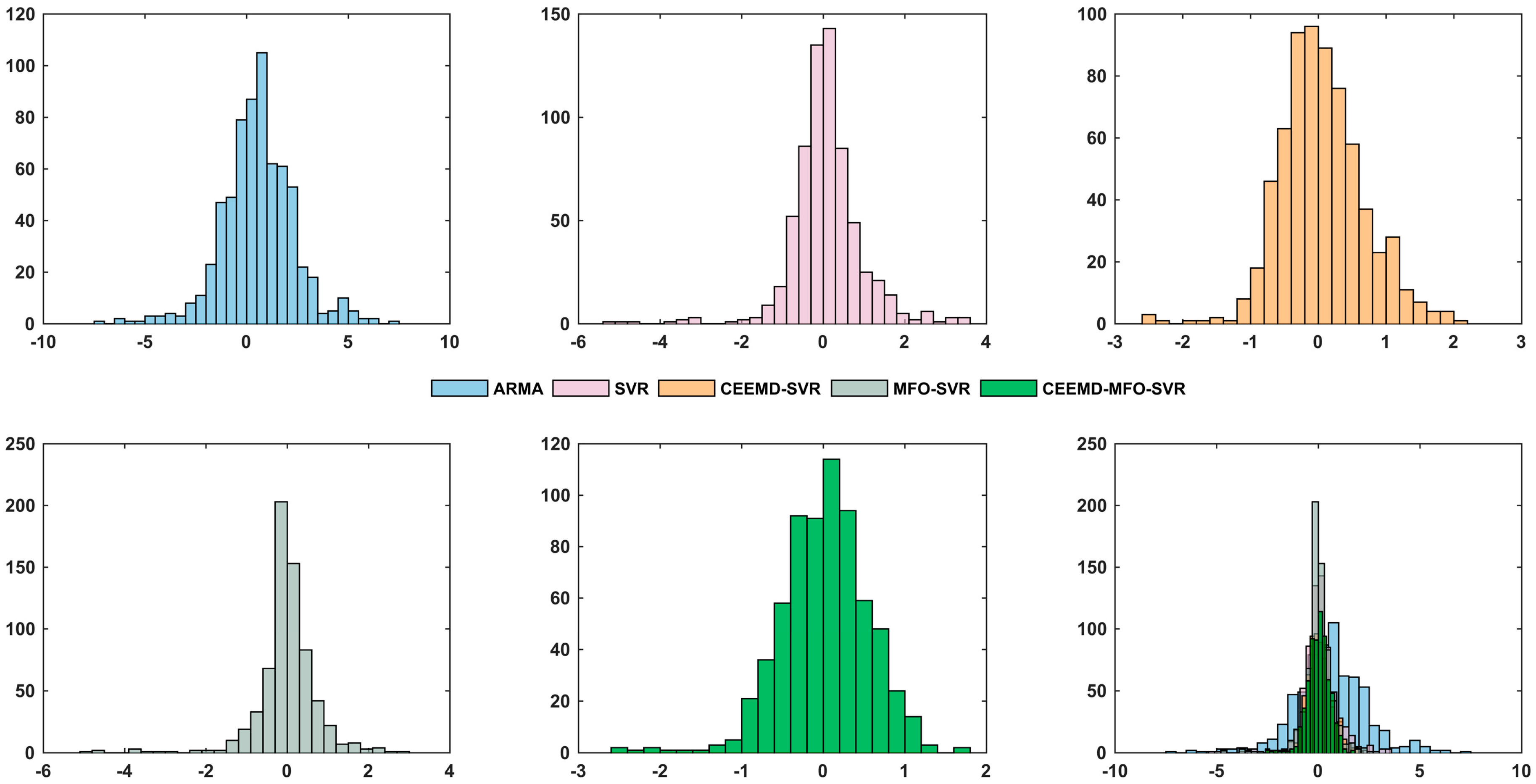
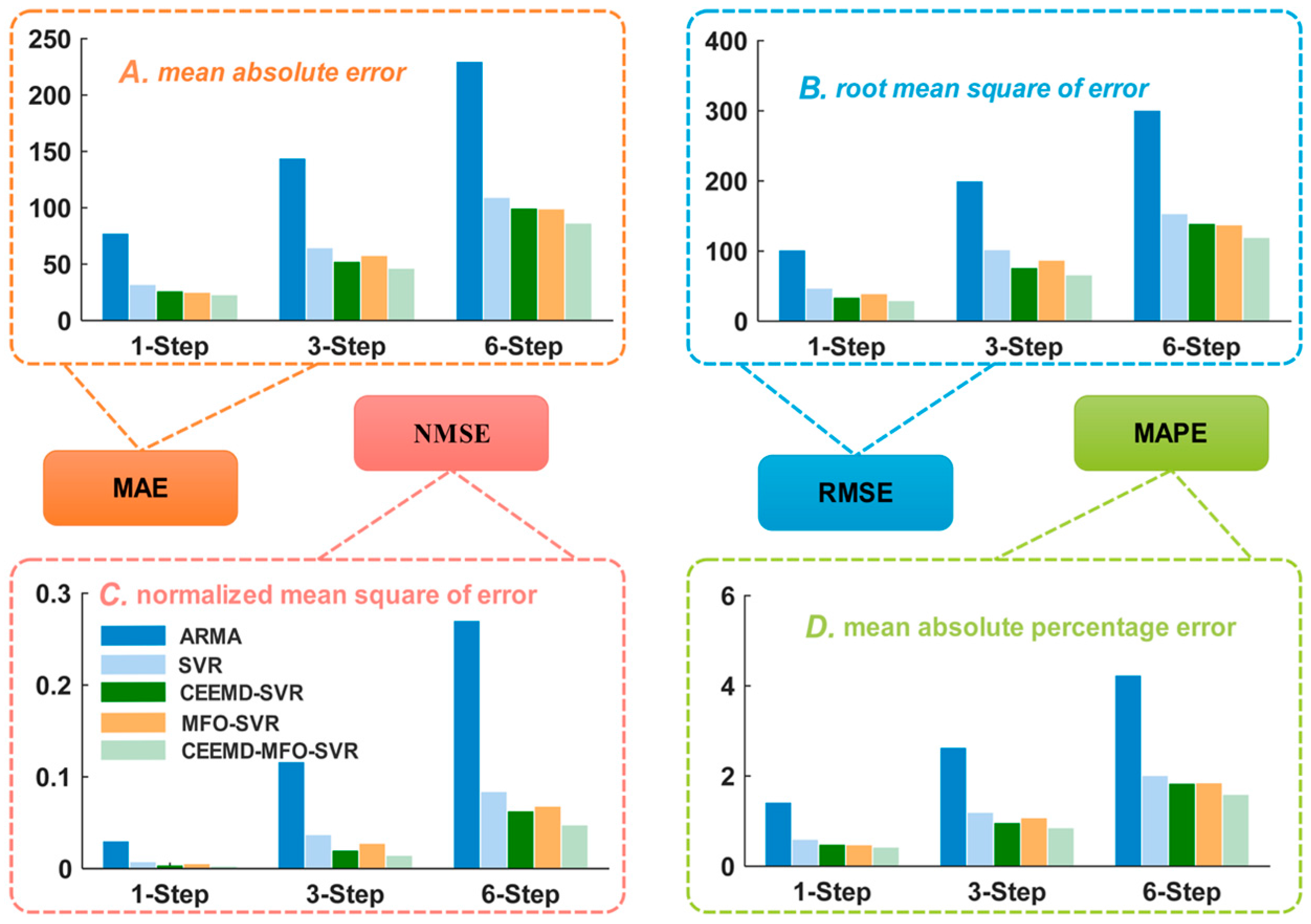
When comparing the traditional time series model ARMA with the individual artificial intelligence model SVR, regarding the MAE, NMSE, RMSE and MAPE, the SVR model is superior to the ARMA model. The results indicate that the artificial intelligent algorithms are powerful forecasting tools with strong robustness and fault tolerance to solve the STLF problem influenced by several factors, being able to achieve better performance compared with the traditional time series model.

(b)

Statistics of single SVR and our proposed model show that the integrated method leads to reductions of 29.9310 in MAE, 52.1163 in RMSE, 0.0073 in NMSE, and 0.4055% in MAPE. Moreover, the results between the individual SVR and CEEMD-SVR model reveal that the technique contributes to performance improvements of 26.1722 in MAE, 43.3798 in RMSE, 0.0064 in NMSE, and 0.3365% in MAPE. Furthermore, the results between the single SVR and MFO-SVR models demonstrate that the moth-flame optimization algorithm leads to reductions of 7.2622 in MAE, 11.4700 in RMSE, 0.0020 in NMSE, and 0.0971% in MAPE.

(c)

Statistics of different models show that the proposed model has a lower MAPE value of 0.5395% compared to the MAPEs of 1.9765%, 0.9450%, 0.6085% and 0.8479% for the ARMA, SVR, CEEMD-SVR and MFO-SVR models, respectively, which show that the integrated method leads to reductions of 1.4370%, 0.4055%, 0.0690% and 0.3084% in MAPE when compared with the ARMA, SVR, CEEMD-SVR and MFO-SVR model, respectively.

(d)

The comparison between the SVR, CEEMD-SVR, MFO-SVR and the proposed model proves that the single SVR model is inferior to the benchmark models, which proves that the signal processing and moth-flame optimization algorithm are effective in improving the forecasting accuracy. Therefore, to solve the short-term load forecasting problem, an increasing number of studies have proposed the signal processing technique and artificial intelligence optimization algorithm.

4.4.2. Analysis for Multi-Step Forecasting

Multi-step forecasting plays a vital role in the power system operation. Therefore, the hybrid model, combined with the multi-step forecasting strategy, is employed to perform the multi-step forecasting in this paper, which is employed to evaluate the effectiveness of the developed hybrid model further. The three-step and six-step forecasting results of different models are shown in Table 4 and Figure 5 and Figure 7. The results reveal that the proposed model also performs better than other benchmark models. More comparison research is illustrated below.

(a)

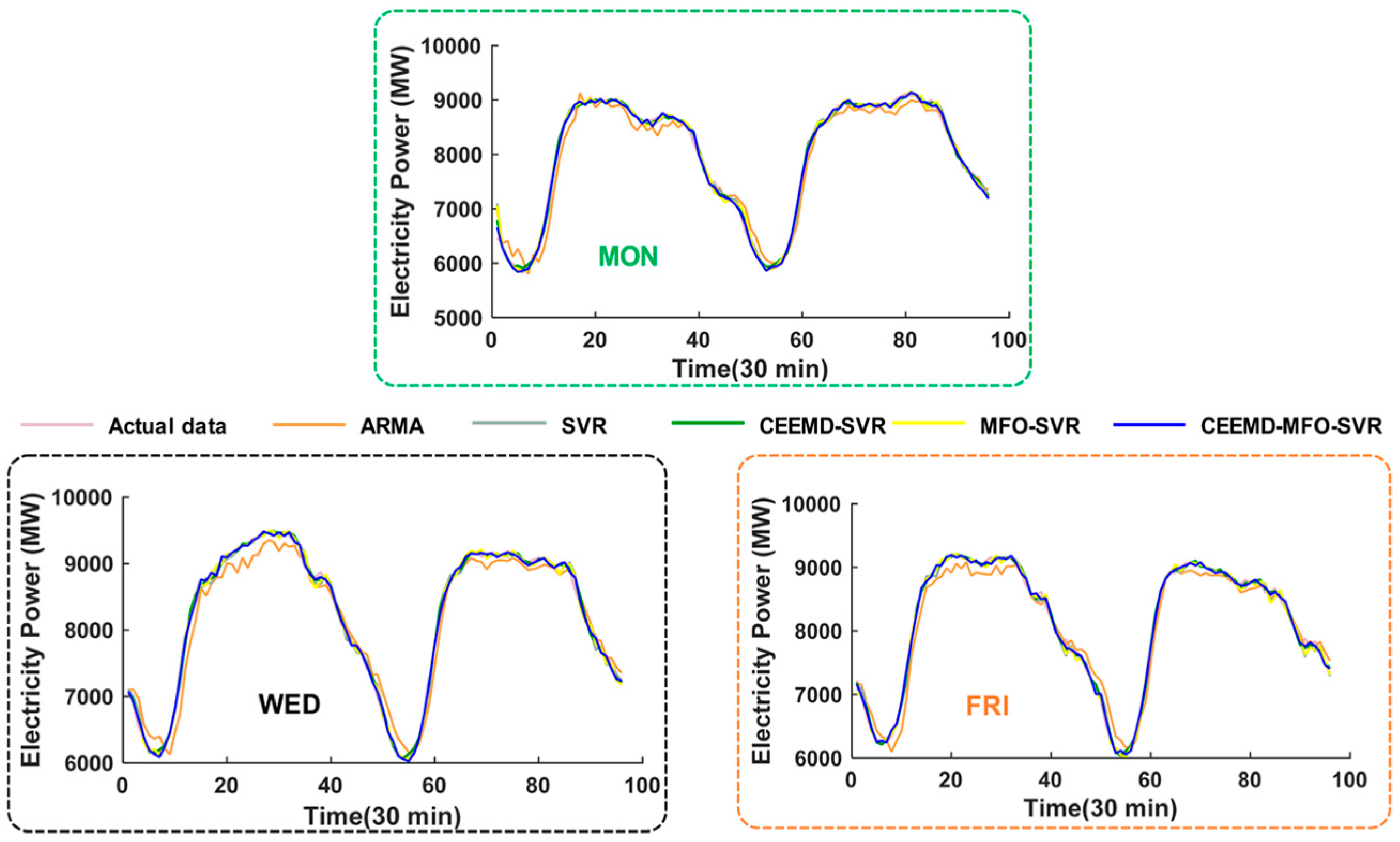
The comparison results between the ARMA model and single SVR model indicate that the SVR model can achieve better performance compared with the traditional time series model. For instance, the decreased error of MAPE for three-step forecasting is 1.6310%, 1.4136%, 2.2192%, 2.0912%, 2.1447%, 1.5024% and 1.6789%, corresponding to reductions for six-step forecasting of 1.7858%, 0.9612%, 2.5612%, 2.1654%, 2.4864%, 1.3612% and 1.5038% from Monday to Sunday, respectively.

(b)

Taking Monday as an example, the MAPE of the individual SVR model is 1.8508% in three-step forecasting and 3.7417% in six-step forecasting, while the corresponding MAPE of the proposed hybrid model is 1.0160% and 1.9835%. Moreover, compared with the CEEMD-SVR model and MFO-SVR model, the proposed model leads to reductions of 0.3510% and 0.4755% in MAPE for three-step forecasting and reductions of 0.8506% and 1.6513% for six-step forecasting, respectively, which proves that these two methods can improve the multi-step forecasting accuracy of short-term load forecasting.

(c)

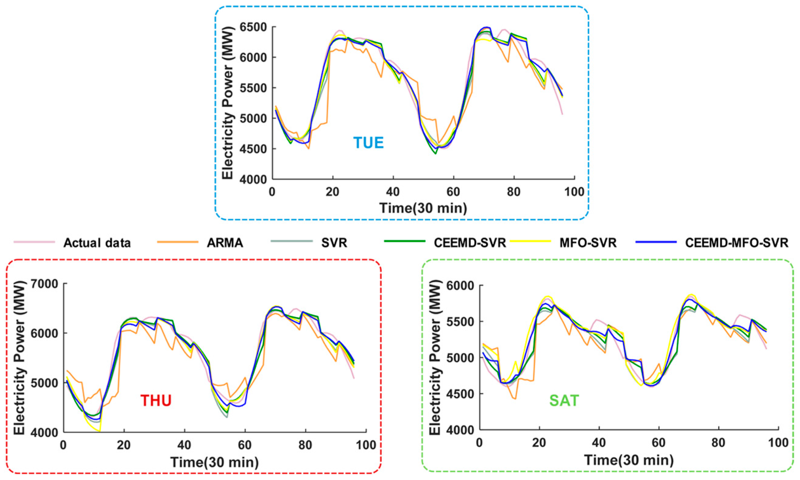
When comparing the different forecasting horizons, we can conclude that the forecasting error will increase with increasing number of rolling processes. Nevertheless, the negative influence of accumulated error can be reduced due to the SVR model’s excellent performance for one-step forecasting; thus, the proposed integrated model obtains the optimal results.

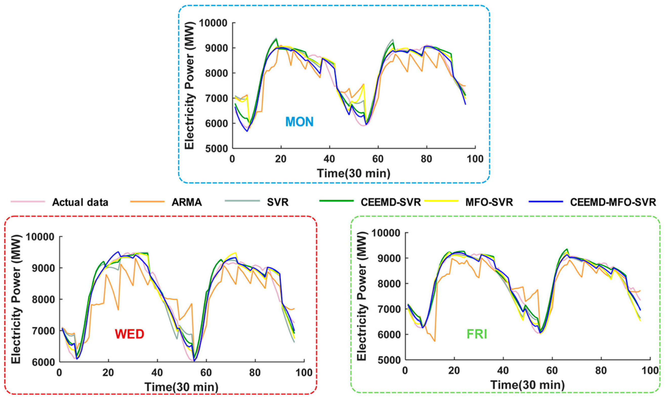
(d)

Taking Wednesday as an example, for the three-step forecasting, the proposed model has a lower MAPE value of 0.9527% compared to the MAPEs of 3.7744%, 1.5552%, 1.2362% and 1.0060% for the ARMA, SVR, CEEMD-SVR and MFO-SVR models, respectively, while also having a lower MAPE value of 1.6581% compared to the MAPEs of 5.8298%, 3.2686%, 2.5270% and 1.9699% for the ARMA, SVR, CEEMD-SVR and MFO-SVR models for six-step forecasting, respectively. The corresponding difference between three-step and six step forecasting is 0.7054%, 2.0554%, 1.7134%, 1.2908% and 0.9639%, which indicates that the proposed hybrid model is superior to other benchmark models for multi-step forecasting.

Remark 1.

Through the above case study, we compare the MAE, RMSE, NMSE and MAPE; whether for one-step forecasting or multi-step forecasting, the proposed integrated model performs better with respect to almost all. Therefore, the proposed hybrid model has better accuracy than the other models. Moreover, the signal processing algorithm, which successfully extracts the trend and volatility in the original power load series, has higher contributions than the moth-flame optimization algorithm employed to obtain the optimal parameters of SVR. Furthermore, the SVR model can effectively improve forecasting accuracy due to the dataset structures being optimal by using the longitudinal data selection method. In summary, the combination of meritorious components capitalizes on each component’s advantages, which is an effective method for STLF and can effectively forecast the power load in the future.

4.5. Experiment II: The Case of Singapore

To further verify the effectiveness of the proposed hybrid model, half-hourly load data collected in October from 2011 to 2014 in Singapore are used as another case in this section. It is well known that these two sites have a remarkably different nature and social environment; thus, we can conclude that the hybrid model has universal applicability under the condition that the hybrid model performs better at both sites. The process of the dataset structure is the same as for New South Wales. The experiment results comparing the models’ performances are presented in

Table 5. The results of the proposed model and the results of the other models (Experiment II).

Week	Metric	ARMA			SVR			CEEMD-SVR			MFO-SVR			CEEMD-MFO-SVR
		1-Step	3-Step	6-Step	1-Step	3-Step	6-Step	1-Step	3-Step	6-Step	1-Step	3-Step	6-Step	1-Step	3-Step	6-Step
MON.	MAE	90.8506	177.8643	298.7605	36.1058	70.3113	114.0703	29.8413	59.6216	113.5754	25.5246	50.6785	81.4193	25.0462	46.6848	88.0659
	RMSE	116.6122	235.4940	382.2163	51.6419	100.9278	157.6169	37.9260	80.3783	154.3141	40.8566	75.3779	117.7296	31.5145	66.2984	129.6388
	NMSE	0.0274	0.1118	0.2944	0.0054	0.0205	0.0501	0.0029	0.0130	0.0480	0.0034	0.0115	0.0279	0.0020	0.0089	0.0339
	MAPE	1.6244	3.1825	5.4467	0.6575	1.2677	2.0517	0.5328	1.0736	2.0887	0.4747	0.9354	1.4828	0.4499	0.8310	1.5995
TUE.	MAE	90.0534	156.0882	230.2655	31.5554	62.3240	105.6896	28.0266	50.5870	93.9458	23.9893	51.9725	90.2592	23.7795	43.9501	76.1427
	RMSE	116.9971	214.4720	304.2786	44.2051	99.3649	149.7291	34.8524	71.0920	126.3075	35.0084	81.0353	119.6260	28.3290	60.9403	101.6079
	NMSE	0.0309	0.1039	0.2092	0.0044	0.0223	0.0507	0.0027	0.0114	0.0360	0.0028	0.0148	0.0323	0.0018	0.0084	0.0233
	MAPE	1.6081	2.7657	4.1177	0.5647	1.1037	1.8564	0.4973	0.8970	1.6590	0.4341	0.9204	1.5912	0.4227	0.7722	1.3345
WED.	MAE	75.8072	146.4575	243.4885	31.2881	65.5748	118.0987	26.5597	53.9255	122.3793	30.0861	74.0752	130.3961	24.2925	54.2744	106.6510
	RMSE	100.4353	201.8140	317.6453	45.7135	103.8682	165.4857	32.9656	79.8731	172.3282	43.2920	111.8104	200.0023	30.8272	76.5508	153.3729
	NMSE	0.0249	0.1006	0.2492	0.0052	0.0266	0.0676	0.0027	0.0158	0.0733	0.0046	0.0309	0.0988	0.0023	0.0145	0.0581
	MAPE	1.3857	2.6743	4.4604	0.5831	1.2086	2.1834	0.4933	0.9957	2.2921	0.5726	1.3896	2.4450	0.4598	1.0141	1.9760
THU.	MAE	84.2323	162.8808	260.7049	36.7486	69.1145	124.4287	30.2405	55.6085	101.6196	30.3294	62.2568	116.7772	26.0944	51.1396	99.2455
	RMSE	112.8961	231.7337	337.2167	52.1014	107.0442	168.4231	38.3211	79.1465	143.0002	43.6659	83.9015	148.8143	34.1613	72.2945	129.8003
	NMSE	0.0257	0.1084	0.2296	0.0055	0.0231	0.0573	0.0030	0.0126	0.0413	0.0038	0.0142	0.0447	0.0024	0.0106	0.0340
	MAPE	1.5349	2.9529	4.7696	0.6787	1.2629	2.2944	0.5469	1.0128	1.8428	0.5679	1.1415	2.1601	0.4775	0.9220	1.7725
FRI.	MAE	93.7558	164.1123	242.0319	35.6067	62.9099	90.4895	29.4234	55.0429	98.3395	24.0077	57.6159	82.4145	26.2520	50.4998	82.5722
	RMSE	122.2762	237.3645	324.8348	51.5711	100.0427	130.1977	38.4653	77.4244	141.6382	39.1546	85.0135	111.3450	33.1148	67.0101	112.8754
	NMSE	0.0298	0.1123	0.2103	0.0053	0.0200	0.0338	0.0029	0.0119	0.0400	0.0031	0.0144	0.0247	0.0022	0.0090	0.0254
	MAPE	1.6684	2.9542	4.4239	0.6466	1.1238	1.6105	0.5288	0.9795	1.7646	0.4336	1.0281	1.4682	0.4682	0.8971	1.4722
SAT.	MAE	54.4423	97.7853	166.7009	24.9204	63.0766	105.8425	17.9275	46.5558	86.8615	19.8955	51.1122	103.2263	16.0642	39.9372	68.3689
	RMSE	71.2142	138.6945	215.8981	39.9705	106.8964	151.3951	25.0724	75.3149	125.1431	32.4203	83.4907	140.1891	20.7835	61.6914	98.5601
	NMSE	0.0322	0.1223	0.2964	0.0102	0.0727	0.1457	0.0040	0.0361	0.0996	0.0067	0.0443	0.1250	0.0027	0.0242	0.0618
	MAPE	1.0471	1.8696	3.1879	0.4783	1.2007	1.9987	0.3425	0.8869	1.6487	0.3877	1.0019	2.0288	0.3087	0.7771	1.3341
SUN.	MAE	50.3933	100.1250	164.2336	24.4459	55.8543	102.6142	19.4632	42.9000	78.5588	18.7082	52.5313	86.0579	15.4955	34.6784	80.5646
	RMSE	65.8844	135.3373	218.6276	40.3635	91.5260	146.4708	26.4746	66.6591	108.4774	34.7743	83.9519	119.1154	21.7158	52.4386	105.9001
	NMSE	0.0362	0.1529	0.3991	0.0136	0.0699	0.1791	0.0059	0.0371	0.0982	0.0101	0.0588	0.1185	0.0039	0.0230	0.0936
	MAPE	0.9997	1.9792	3.1899	0.4850	1.1087	2.0045	0.3860	0.8489	1.5255	0.3740	1.0447	1.6950	0.3088	0.6925	1.5907

, Figure 4B and Figure 8, Figure 9 and Figure 10. The one-step forecasting errors of different models from Monday to Sunday are presented in Figure 4B. It is obvious that the forecasting result is very approximate to the target, while the forecasting error line of the proposed model is clearly closest to the zero lines, with the lowest volatility among all the models. Figure 8 shows the average value of MAE, RMSE and MAPE in Singapore, which also represents the overall ability for power load forecasting. Furthermore, to analyze the forecasting result in detail, Figure 7 and Figure 8 depict the results of three randomly selected days (i.e., Tuesday, Thursday, Saturday) for one-step and six-step forecasting, revealing that the developed model fits the actual data well compared with other models. The experimental results also account for the conclusion obtained from Experiment I. Furthermore, another evaluation criterion, MPE, is also employed in this paper, which is defined as:

$$MPE\left(t\right)=\frac{\left(A_t-F_t\right)}{A_t}\times 100\%$$

(28)

According to the definition, a negative MPE value denotes over-forecasting, while a positive one indicates under-forecasting. Figure 11 shows the comparison of different models based on the error (MPE) distributions, which present a visual assessment of the model performances. The last figure in Figure 11 is the histogram for each model. The vertical axis displays the number of instances for each error value, while the horizontal axis shows the value of MPE. It is obvious that the error distribution for the proposed hybrid model possesses sharper peaks and narrower widths compared to the other four error distributions. A sharper distribution of the errors indicates more stable and lower level of uncertainty in forecasting capability. In conclusion, the histogram is another indication of the robustness of the proposed model.

For instance, as shown in Table 5, on Mondays, the proposed model obtains the best forecasting accuracy and higher reliability compared with other benchmark models for all horizons. For the one-step forecasting, the proposed model has a lower MAPE value of 0.4499% compared to the MAPEs of 1.6244%, 0.6575%, 0.5328% and 0.4747% for the ARMA, SVR, CEEMD-SVR and MFO-SVR models, respectively, while also having a lower MAPE value of 0.8310% compared to the MAPEs of 3.1825%, 1.2677%, 1.0736% and 0.9354% for the ARMA, SVR, CEEMD-SVR and MFO-SVR models for three-step forecasting, respectively. Furthermore, the MAPE of the proposed hybrid model for one-step forecasting is 0.4499%, 0.4227%, 0.4598%, 0.4775%, 0.4682%, 0.3087% and 0.3088% corresponding to the MAPE of six-step forecasting of 1.5995%, 1.3345%, 1.9760%, 1.7725%, 1.4622%, 1.3341% and 1.5907% from Monday to Sunday, respectively; thus, it can be found that the average MAPE value is 0.4137%, 0.8437% and 1.5828% for one-step, three-step and six-step forecasting, respectively, which are superior values compared with other compared models, and even the worst MAPE is also within the acceptance accuracy in practical application. It is also demonstrated that the proposed model can effectively forecast the future changes in the power load series. The short-term load forecasting displays the same trend in other subsets, which further proves the universality and effectiveness of the hybrid model. Moreover, the forecasting accuracy of the single SVR model is obviously better than that of the ARMA model, while worse than that of the two component models (i.e., CEEMD-SVR and MFO-SVR), which indicates that the SVR or SVR-based model are more applicable than traditional methods to forecasting data with high fluctuation and noise, meanwhile, it also reveals that the signal processing tool is capable of improving the forecasting performance and the optimization algorithm is effective for increasing the forecasting accuracy of SVR. According to these comparison results, we can testify regarding the effectiveness of data processing and optimization in the hybrid model and further evaluate the contribution of each part for the achieved high accuracy of the hybrid model. However, the performances of the two component models are inferior to those of the three component models. Similarly, based on the analysis between two component models and the three component models, we can also verify the effectiveness of each part. Moreover, the forecasted error increases as the forecasting horizon increases, which is not only an inevitable trend under the influence of accumulated error but also in the consenting range. In conclusion, the developed hybrid forecasting paradigm can be adopted as an effective method for complex data series forecasting, especially for data (e.g., electrical power load data, wind speed) featuring high volatility, noise and irregularity.

Remark 2.

Through the above two case studies, for the MAE, NMSE, RMSE and MAPE, the proposed hybrid model is determined to be best. Furthermore, we can conclude that the hybrid model has universal applicability, considering the difference in nature and social environment between these two study sites. Moreover, we can reasonably conclude that these three methods can effectively improve the forecasting performance of the basic forecasting model SVR. Therefore, these techniques, combined with other basic models, can be employed in other fields. The hybrid model, with its outstanding performance, will generate a considerable economic benefit and will be widely applied for forecasting in the future.

4.6. Experiment III: Testing Based on DM Test and Forecasting Effectiveness

The DM test is employed to test under what circumstance a trial will enable us to reject the null hypothesis given a preset level of significance.

Table 6. Results for the DM test and the forecasting effectiveness.

Test	Average Value	1-Step	3-Step	6-Step
DM-test	ARMA	5.871782 ***	4.633155 ***	4.448907 ***
	SVR	3.411107 ***	3.047358 ***	2.849780 ***
	CEEMD-SVR	2.843565 ***	2.934584 ***	3.069878 ***
	MFO-SVR	2.520546 **	1.876395 *	1.941112 *
	CEEMD-MFO-SVR	-	-	-
	Average Value	1st-Order
Forecasting effectiveness 1	ARMA	0.983223	0.969689	0.954089
	SVR	0.992377	0.985963	0.974295
	CEEMD-SVR	0.987446	0.981848	0.971156
	MFO-SVR	0.993770	0.988789	0.978419
	CEEMD-MFO-SVR	0.995397	0.990822	0.982607
	Average Value	2nd-Order
Forecasting effectiveness 2	ARMA	0.969691	0.942151	0.913896
	SVR	0.984246	0.970631	0.950189
	CEEMD-SVR	0.979584	0.967833	0.947045
	MFO-SVR	0.986808	0.975962	0.956125
	CEEMD-MFO-SVR	0.991312	0.981715	0.964019

* Indicates the 10% significance level; ** indicates the 5% significance level; *** indicates the 1% significance level; ¹ Indicates the 1st-order forecasting effectiveness; ² Indicates the 2nd-order forecasting effectiveness.

shows the DM statistic values according to the square error loss function and reveals that (a) the DM statistical values of the ARMA, SVR, CEEMD-SVR and MFO-SVR models are greater than the upper limits at the 1% significance level; (b) the DM statistical values of the ARMA, SVR and CEEMD-SVR models for all horizons are greater than the upper limits at the 1% significance level, while the DM statistical values of the MFO-SVR model for one-step, three-step and six-step forecasting are greater than the upper limits at the 5%, 10% and 10% significance level, respectively; (c) the proposed model significantly outperforms the other models, as the DM statistical values are greater than the critical value at the different significance levels, most of which at the 1% significance level. Therefore, the proposed model exerts a higher degree of accuracy compared with other benchmark models.

Forecasting effectiveness was applied to measure the forecasting accuracy of different models. A greater forecasting effectiveness proves a more accurate forecasting performance. The forecasting effectiveness values presented in Table 6 reveal that (a) for the one-step forecasting, the 1st-order forecasting effectiveness offered by ARMA, SVR, CEEMD-SVR, MFO-SVR and the proposed hybrid model are 0.983223, 0.992377, 0.987446, 0.993770 and 0.995397, respectively, while the 2nd-order values are 0.969691, 0.984246, 0.979584, 0.986808 and 0.991312, respectively; (b) the forecasting effectiveness values of the proposed model are greater than those of the benchmark models in all cases. Thus, the proposed hybrid model is greatly superior to all compared models.

Remark 3.

The testing results based on the DM test and the forecasting effectiveness reveal that the developed model shows a higher degree of forecasting accuracy than the benchmark models and that the level of forecasting accuracy of the proposed model is significantly different from that of all the compared models.

5. Discussion

This section conducts an insightful discussion of the experimental results, including each part in the hybrid model, forecasting steps and performance time.

5.1. Discussion of the Effectiveness of Data Processing and Optimization

The data in the electrical power system always features high volatility, irregularity or other tendencies. Therefore, the original data must be preprocessed before conducting the forecasting. In this paper, the filter time series are reconstructed by using the signal processing technique, which guarantees that the main feature of the time series can be effectively identified and extracted. By comparing the forecasting results of the MFO-SVR model and the CEEMD-MFO-SVR model (or comparing the forecasting results of the SVR model and the CEEMD-SVR model), we can evaluate the effectiveness of the data processing approach using a metric named decreased relative error (RE) of MAE, RMSE and MAPE, as presented in

Table 7. The decreased relative error (RE).

Metric	Definition	Equation
REMAE	The decreased relative error of MAE	${\mathrm{RE}}_{{\mathrm{MAE}}_{ij}}=\frac{{\mathrm{MAE}}_{mode{l}_i}-{\mathrm{MAE}}_{mode{l}_j}}{{\mathrm{MAE}}_{mode{l}_i}}\times 100\%$
RERMSE	The decreased relative error of RMSE	${\mathrm{RE}}_{{\mathrm{RMSE}}_{ij}}=\frac{{\mathrm{RMSE}}_{mode{l}_i}-{\mathrm{RMSE}}_{mode{l}_j}}{{\mathrm{RMSE}}_{mode{l}_i}}\times 100\%$
REMAPE	The decreased relative error of MAPE	${\mathrm{RE}}_{{\mathrm{MAPE}}_{ij}}=\frac{{\mathrm{MAPE}}_{mode{l}_i}-{\mathrm{MAPE}}_{mode{l}_j}}{{\mathrm{MAPE}}_{mode{l}_i}}\times 100\%$

, which shows that the technique can improve the forecasting accuracy significantly: it improves the MAPE by 22.6320%, 16.7065% and 15.3012% for the one-step, three-step, and six-step forecasting, respectively.

The optimization algorithm also plays a vital role in the hybrid forecasting model, contributing greatly to the excellent performance of the proposed model. Similarly, we can testify to the effectiveness of the optimization algorithm through analyzing the difference between the forecasting result of the SVR model and that of the MFO-SVR model (or the forecasting result of the CEEMD-SVR model and that of the CEEMD-MFO-SVR model), which was found to improve the forecasting performance greatly: the algorithm improves the MAPE by 18.4993%, 18.7910% and 13.8638% for the one-step, three-step, and six-step forecasting, respectively. The other details are clearly represented in

Table 8. The comparison result of RE for different models.

Metric	CEEMD-SVR vs. SVR			CEEMD-MFO-SVR vs. MFO-SVR
	1-Step	3-Step	6-Step	1-Step	3-Step	6-Step
REMAE	27.0219	18.6139	9.3127	22.1393	15.9649	14.7683
RERMSE	32.1014	22.9231	7.0789	31.8898	20.1550	13.1947
REMAPE	26.4222	17.9821	8.4273	22.6320	16.7065	15.3012
Metric	MFO-SVR vs. SVR			CEEMD-MFO-SVR vs. CEEMD-SVR
	1-Step	3-Step	6-Step	1-Step	3-Step	6-Step
REMAE	18.7047	19.0036	14.0487	14.2606	17.2792	19.6106
RERMSE	16.0846	18.8714	11.4159	15.9736	16.9289	17.9369
REMAPE	18.4993	18.7970	13.8638	15.1657	18.6323	21.0086

.

5.2. Steps of Forecasting

To demonstrate the effectiveness of the developed innovative hybrid model, multi-step forecasting, including one-step, three-step and six-step forecasting, is conducted in this paper. The comparison result of multi-step forecasting accuracy is presented in

Table 9. Comparison of multi-step forecasting accuracy.

Metric	1-Step	3-Step	Improvement	6-Step	Improvement
	The Worst Condition
MAE	33.2267	69.1963	35.9696	146.1253	112.8986
RMSE	45.7782	102.7112	56.933	251.3388	205.5606
NMSE	0.0032	0.0162	0.0130	0.0968	0.0936
MAPE	0.4703	0.9570	0.4867	2.0863	1.6160
	The Best Condition
MAE	23.7795	43.9501	20.1706	76.1427	52.3632
RMSE	28.3290	60.9403	32.6113	101.6079	73.2789
NMSE	0.0018	0.0084	0.0066	0.0233	0.0215
MAPE	0.4227	0.7722	0.3495	1.3345	0.9118
	The Average Condition
MAE	30.6114	61.3822	30.7709	114.0364	83.4251
RMSE	40.4738	86.4379	45.9640	167.8995	127.4256
NMSE	0.0028	0.0135	0.0107	0.0508	0.0480
MAPE	0.4603	0.9178	0.4576	1.7344	1.2741

. According to the value of improvement of MAPE, we list three conditions in this table, i.e., the worst condition, the best condition and the average condition. For the best condition, when compared with three-step and six-step forecasting, the forecasting accuracy of one-step forecasting improves by 0.3495% and 0.9118%, respectively. Even if a worse condition occurs, i.e., the worst condition, the difference between one-step and three-step and six-step forecasting is 0.4867% and 1.6160%, respectively. Furthermore, the average difference between six-step and one-step forecasting is 1.2741%, which is less than 2% and within the acceptable level [55]. Based on the analysis above, we can draw the conclusion that the proposed hybrid model is effective for multi-step forecasting.

5.3. Performance Time

The comparison of the performance time for different models is presented in

Table 10. Comparison of performance times for different models.

Week	Region	ARMA	SVR	CEEMD-SVR	MFO-SVR	CEEMD-MFO-SVR
MON.	New South Wales	2988.4327	2.6517	22.8111	36,273.5017	33,365.3239
	Singapore	2171.3310	2.9814	20.4886	26,287.0722	30,981.8506
TUE.	New South Wales	3896.0770	2.8452	22.1512	15,035.1159	50,738.5207
	Singapore	2161.3349	2.9230	21.6295	29,783.6256	22,643.3096
WED.	New South Wales	4037.3465	2.4868	22.9666	36,980.7584	21,574.4685
	Singapore	4440.7009	2.8414	23.6145	22,121.6782	15,928.8826
THU.	New South Wales	3658.7555	2.7870	23.0914	42,269.4998	10,439.6901
	Singapore	4330.3255	2.8108	22.0941	40,950.2446	31,348.9129
FRI.	New South Wales	3716.1698	2.6855	22.8007	36,980.7584	25,324.6323
	Singapore	4428.5174	2.8974	22.6533	25,286.8452	20,982.2042
SAT.	New South Wales	4004.7119	2.3885	23.0886	6509.0816	37,218.6057
	Singapore	3622.7196	2.9257	22.1307	36,716.0380	17,889.1014
SUN.	New South Wales	3814.1602	2.8924	22.9327	23,829.3685	31,144.1004
	Singapore	3290.8024	3.0355	21.6872	6840.2093	9914.5042
AVE.	-	3611.5275	2.7966	22.4386	27,561.6998	25,678.1505

. The average computation times of ARMA, SVR, CEEMD-SVR, MFO-SVR and CEEMD-MFO-SVR are 3611.5275 s, 2.7966 s, 22.4386 s, 27,561.6998 s and 25,678.1505 s, respectively. According to the result, it can be found that the proposed hybrid model has the second longest running time, at 25,678.1505 s, which is within the acceptable scale. Compared with the SVR and CEEMD-SVR model, the performance time increases greatly due to the optimization process using MFO; however, it is short enough and applicable to forecast the future changes in the electric power load series.

6. Conclusions

Electric power forecasting plays a significant role in power systems management. Recently, growing attention has been paid to improving the performance of power load forecasting. A high-accuracy forecasting model can yield huge economic, social and environmental benefits, improve the security of power systems, and help managers develop optimal plans for power system management. Hence, developing a novel and robust forecasting algorithm and improving the accuracy become highly desirable. However, the individual and traditional forecasting models cannot always yield desirable performance. In this paper, a novel integrated model was proposed for short-term load forecasting; it uses data selection, the signal processing approach, the multi-step forecasting strategy, and the precise and robust forecasting algorithm SVR, optimized by the new intelligent algorithm moth-flame optimization algorithm. Specifically, data selection is an innovative application used to split the original time series into some subsets, which guarantees that the subsets have the same features; moreover, the effective signal processing approach is employed to decompose the original series and reconstruct the filter time series, which is effective for identifying and extracting the main feature of power load series; moreover, the SVR algorithm, which is optimized by the latest optimization algorithm, is used to deal with the power load featuring irregularity and volatility. At this point, the proposed hybrid model, which can effectively realize the one-step forecasting based on historical data, is developed. Furthermore, the proposed model, combined with the multi-step forecasting strategy, is employed to perform multi-step forecasting. Evaluation of the developed hybrid models shows that each component is promising and effective for the forecasting problem and can improve performance by simplifying the intrinsic complexity of the original data. Based on a series of comparisons and analyses, the performance of the proposed integrated model is found to be excellent in comparison with the other benchmark models. For instance, the average MAPE of values of the hybrid model are 0.4603%, 0.9178% and 1.7344% for one-step, three-step and six-step forecasting, respectively, which shows significant superiority compared to other benchmark models in terms of four metric rules. Furthermore, comparing the results of the DM Test and forecasting effectiveness, the developed model shows a higher degree of forecasting accuracy than the compared models and the level of forecasting accuracy of the proposed model is significantly different from that of all the benchmark models. The hybrid model, with its outstanding performance, has considerable economic benefit and dramatic environmental resource savings; moreover, its recessive profit will become a driver for sustainable development. Furthermore, it is believed that the novel model will be widely applied in power system administration, load dispatch and electrical power scheduling. In summary, the meritorious hybridization capitalizes on each component’s advantages and ultimately results in final success, and the integrated model, which has an excellent performance, will be widely applied in the field of forecasting in the future.

However, there are still many issues that must be solved in the forecasting fields. This paper mainly focuses on the study of electrical power load forecasting by developing a novel integrated model with high forecasting accuracy; further research can be conducted in the future, as follows: (1) the application of the forecasting model to an energy system is worth studying, e.g., building a uniform forecasting model for three key indicators in the electrical power system, including the short-term wind speed, electrical load and electricity price; (2) this paper ignores the conflicts between different evaluation metrics; hence, future work can focus on maintaining their balance by tackling the problems with multiple objectives or constraints.

References

1. Shu, F.; Luonan, C. Short-term load forecasting based on an adaptive hybrid method. IEEE Trans. Power Syst. 2006, 21, 392–401. [Google Scholar]
2. Önkal, D.; Zeynep Sayim, K.; Lawrence, M. Wisdom of group forecasts: Does role-playing play a role? Omega 2012, 40, 693–702. [Google Scholar] [CrossRef]
3. Liu, Z.; Wang, D.; Jia, H.; Djilali, N. Power system operation risk analysis considering charging load self-management of plug-in hybrid electric vehicles. Appl. Energy 2014, 136, 662–670. [Google Scholar] [CrossRef]
4. Xiao, L.; Shao, W.; Liang, T.; Wang, C. A combined model based on multiple seasonal patterns and modified firefly algorithm for electrical load forecasting. Appl. Energy 2016, 167, 135–153. [Google Scholar] [CrossRef]
5. Pai, P.F. Hybrid ellipsoidal fuzzy systems in forecasting regional electricity loads. Energy Convers. Manag. 2006, 47, 2283–2289. [Google Scholar] [CrossRef]
6. Hobbs, B.F. Analysis of the value for unit commitment of improved load forecasts. IEEE Trans. Power Syst. 1999, 14, 1342–1348. [Google Scholar] [CrossRef]
7. The 12 Biggest Blackouts in History. Available online: http://www.msn.com/en-za/news/offbeat/the-12-biggest-blackouts-in-history/ar-CCeNdC#page=1 (accessed on 23 January 2017).
8. Available online: http://finance.qq.com/a/20120801/003975.htm (accessed on 23 January 2017). (In Chinese)
9. Wang, Y.; Wang, J.; Zhao, G.; Dong, Y. Application of residual modification approach in seasonal ARIMA for electricity demand forecasting: A case study of China. Energy Policy 2012, 48, 284–294. [Google Scholar] [CrossRef]
10. Fischer, J.; Wilfert, H.-H. Updating of Daily Load Prediction in Power Systems Using AR-Models. In Proceedings of the 2nd IFAC Symposium on Stochastic Control, Vilnius, Lithuanian, 19–23 May 1986.
11. Pappas, S.S.; Ekonomou, L.; Karampelas, P.; Karamousantas, D.C.; Katsikas, S.K.; Chatzarakis, G.E.; Skafidas, P.D. Electricity demand load forecasting of the Hellenic power system using an ARMA model. Electr. Power Syst. Res. 2010, 80, 256–264. [Google Scholar] [CrossRef]
12. Ling, Y.; Shantz, C.; Mahadevan, S.; Sankararaman, S. Stochastic prediction of fatigue loading using real-time monitoring data. Int. J. Fatigue 2011, 33, 868–879. [Google Scholar] [CrossRef]
13. Lee, C.M.; Ko, C.N. Short-term load forecasting using lifting scheme and ARIMA models. Expert Syst. Appl. 2011, 38, 5902–5911. [Google Scholar] [CrossRef]
14. Al-Hamadi, H.M.; Soliman, S.A. Long-term/mid-term electric load forecasting based on short-term correlation and annual growth. Electr. Power Syst. Res. 2005, 74, 353–361. [Google Scholar] [CrossRef]
15. Mohamed, Z.; Bodger, P. Forecasting electricity consumption in New Zealand using economic and demographic variables. Energy 2005, 30, 1833–1843. [Google Scholar] [CrossRef]
16. Christiaanse, W.R. Short-Term Load Forecasting Using General Exponential Smoothing. IEEE Trans. Power Appar. Syst. 1971, PAS-90, 900–911. [Google Scholar] [CrossRef]
17. Zhang, M.; Bao, H.; Yan, L.; Cao, J.P.; Jian-Guang, D.U. Research on processing of short-term historical data of daily load based on Kalman filter. Power Syst. Technol. 2003, 9, 39–42. [Google Scholar]
18. Kelo, S.; Dudul, S. A wavelet Elman neural network for short-term electrical load prediction under the influence of temperature. Int. J. Electr. Power Energy Syst. 2012, 43, 1063–1071. [Google Scholar] [CrossRef]
19. Metaxiotis, K.; Kagiannas, A.; Askounis, D.; Psarras, J. Artificial intelligence in short term electric load forecasting: A state-of-the-art survey for the researcher. Energy Convers. Manag. 2003, 44, 1525–1534. [Google Scholar] [CrossRef]
20. Li, P.; Li, Y.; Xiong, Q.; Chai, Y.; Zhang, Y. Application of a hybrid quantized Elman neural network in short-term load forecasting. Int. J. Electr. Power Energy Syst. 2014, 55, 749–759. [Google Scholar] [CrossRef]
21. Liao, G.C. Hybrid improved differential evolution and wavelet neural network with load forecasting problem of air conditioning. Int. J. Electr. Power Energy Syst. 2014, 61, 673–682. [Google Scholar] [CrossRef]
22. Zhao, H.; Guo, S. An optimized grey model for annual power load forecasting. Energy 2016, 107, 272–286. [Google Scholar] [CrossRef]
23. Hu, Z.; Bao, Y.; Xiong, T.; Chiong, R. Hybrid filter-wrapper feature selection for short-term load forecasting. Eng. Appl. Artif. Intell. 2015, 40, 17–27. [Google Scholar] [CrossRef]
24. Xiao, L.; Shao, W.; Wang, C.; Zhang, K.; Lu, H. Research and application of a hybrid model based on multi-objective optimization for electrical load forecasting. Appl. Energy 2016, 180, 213–233. [Google Scholar] [CrossRef]
25. Niu, M.; Sun, S.; Wu, J.; Yu, L.; Wang, J. An innovative integrated model using the singular spectrum analysis and nonlinear multi-layer perceptron network optimized by hybrid intelligent algorithm for short-term load forecasting. Appl. Math. Model. 2016, 40, 4079–4093. [Google Scholar] [CrossRef]
26. Xiong, T.; Li, C.; Bao, Y.; Hu, Z.; Zhang, L. A combination method for interval forecasting of agricultural commodity futures prices. Knowl. Based Syst. 2015, 77, 92–102. [Google Scholar] [CrossRef]
27. Xiong, T.; Bao, Y.; Hu, Z. Multiple-output support vector regression with a firefly algorithm for interval-valued stock price index forecasting. Knowl. Based Syst. 2014, 55, 87–100. [Google Scholar] [CrossRef]
28. Ming, W.; Bao, Y.; Hu, Z.; Xiong, T. Multistep-ahead air passengers traffic prediction with hybrid ARIMA-SVMs models. Sci. World J. 2014, 2014, 567246. [Google Scholar] [CrossRef] [PubMed]
29. Chen, R.; Liang, C.Y.; Hong, W.C.; Gu, D.X. Forecasting holiday daily tourist flow based on seasonal support vector regression with adaptive genetic algorithm. Appl. Soft Comput. 2015, 26, 435–443. [Google Scholar] [CrossRef]
30. Xu, Y.; Yang, W.; Wang, J. Air quality early-warning system for cities in China. Atmos. Environ. 2017, 148, 239–257. [Google Scholar] [CrossRef]
31. Hong, W.C. Electric load forecasting by support vector model. Appl. Math. Model. 2009, 33, 2444–2454. [Google Scholar] [CrossRef]
32. Chen, Y.; Hong, W.-C.; Shen, W.; Huang, N. Electric Load Forecasting Based on a Least Squares Support Vector Machine with Fuzzy Time Series and Global Harmony Search Algorithm. Energies 2016, 9, 70. [Google Scholar] [CrossRef]
33. Ju, F.Y.; Hong, W.C. Application of seasonal SVR with chaotic gravitational search algorithm in electricity forecasting. Appl. Math. Model. 2013, 37, 9643–9651. [Google Scholar] [CrossRef]
34. Fan, G.F.; Peng, L.L.; Hong, W.C.; Sun, F. Electric load forecasting by the SVR model with differential empirical mode decomposition and auto regression. Neurocomputing 2016, 173, 958–970. [Google Scholar] [CrossRef]
35. Huang, M.-L. Hybridization of Chaotic Quantum Particle Swarm Optimization with SVR in Electric Demand Forecasting. Energies 2016, 9, 426. [Google Scholar] [CrossRef]
36. Lee, C.-W.; Lin, B.-Y. Application of Hybrid Quantum Tabu Search with Support Vector Regression (SVR) for Load Forecasting. Energies 2016, 9, 873. [Google Scholar] [CrossRef]
37. De Giorgi, M.G.; Congedo, P.M.; Malvoni, M.; Laforgia, D. Error analysis of hybrid photovoltaic power forecasting models: A case study of mediterranean climate. Energy Convers. Manag. 2015, 100, 117–130. [Google Scholar] [CrossRef]
38. De Giorgi, M.G.; Malvoni, M.; Congedo, P.M. Comparison of strategies for multi-step ahead photovoltaic power forecasting models based on hybrid group method of data handling networks and least square support vector machine. Energy 2016, 107, 360–373. [Google Scholar] [CrossRef]
39. Dong, Y.; Ma, X.; Ma, C.; Wang, J. Research and Application of a Hybrid Forecasting Model Based on Data Decomposition for Electrical Load Forecasting. Energies 2016, 9, 1050. [Google Scholar] [CrossRef]
40. Jiang, P.; Ma, X. A hybrid forecasting approach applied in the electrical power system based on data preprocessing, optimization and artificial intelligence algorithms. Appl. Math. Model. 2016, 40, 10631–10649. [Google Scholar] [CrossRef]
41. Velazquez, S.; Carta, J.A.; Matias, J.M. Influence of the input layer signals of ANNs on wind power estimation for a target site: A case study. Renew. Sustain. Energy Rev. 2011, 15, 1556–1566. [Google Scholar] [CrossRef]
42. Gao, Y.; Qu, C.; Zhang, K. A Hybrid Method Based on Singular Spectrum Analysis, Firefly Algorithm, and BP Neural Network for Short-Term Wind Speed Forecasting. Energies 2016, 9, 757. [Google Scholar] [CrossRef]
43. Flandrin, P.; Torres, E.; Colominas, M.A. A complete ensemble empirical mode decomposition. In Proceedings of the IEEE International Conference on Acoustics, Speech and Signal Processing, Prague, Czech Republic, 22–27 May 2011; pp. 4144–4147.
44. Huang, N.E.; Shen, Z.; Long, S.R.; Wu, M.C.; Shih, H.H.; Yen, N.; Tung, C.C.; Liu, H.H. The empirical mode decomposition and the Hilbert spectrum for nonlinear and non-stationary time series analysis. Proc. R. Soc. A Math. Phys. Eng. Sci. 1996, 454, 903–995. [Google Scholar] [CrossRef]
45. Flandrin, P.; Rilling, G.; Goncalves, P. Empirical mode decomposition as a filter bank. IEEE Signal Process. Lett. 2004, 11, 112–114. [Google Scholar] [CrossRef]
46. Wu, Z.; Huang, N.E. Ensemble Empirical Mode Decomposition. Adv. Adapt. Data Anal. 2009, 1, 1–41. [Google Scholar] [CrossRef]
47. Hu, J.; Wang, J.; Zeng, G. A hybrid forecasting approach applied to wind speed time series. Renew. Energy 2013, 60, 185–194. [Google Scholar] [CrossRef]
48. Mukherjee, S.; Osuna, E.; Girosi, F. Nonlinear prediction of chaotic time series using support vector machines. In Proceedings of the 1997 IEEE Workshop on Neural Networks for Signal Processing VII, Amelia Island, FL, USA, 24–26 September 1997.
49. Wu, X.; Kumar, V.; Ross, Q.J.; Ghosh, J.; Yang, Q.; Motoda, H.; McLachlan, G.J.; Ng, A.; Liu, B.; Yu, P.S.; et al. Top 10 Algorithms in Data Mining. Knowl. Inf. Syst. 2008, 14, 1–37. [Google Scholar] [CrossRef]
50. Mirjalili, S. Moth-flame optimization algorithm: A novel nature-inspired heuristic paradigm. Knowl. Based Syst. 2015, 89, 228–249. [Google Scholar] [CrossRef]
51. Zhao, H.; Zhao, H.; Guo, S. Using GM (1,1) Optimized by MFO with Rolling Mechanism to Forecast the Electricity Consumption of Inner Mongolia. Appl. Sci. 2016, 6, 20. [Google Scholar] [CrossRef]
52. Gemperline, P.; Long, J.; Gregoriou, V. Nonlinear Multivariate Calibration Using Principal Components Regression and Artificial Neural Networks. Anal. Chem. 1991, 63, 2313–2323. [Google Scholar] [CrossRef]
53. Diebold, F.X.; Mariano, R.S. Comparing predictive accuracy. J. Bus. Econ. Stat. 1995, 13, 25–63. [Google Scholar] [CrossRef]
54. Chen, H.; Hou, D. Research on superior combination forecasting model based on forecasting effective measure. J. Univ. Sci. Technol. China 2002, 2, 172–180. [Google Scholar]
55. Ma, X.; Liu, D. Comparative Study of Hybrid Models Based on a Series of Optimization Algorithms and Their Application in Energy System Forecasting. Energies 2016, 9, 640. [Google Scholar] [CrossRef]
Figure 1. Two behaviors of the moth-flame optimization algorithm. (A) Transverse orientation for navigation; (B) The spiral flying path around close light sources.
Entropy 19 00052 g001
Figure 2. Flowchart of the innovative hybrid model. (A) The moth-flame optimization algorithm; (B) The process of longitudinal data selection and CEEMD; (C) The SVR model optimized by MFO; (D) The process of multi-step forecasting.
Entropy 19 00052 g002
Figure 3. Process of longitudinal data selection and testing period. (A) Longitudinal data selection; (B) Testing period.
Entropy 19 00052 g003
Figure 4. The forecasting error of five models in New South Wales and Singapore. (A) The one-step forecasting error of all models from Monday to Sunday in New South Wales; (B) The one-step forecasting error of all models from Monday to Sunday in Singapore.
Entropy 19 00052 g004
Figure 5. MAE, RMSE, NMSE and MAPE of five models in New South Wales. (A) Mean absolute error; (B) Root mean square of error; (C) Normalized mean square of error; (D) Mean absolute percentage error.
Entropy 19 00052 g005
Figure 6. One-step forecasting graphic of five models in New South Wales. The result on Monday; The result on Wednesday; The result on Friday.
Entropy 19 00052 g006
Figure 7. Six-step forecasting graphic of five models in New South Wales. The result on Monday; The result on Wednesday; The result on Friday.
Entropy 19 00052 g007
Figure 8. MAE, RMSE, NMSE and MAPE of five models in Singapore. (A) Mean absolute error; (B) Root mean square of error; (C) Normalized mean square of error; (D) Mean absolute percentage error.
Entropy 19 00052 g008
Figure 9. One-step forecasting graphic of five models in Singapore. The result on Tuesday; The result on Thursday; The result on Saturday.
Entropy 19 00052 g009
Figure 10. Six-step forecasting graphic of five models in Singapore. The result on Tuesday; The result on Thursday; The result on Saturday.
Entropy 19 00052 g010
Figure 11. The comparison of different models based on the error (MPE).
Entropy 19 00052 g011