A Mixed Geographically and Temporally Weighted Regression: Exploring Spatial-Temporal Variations from Global and Local Perspectives

Abstract

To capture both global stationarity and spatiotemporal non-stationarity, a novel mixed geographically and temporally weighted regression (MGTWR) model accounting for global and local effects in both space and time is presented. Since the constant and spatial-temporal varying coefficients could not be estimated in one step, a two-stage least squares estimation is introduced to calibrate the model. Both simulations and real-world datasets are used to test and verify the performance of the proposed MGTWR model. Additionally, an Akaike Information Criterion (AIC) is adopted as a key model fitting diagnostic. The experiments demonstrate that the MGTWR model yields more accurate results than do traditional spatially weighted regression models. For instance, the MGTWR model decreased AIC value by 2.7066, 36.368 and 112.812 with respect to those of the mixed geographically weighted regression (MGWR) model and by 45.5628, −38.774 and 35.656 with respect to those of the geographical and temporal weighted regression (GTWR) model for the three simulation datasets. Moreover, compared to the MGWR and GTWR models, the MGTWR model obtained the lowest AIC value and mean square error (MSE) and the highest coefficient of determination (R²) and adjusted coefficient of determination (R²_adj). In addition, our experiments proved the existence of both global stationarity and spatiotemporal non-stationarity, as well as the practical ability of the proposed method.

1. Introduction

Spatial analysis is performed to discover the essential relationships between response and explanatory variables [1]. Spatial-temporal modeling is the process of extracting hidden and useful knowledge from large-scale spatial and temporal datasets and has been widely applied in geo-information related fields [2,3,4]. Geographically weighted regression (GWR), which originated from local weighted regression approaches, has been widely used to address spatial non-stationarity issues [5,6,7,8,9,10]. Modifications have been suggested by many researchers to improve the GWR model for practical uses [11,12,13]. For example, distances in the GWR model are commonly defined as Euclidean lines, but the selection of an optimum non-Euclidean distance metric remains a topic of discussion. Therefore, non-Euclidean distances, such as those involving travel time and Minkowski metrics, have been proposed to calibrate the GWR model [14,15].

The GWR model emphasizes spatial non-stationarity but ignores temporal effects. As a generalization of GWR, geographical and temporal weighted regression models were developed to cope with spatial-temporal non-stationarity [16]. To capture spatial and temporal non-stationarity, the combination of spatial and temporal distances was used as the spatial-temporal distance, and kernel functions are constructed. To reduce the estimation parameters, the spatial and temporal factors are replaced by spatial-temporal factors. A geographical and temporally weighted autoregressive model and two-stage least square estimation method were also developed to simultaneously account for both spatial-temporal non-stationarity and autocorrelation issues [17]. Unlike the spatial-temporal bandwidths, the GTWR spatial and temporal bandwidths are independently, and new spatial-temporal kernel functions can be constructed. The GTWR model is superior for simultaneously addressing the spatial and temporal non-stationarity issues and has been used to demonstrate the spatial and temporal relationship between different variables [18,19,20,21]. Yu examined the regional development dynamics in the Greater Beijing Area (GBA) of China from 1995 to 2001. The spatial and temporal analysis reveals that spatial-temporal non-stationarity exists in regional development mechanisms in the GBA [22].

Because the influences of certain explanatory variables are global and those of others are local, a more appropriate model called a mixed GWR model was proposed, in which some coefficients in the GWR model are assumed to be fixed, while others can vary across the study area [5,6,23,24,25]. Our contribution focuses on a mixed geographically and temporally weighted regression model proposed to account for global stationarity and spatiotemporal non-stationarity in a spatial-temporal neighborhood for each observation. Additionally, because constant and spatial-temporal varying coefficients cannot be estimated in one step, a two-stage least squares estimation was adopted to calibrate the MGTWR model.

This article presents an efficient MGTWR model and two-stage least squares estimation using simulations and real-world datasets as follows. Section 2 introduces the basic methodologies of the GTWR model. In addition, we provided the proposed mixed geographically and temporally weighted regression model and the two-stage least squares estimation approach. Section 3 describes the simulation and real data experiment and discusses the associated results. Section 4 summarizes the contributions and outlines future directions for related research.

2. Methodology

2.1. Geographically and Temporally Weighted Regression Model

A geographically and temporally weighted regression model is an effective approach to solving the spatial and temporal non-stationarity problem [16]. The GTWR model can be expressed as follows:

$$y_i={\beta }_0\left(u_i,v_i,t_i\right)+{\displaystyle \sum }_{k=1}^p{\beta }_k\left(u_i,v_i,t_i\right)x_{ik}+{\epsilon }_i,i=1,2,\cdots ,n$$

(1)

where $y_i$ is the dependent variable at observation location $\left(u_i,v_i\right)$ at time $t_i$, ${\beta }_0\left(u_i,v_i,t_i\right)$ represents the intercept value and ${\beta }_k\left(u_i,v_i,t_i\right)$ represents the coefficients at point $i$. The random error, conforming to a normal distribution, is denoted by ${\epsilon }_i$, ${\epsilon }_i\sim N\left(0,{\sigma }^2\right)$.

The fitted regression coefficients ${\widehat{\beta }}_i\left(u_i,v_i,t_i\right)$ at point $i$ can be determined using the weighted least squares criterion as follows:

$${\widehat{\beta }}_i\left(u_i,v_i,t_i\right)={\left(X^{\prime }W\left(u_i,v_i,t_i\right)X\right)}^{-1}{X}^{\prime }W\left(u_i,v_i,t_i\right)y_i$$

(2)

where $W\left(u_i,v_i,t_i\right)$ is the weighting matrix of observation $i$. The GTWR model accounts for the spatial and temporal non-stationarity in parameter estimates by constructing a weight matrix based on the spatial-temporal distances between observation $i$ and all other observations. The spatial-temporal distance $d_{ij}^{ST}$ is the combination of the spatial distance $d_{ij}^S$ and temporal distance $d_{ij}^T$ [16,17].

$$\{\begin{array}{c}{\left(d_{ij}^S\right)}^2={\left(u_i-u_j\right)}^2+{\left(v_i-v_j\right)}^2\\ {\left(d_{ij}^T\right)}^2={\left(t_i-t_j\right)}^2\\ {\left(d_{ij}^{ST}\right)}^2={\phi }^S\left[{\left(u_i-u_j\right)}^2+{\left(v_i-v_j\right)}^2\right]+{\phi }^T{\left(t_i-t_j\right)}^2\end{array}$$

(3)

where ${\phi }^S$ and ${\phi }^T$ are impact factors that balance the different effects used to measure the spatial and temporal distance in their respective system. In most cases, neither ${\phi }^S$ nor ${\phi }^T$ equals zero. Setting the spatial-temporal parameter ratio $\tau ={\phi }^T/{\phi }^S$ (${\phi }^S\ne 0$), the spatial-temporal distance can be expressed as follows.

$$\frac{{\left(d_{ij}^{ST}\right)}^2}{{\phi }^S}=\left[{\left(u_i-u_j\right)}^2+{\left(v_i-v_j\right)}^2\right]+\tau {\left(t_i-t_j\right)}^2$$

(4)

To reduce the number of unknown parameters, set ${\phi }^S$ = 1. In this case, only one unknown parameter, $\tau$, exists in Formula (4). This parameter can be determined automatically using the cross-validation (CV) approach.

$$\mathrm{CV}\left(\tau \right)={\displaystyle \sum }_i{\left(y_i-{\widehat{y}}_{\ne i}\left(\tau \right)\right)}^2$$

(5)

The optimal spatial-temporal parameter ratio is achieved automatically with an optimization technique by minimizing CV($\tau$) in terms of goodness-of-fit statistics.

The Gaussian kernel is the most commonly used weighting function in the GTWR model [20].

$$W_{ij}=\exp \left(-\frac{{\left(d_{ij}^{ST}\right)}^2}{h^2}\right)$$

(6)

In this case, the weighting matrix $W_{ij}$ is determined by spatial-temporal distance $d_{ij}^{ST}$ and the bandwidth $h$. The bandwidth can be calculated using the geographically weighted regression model, such as proposed by Fotheringham et al. [6].

The fitted value of dependent variable $\widehat{y}$ is as follows:

$$\widehat{\mathrm{y}}=\left[\begin{array}{c}{\widehat{y}}_1\\ {\widehat{y}}_2\\ \dots \\ {\widehat{y}}_n\end{array}\right]=\left[\begin{array}{c}{X}_1{\left(X^{\prime }W\right(u_1,v_1,t_1\left)X\right)}^{-1}{X}^{\prime }W(u_1,v_1,t_1)\\ X_2{\left(X^{\prime }W\right(u_2,v_2,t_2\left)X\right)}^{-1}{X}^{\prime }W(u_2,v_2,t_2)\\ \dots \\ X_n{(X^{\prime }W(u_n,v_n,t_n)X)}^{-1}{X}^{\prime }W(u_n,v_n,t_n)\end{array}\right]Y=SY$$

(7)

where S is the hat matrix.

The analysis steps of the GTWR model are carried out as follows.

(1)

Calculate the optimal bandwidth h by geographically weighted regression optimization approach.

(2)

Find the optimal spatial-temporal parameter ratio τ by using the CV approach in Formula (5).

(3)

Construct the weighting matrix W for each observation with the location, time, the optimal bandwidth h, the optimal spatial-temporal parameter ratio τ and the Gaussian kernel function.

(4)

Get the fitted regression coefficients values and the fitted value of dependent variable values by Formulas (2) and (7).

(5)

Calculate evaluating indicators of the MGTWR model such as the Akaike information criterion, mean square error, the highest coefficient of determination (R²) and adjust coefficient of determination (R²_adj).

2.2. Proposed Method

2.2.1. Mixed Geographically and Temporally Weighted Regression

In some cases, the spatial-temporal influences of independent variables on the dependent variable may be global, and in other cases, these influences may be local. The MGWR model ignores the temporally local non-stationarity, whereas the GTWR model does not consider the global spatial-temporal influences of independent variables on the dependent variable. Therefore, this paper aims to find a combined approach to solve this situation, and mixed geographically and temporally weighted regression (MGTWR) is proposed. MGTWR adds global variables to GTWR and can be expressed in the following form:

$$y_i={\displaystyle \sum }_{k=1}^{p_a}{{\beta }_k}^{\left(a\right)}{x_k}^{\left(a\right)}+{\displaystyle \sum }_{l=1}^{p_b}{{\beta }_l}^{\left(b\right)}\left({\mu }_i,v_i,t_i\right){x_{il}}^{\left(b\right)}+{\epsilon }_i$$

(8)

where $y_i$ is the dependent variable, ${\mathrm{x}}^{\left(\mathrm{a}\right)}$ represents the global independent variables, and $x^{\left(b\right)}$ represents the local independent variables. ${\beta }^{\left(a\right)}$ represents the constant coefficients, and ${\beta }^{\left(b\right)}$ represents the variable coefficients. $p_a$ is the number of global independent variables, $p_b$ is the number of local dependent variables, and $p_b+p_b=p$. The random error conforming to a normal distribution is denoted by ${\epsilon }_i$, where ${\epsilon }_i\sim N\left(0,{\sigma }^2\right)$.

Note that a variable in either the $x^{\left(a\right)}$ group or $x^{\left(b\right)}$ group could be a constant based on an intercept term, but it is not possible to have intercept terms in both groups. If the intercept term is in the $x^{\left(a\right)}$ group, the global independent variables $x^{\left(a\right)}$ and the local independent variables $x^{\left(b\right)}$ can be expressed as follows.

$$x^{\left(a\right)}=\left[\begin{array}{cc}\begin{array}{cc}1,& x_1^{\left(a\right)},\end{array}& \begin{array}{cc}\dots ,& x_k^{\left(a\right)}\end{array}\end{array}\right],x^{\left(b\right)}=\left[\begin{array}{cc}\begin{array}{cc}{x}_{11}^{\left(b\right)}& x_{12}^{\left(b\right)}\\ x_{21}^{\left(b\right)}& x_{22}^{\left(b\right)}\end{array}& \begin{array}{cc}\dots & x_{1p_b}^{\left(b\right)}\\ \dots & x_{2p_b}^{\left(b\right)}\end{array}\\ \begin{array}{cc}⋮& ⋮\\ x_{n1}^{\left(b\right)}& x_{n2}^{\left(b\right)}\end{array}& \begin{array}{cc}\ddots & ⋮\\ \dots & x_{n{p}_b}^{\left(b\right)}\end{array}\end{array}\right]$$

(9)

Additionally, if the intercept terms in the $x^{\left(b\right)}$ group, the global independent variables $x^{\left(a\right)}$ and the local independent variables $x^{\left(b\right)}$ can be expressed as follows.

$$x^{\left(a\right)}=\left[\begin{array}{cc}\begin{array}{cc}{x}_1^{\left(a\right)},& x_2^{\left(a\right)},\end{array}& \begin{array}{cc}\dots ,& x_k^{\left(a\right)}\end{array}\end{array}\right],x^{\left(b\right)}=\left[\begin{array}{cc}\begin{array}{cc}1& x_{11}^{\left(b\right)}\\ 1& x_{21}^{\left(b\right)}\end{array}& \begin{array}{cc}\dots & x_{1p_b}^{\left(b\right)}\\ \dots & x_{2p_b}^{\left(b\right)}\end{array}\\ \begin{array}{cc}⋮& ⋮\\ 1& x_{n1}^{\left(b\right)}\end{array}& \begin{array}{cc}\ddots & ⋮\\ \dots & x_{n{p}_b}^{\left(b\right)}\end{array}\end{array}\right]$$

(10)

The MGTWR model accounts for spatial and temporal variation by constructing a weight matrix based on the spatial-temporal distances between observation $i$ and all other observations. To calculate the weight matrix, such as Formula (6) in the GTWR model, both the spatial-temporal distance $d_{ij}^{ST}$ and the spatial-temporal parameter ratio $\tau$ must be defined using Formulas (4) and (5).

2.2.2. Two-Stage Least Squares Estimation in the MGTWR Model

The mathematical expression of MGTWR reveals that if there are no x^(a) variables, the GTWR model can be constructed. According to the above formula, the GTWR model can be formed by moving the locations of the variables in the formula [26]. The idea of two-stage least squares estimation of in the MGTWR model is to estimate the constant coefficients in the first stage and obtain the spatial-temporal varying coefficients in the second stage.

Stage 1: Estimate the constant coefficients using the weighted least square criterion of the GTWR model and the ordinary least square method.

(1)

Move $X^{\left(a\right)}{\beta }^{\left(a\right)}$ to the right side of Formula (8) and simplify as follows.

$$y-X^{\left(a\right)}{\beta }^{\left(a\right)}=X^{\left(b\right)}{\beta }^{\left(b\right)}+\epsilon$$

(11)

(2)

Take the left part of Formula (11) as matrix $Z$ and obtain the following expression.

$$Z=y-X^{\left(a\right)}{\beta }^{\left(a\right)}=X^{\left(b\right)}{\beta }^{\left(b\right)}+\epsilon$$

(12)

(3)

Based on the weighted least squares criterion of the GTWR model, the fitting value $\widehat{Z}$ can be expressed as follows:

$$\widehat{Z}=SZ=S(y-X^{\left(a\right)}{\beta }^{\left(a\right)})$$

(13)

where $S$ is the hat matrix of the GTWR model. In this case, S is as follows.

$$\mathrm{S}=\left[\begin{array}{c}{X}_1^{\left(b\right)}{\left(X^{\left(b\right)\prime }{W}_1{X}^{\left(b\right)}\right)}^{-1}{X}^{\left(b\right)\prime }{W}_1\\ X_2^{\left(b\right)}{\left(X^{\left(b\right)\prime }{W}_2{X}^{\left(b\right)}\right)}^{-1}{X}^{\left(b\right)\prime }{W}_2\\ ⋮\\ X_n^{\left(b\right)}{\left(X^{\left(b\right)\prime }{W}_n{X}^{\left(b\right)}\right)}^{-1}{X}^{\left(b\right)\prime }{W}_n\end{array}\right],W_i=\left[\begin{array}{cccc}{W}_{i1}& 0& \dots & 0\\ 0& W_{i2}& \dots & 0\\ ⋮& ⋮& \ddots & ⋮\\ 0& 0& \dots & W_{in}\end{array}\right]$$

(4)

According to Formulas (12) and (13), a formula that contains only constant items could be expressed as follows.

$$\left(I-S\right)y=\left(I-S\right)X^{\left(a\right)}{\beta }^{\left(a\right)}+\epsilon$$

(14)

Then, letting $D=\left(I-S\right)y$ and $Q=\left(I-S\right)X^{\left(a\right)}$, expression of the ordinary linear regression can be can be obtained.

$$D=Q{\beta }^{\left(a\right)}+\epsilon$$

(15)

(5)

Estimate the constant coefficients using the least squares criterion.

$$\begin{gathered} {\widehat{\beta }}^{\left(a\right)}={\left(Q^{\prime }Q\right)}^{-1}{Q}^{\prime }D \\ ={\{{[\left(I-S\right)X^{\left(a\right)}]}^{\prime }[\left(I-S\right)X^{\left(a\right)}]\}}^{-1}{[\left(I-S\right)X^{\left(a\right)}]}^{\prime }\left(I-S\right)y \\ ={[X^{{\left(a\right)}^{\prime }}{(I-S)}^{\prime }\left(I-S\right)X^{\left(a\right)}]}^{-1}{X}^{{\left(a\right)}^{\prime }}{(I-S)}^{\prime }\left(I-S\right)y \end{gathered}$$

(16)

Stage 2: Since the constant coefficients are obtained in Stage 1, the remaining spatial-temporal varying coefficients can be estimated based on the weighted least square criterion.

(1)

Estimate the spatial-temporal varying coefficients using the weighted least squares criterion of the GTWR model in Formula (12).

$$\begin{gathered} {{\widehat{\beta }}_i}^{\left(b\right)}={[X^{{\left(b\right)}^{\prime }}{W}_i{X}^{\left(b\right)}]}^{-1}{X}^{{\left(b\right)}^{\prime }}{W}_{i}Z \\ ={[X^{{\left(b\right)}^{\prime }}{W}_i{X}^{\left(b\right)}]}^{-1}{X}^{{\left(b\right)}^{\prime }}{W}_i(y-X^{\left(a\right)}{\widehat{\beta }}^{\left(a\right)}) \end{gathered}$$

(17)

(2)

Calculate the estimated value $\widehat{\mathrm{y}}$ of the dependent variable.

$$\begin{array}{cc}\hfill \widehat{y}& =X^{\left(a\right)}{\widehat{\beta }}^{\left(a\right)}+X^{\left(b\right)}{\widehat{\beta }}^{\left(b\right)}\hfill \\ & =X^{\left(a\right)}{\widehat{\beta }}^{\left(a\right)}+X^{\left(b\right)}{[X^{{\left(b\right)}^{\prime }}{W}_i{X}^{\left(b\right)}]}^{-1}{X}^{{\left(b\right)}^{\prime }}W[y-X^{\left(a\right)}{\widehat{\beta }}^{\left(a\right)}]\hfill \\ & =X^{\left(a\right)}{\widehat{\beta }}^{\left(a\right)}+X^{\left(b\right)}[{X^{\left(b\right)}}^{-1}S][y-X^{\left(a\right)}{\widehat{\beta }}^{\left(a\right)}]\hfill \\ & =Sy+\left(I-S\right)X^{\left(a\right)}{\widehat{\beta }}^{\left(a\right)}\hfill \\ & =\{S+\left(I-S\right)X^{\left(a\right)}[X^{\left(a\right)\prime }{\left(I-S{)}^{\prime }\left(I-S\right)X^{\left(a\right)}\right]}^{-1}{X}^{{\left(a\right)}^{\prime }}{(I-S)}^{\prime }\left(I-S\right)\}y\hfill \end{array}$$

(18)

(3)

Obtain the hat matrix $S^{*}$ of MGTWR from Formula (17) as follows.

$$S^{*}=S+\left(I-S\right)X^{\left(a\right)}{\left[X^{\left(a\right)\prime }{(I-S)}^{\prime }\left(I-S\right)X^{\left(a\right)}\right]}^{-1}{X}^{{\left(a\right)}^{\prime }}{(I-S)}^{\prime }\left(I-S\right)$$

(19)

3. Experiments

In this section, both synthetic and real-world datasets are used to evaluate the effectiveness of the proposed MGTWR approach compared to the performances of the MGWR and GTWR methods.

3.1. Simulation Experiments

The spatial simulation layout was designed as a three-dimensional cube, and the length of each side being 12 units [7,12]. A Cartesian coordinate system was built in such a way that its origin was located at the bottom-lower-left corner of this cube region. The locations where the observations were collected consisted of m × m × m lattice points with a distance l = 12/(m − 1) between any two neighboring points along each coordinate axis. In this case m = 13, and a sample size of n = 2197 observations were collected in the cube region. Note that if the spatial layout was a square region, the sample size would be n = 169 observations. The coordinates of locations (u_i, v_i, t_i) at which observations were computed can be expressed as follows:

$$\left(u_i,v_i,t_i\right)=(\mathrm{mod}\left(i-1,m\right),\mathrm{mod}(\mathrm{int}\left(\frac{i-1}{m}\right),m),\mathrm{int}\left(\frac{i-1}{m^2}\right))(i=1,2,\dots ,m^3)$$

(20)

where mod(i − 1, m) is the remainder of i − 1 divided by m and int(i − 1/m) is the integer value of the number (i − 1)/m.

The dependent variable in the simulation was generated based on the coefficients, the independent variables and the residual error as follows:

$$y_i={\beta }_0+{\beta }_1{x}_{i1}+{\beta }_2{x}_{i2}+{\epsilon }_i\left(i=1,2,\dots n\right)$$

(21)

where the independent variables x_i1 and x_i2 (i = 1, 2, …, n) are uniformly distributed and randomly selected from (−4, 4). The random errors ${\epsilon }_i$ (i = 1, 2, …, n) conform to the standard normal distribution N(0,1). The coefficients ${\beta }_0$, ${\beta }_1$ and ${\beta }_2$ are related to spatial-temporal location (u, v, t). To test the performance of the proposed method, three datasets were used in this paper. The first dataset is the combination of constant coefficient and spatially varying coefficients, the second dataset is the combination of spatially and temporally varying coefficients and the third dataset is the combination of constant coefficient and spatially and temporally varying coefficients. The expressions of the three datasets are as follows:

• Dataset 1: ${\beta }_0=\left(u+v\right)/6,$ ${\beta }_1=2,{\beta }_2=1/324[36-{\left(6-u\right)}^2][36-{\left(6-v\right)}^2]$;
• Dataset 2: ${\beta }_0=\left(u+v\right)/6,$ ${\beta }_1=u/6,$ ${\beta }_2=\frac{\left(u+v+t\right)}{12};$ and
• Dataset 3: ${\beta }_0=\left(u+v\right)/6,$ ${\beta }_1=2,{\beta }_2=\frac{\left(u+v+t\right)}{12}.$

Based on the above conditions, three datasets (Dataset 1 to Dataset 3) were generated. For each dataset, the MGWR, GTWR and MGTWR models were fitted using the Gauss kernel function in the experiment. In the MGWR model, the coefficients ${\beta }_0$ and ${\beta }_2$ are assumed to vary spatially, and ${\beta }_1$ is assumed constant. In the GTWR model, all coefficients are assumed to vary by spatial-temporal location. In the MGTWR model, the coefficients ${\beta }_0$ and ${\beta }_2$ are assumed to vary by spatial-temporal location, and ${\beta }_1$ is assumed constant. Each dataset was generated and recorded ten times to avoid the influence of random error in each run. It should to be pointed out that the coefficients ${\beta }_0$, ${\beta }_1$ and ${\beta }_2$ and the spatial-temporal location (u, v, t) were fixed in all simulations using the same dataset.

The descriptive statistics of the optimal bandwidth and the optimal spatial-temporal parameter ratio (τ), which were calculated using CV procedures, are shown in

Table 1. Summaries of the optimal bandwidth and optimal spatial-temporal parameter ratio (τ) based on CV.

	Statistic	MGWR	GTWR		MGTWR
		Bandwidth	Bandwidth	τ	Bandwidth	τ
Dataset 1	Min	1.34	1.41	0.01	2.075	0.01
	Mean	1.655	1.844	0.01	2.4425	0.01
	Max	1.83	2.18	0.01	2.95	0.01
Dataset 2	Min	1.69	1.48	0.129	1.725	0.2095
	Mean	1.872	1.774	0.2396	2.0575	0.409
	Max	2.04	1.9	0.366	2.25	0.6085
Dataset 3	Min	1.69	1.9	0.287	2.25	0.6085
	Mean	1.809	1.984	0.3265	2.5125	0.78805
	Max	1.9	2.11	0.445	2.95	1.207

. This table lists the minimum (Min), Mean and maximum (Max) bandwidths of the MGWR, GTWR, MGTWR models based on ten replications. Moreover, the minimum (Min), mean and maximum (Max) values of spatial-temporal parameter ratio (τ) of the GTWR and MGTWR models based on ten replications are shown in Table 1.

The Akaike Information Criterion (AIC) can account for model parsimony [27] and has been widely used for model selection. In practice, a corrected version of the AIC was used to address the spatial-temporal non-stationarity in MGWR, which, unlike the basic AIC, is a function of sample size [6,28]. The associated formula is as follows:

$$\mathrm{AIC}=2n\ln \left(\widehat{\sigma }\right)+n\ln \left(2\pi \right)+n[\frac{n+tr\left(S\right)}{n-2-tr\left(S\right)}]$$

(22)

where $\widehat{\sigma }$ is the estimated standard deviation of the error term, n is the sample size, and tr(S) denotes the trace of the hat matrix. As a rule of thumb, in cases where the difference between AIC values is less than approximately 3, the competition between models is regarded as “too close to call”, i.e., there is no clear evidence as to which of the two models is better [6,14]. Otherwise, if the difference between the two AIC models is greater than approximately 3, the two models have significant differences and the model with the smaller AIC is deemed to provide a better fit to the datasets. Therefore, an AIC reduction in different models can be used as a key model fit diagnostic.

For each dataset, the mean AIC was calculated based on ten replications of three models: the MGWR model, the GTWR model and the MGTWR model. The improvements in mean AIC calculated from the MGWR, GTWR and MGTWR models are shown in

Table 2. The mean AIC and improvements in the MGWR, GTWR and MGTWR models for Datasets 1–3.

	MGWR	GTWR	MGTWR	MGTWR/MGWR Improvement	MGTWR/GTWR Improvement
Dataset 1	592.1566	635.0128	589.45	2.7066	45.5628
Dataset 2	7168.606	6493.464	6532.238	36.368	−38.774
Dataset 3	6516.37	6439.214	6403.558	112.812	35.656

. In this table, the first three columns list the mean AIC values of the MGWR, GTWR and MGTWR models. The fourth column gives the difference between the MGWR and MGTWR models, and the last column gives the difference between the GTWR and MGTWR models.

To further analyze the fitting performance of the constant and spatial-temporally varying coefficients in different models, the following steps were performed. First, in each replication, we recorded the true values and estimated coefficients by the MGWR, GTWR and MGTWR models for each coefficient in each dataset. Second, we calculated the mean estimated values of ${\widehat{\beta }}_{i0}$, ${\widehat{\beta }}_{i1}$ and ${\widehat{\beta }}_{i2}$ at (u_i, v_i, t_i) based on ten replications as the results at (u_i, v_i, t_i) [12]. Finally, because it is inconvenient to plot the coefficient distribution in a spatial-temporal three-dimensional region and it is intuitive to present the surfaces of the coefficients in the spatial region, we plotted the coefficient surfaces of true values (the values estimated using the MGWR, GTWR and MGTWR models) at a given time, as shown in Figure 1, Figure 2, Figure 3, Figure 4, Figure 5, Figure 6, Figure 7, Figure 8 and Figure 9. In detail, we designed Figure 1 and Figure 2 to illustrate the constant ${\beta }_1$ and spatially varying coefficient ${\beta }_2$ in Dataset 1 without considering the temporal information. Moreover, we designed Figure 3, Figure 4 and Figure 5 to present the spatial-temporally varying coefficient ${\beta }_2$ at different times (t = 0, 6, and 12) in Dataset 2. 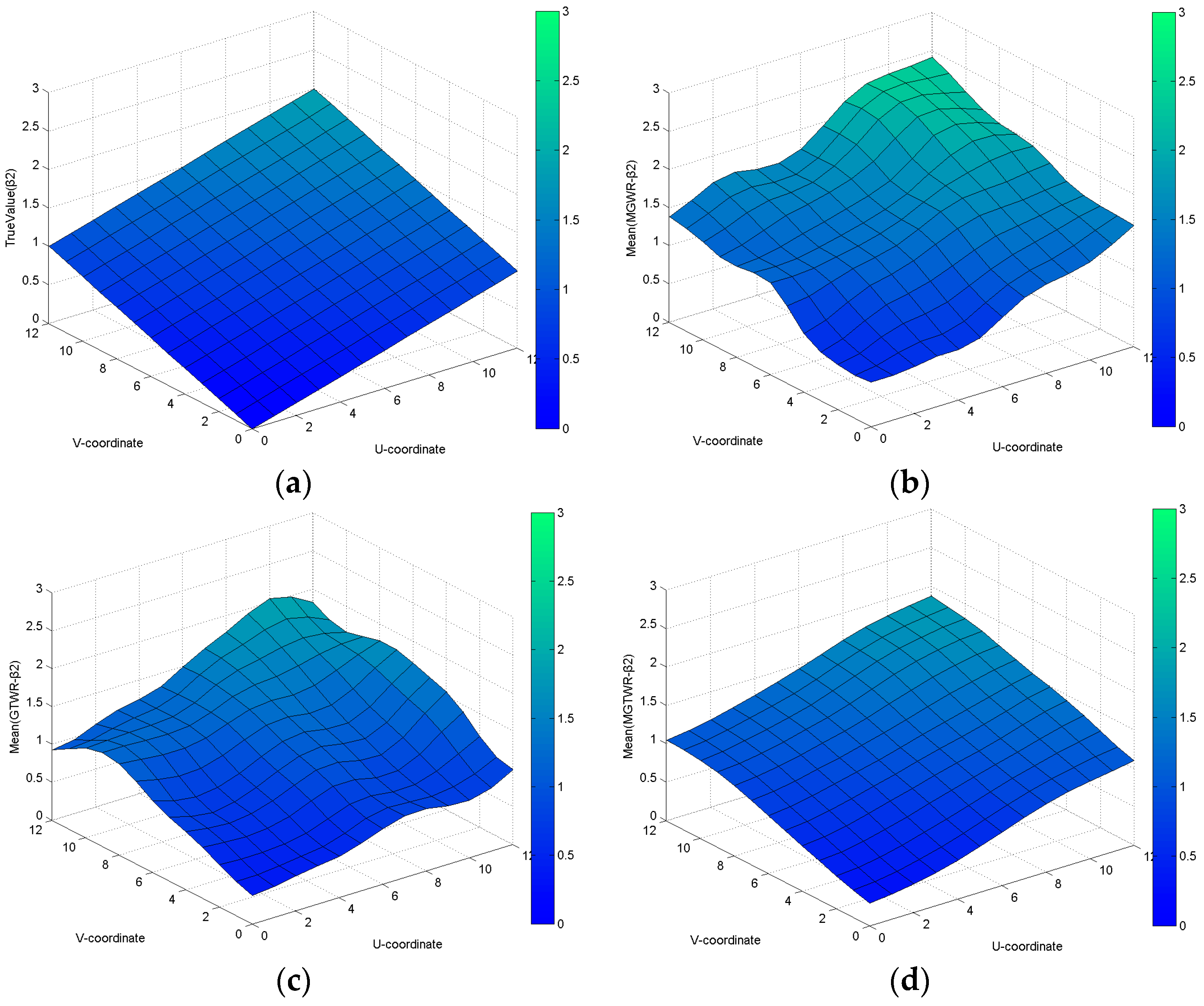Additionally, we designed Figure 6, Figure 7, Figure 8 and Figure 9 to illustrate the constant ${\mathsf{\beta }}_1$ and spatial-temporally varying coefficient ${\beta }_2$ in Dataset 3.

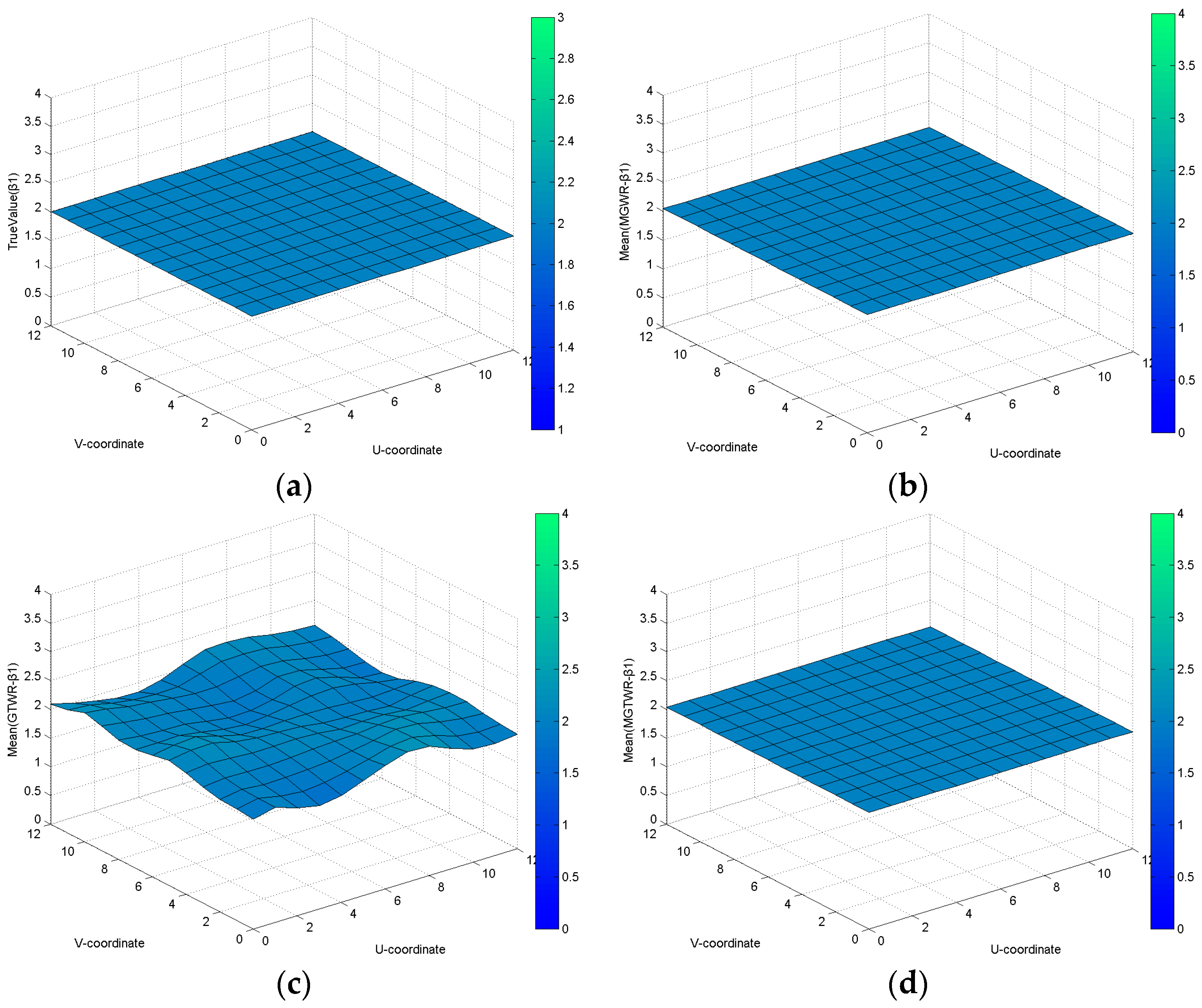
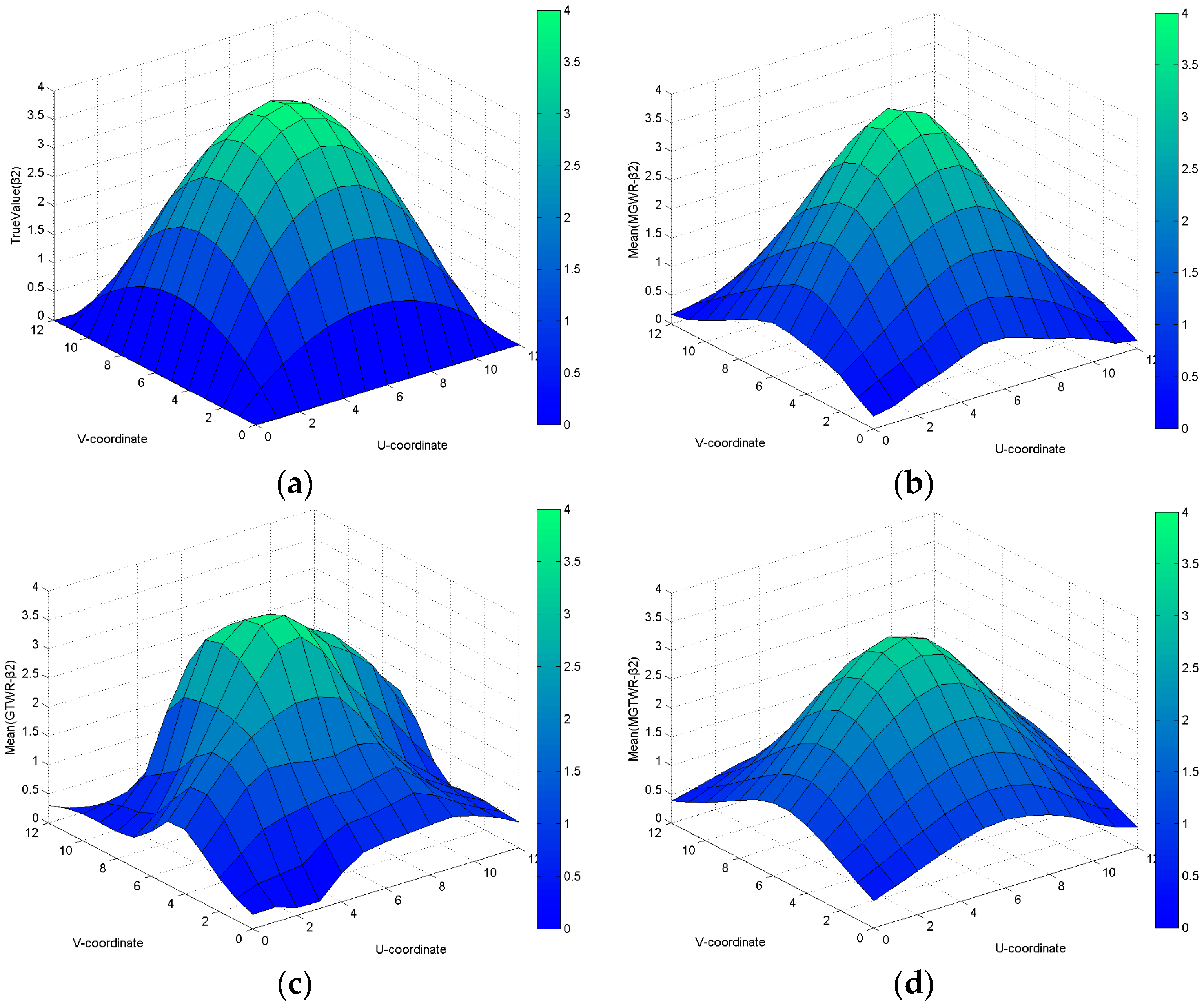
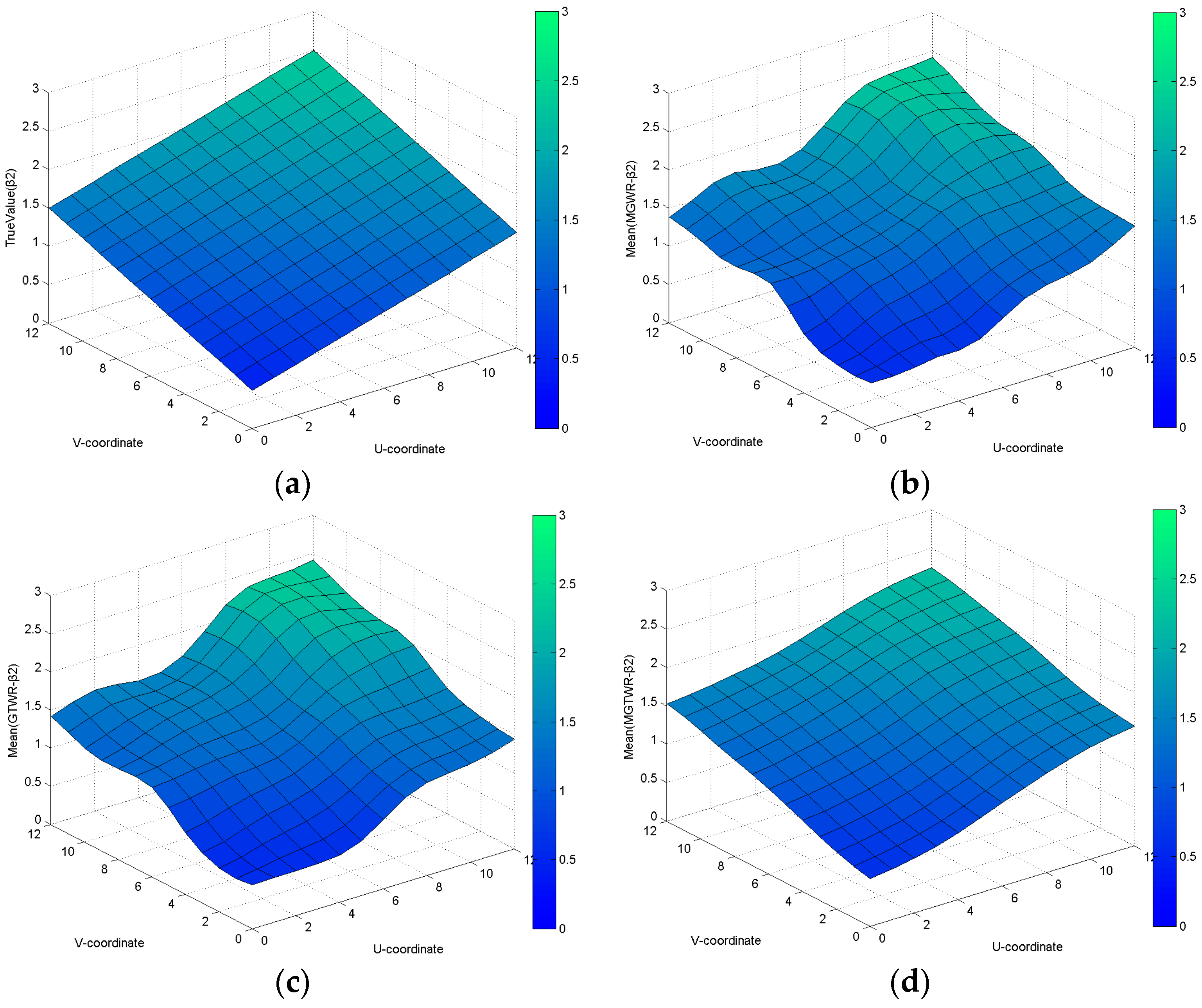
For the combinations of constant and spatially varying coefficients in Dataset 1, Table 2 shows that the AIC values of the MGWR, GTWR and MGTWR models are 592.1566, 635.0128 and 589.45, respectively. Compared to the MGWR and GTWR models, the improvements in the MGTWR model are 2.7066 and 45.5628, respectively. This change indicates that the MGTWR model achieved the best results. The estimated constant coefficient surfaces calculated using the MGWR and MGTWR models (Figure 1b,d, respectively) are smooth and similar to the true value, whereas the estimation constant coefficient surface calculated by the GTWR model (as shown in Figure 1c) greatly fluctuates from the true value.

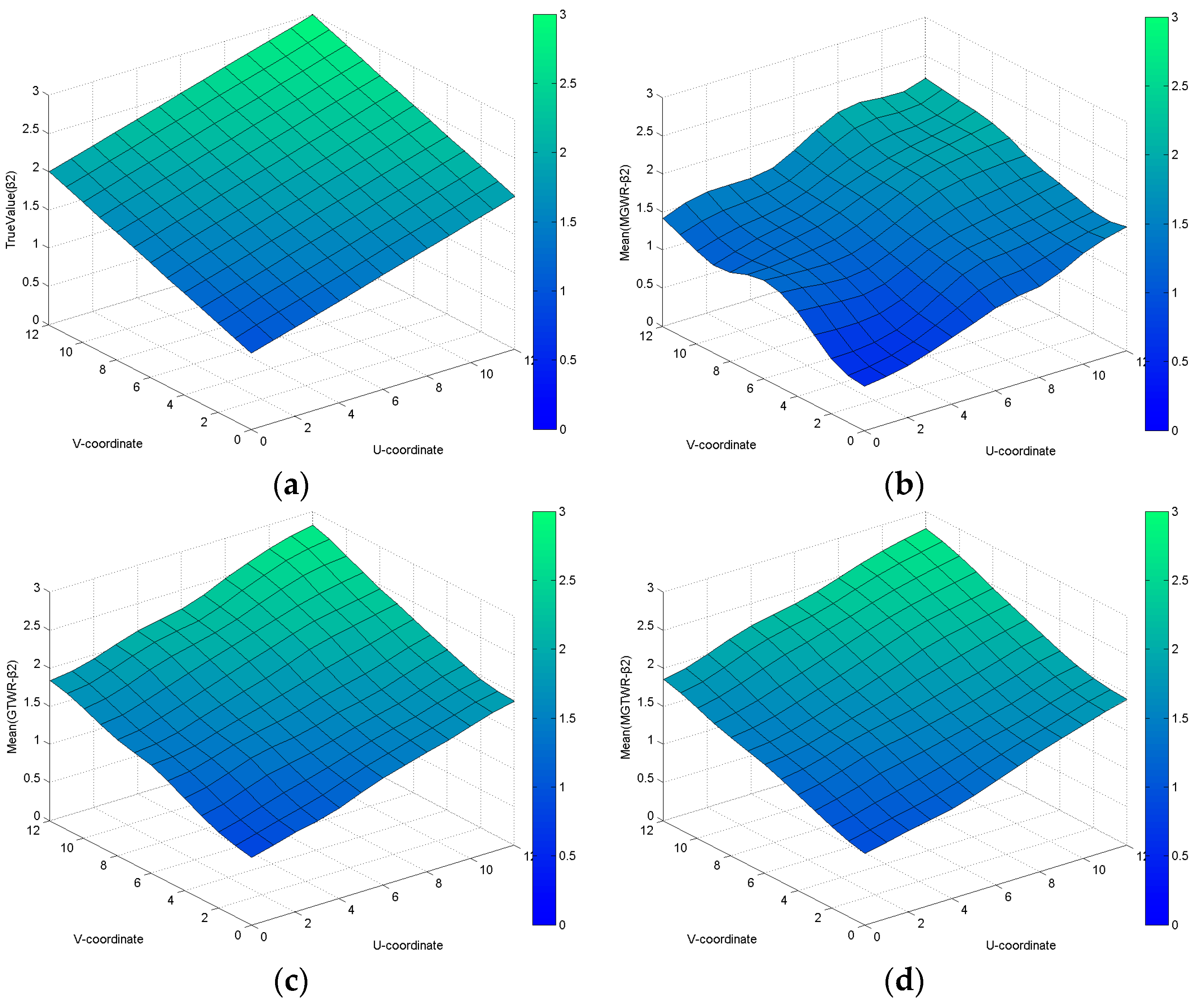
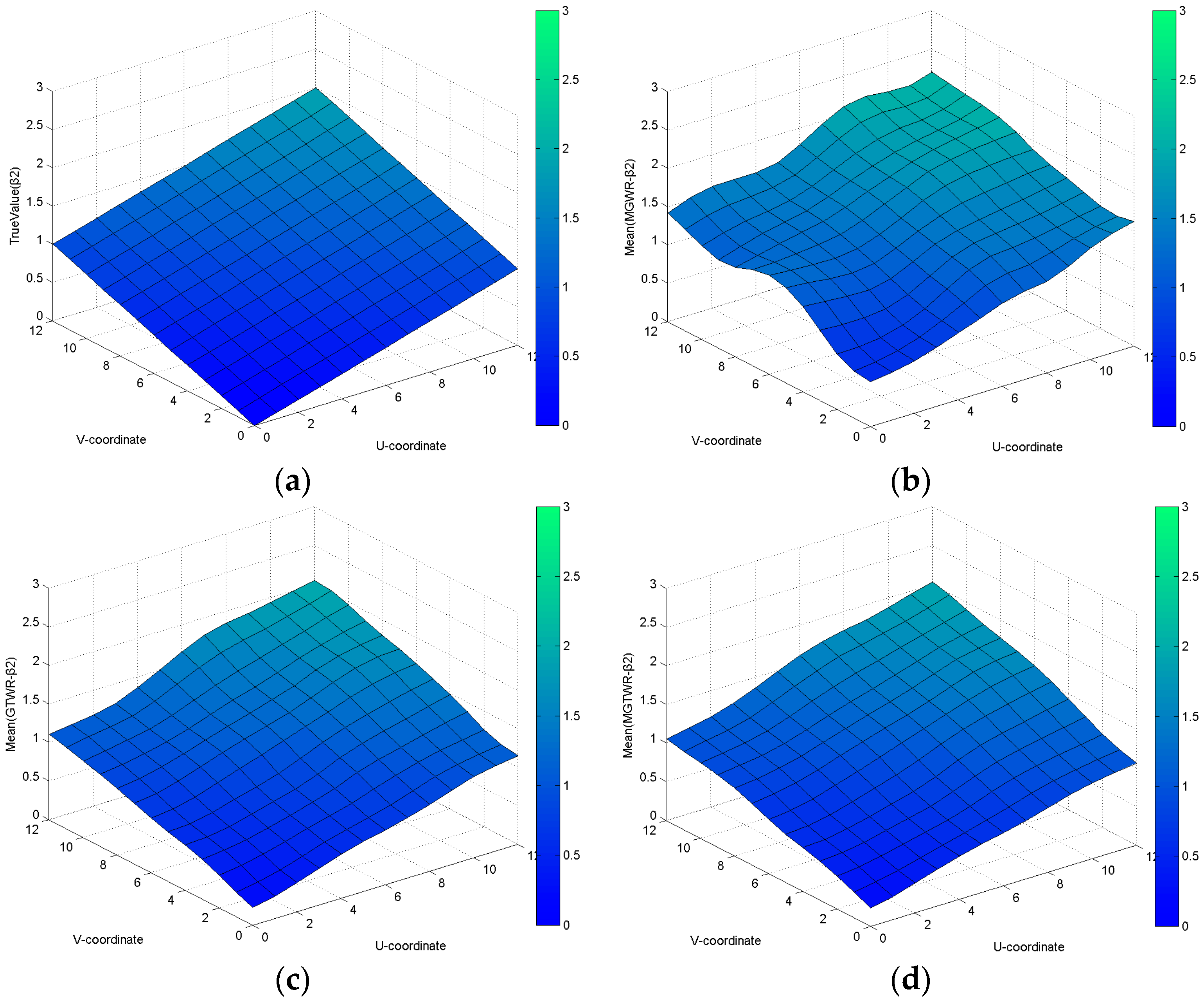
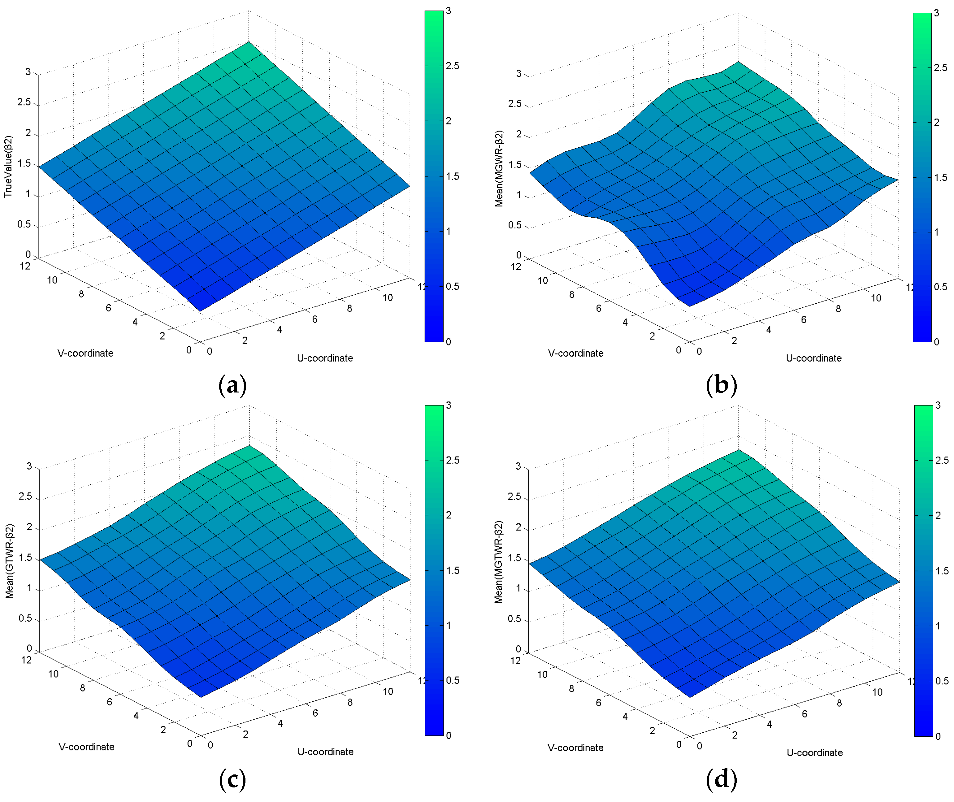
For the combinations of spatially and spatial-temporally varying coefficients in Dataset 2, the AIC values of the MGWR, GTWR and MGTWR models are 7168.606, 6493.464 and 6532.238, respectively, as shown in Table 2. Compared to the MGWR and GTWR models, the improvements in the MGTWR model are 36.368 and −38.774, respectively. These differences illustrate that the MGTWR model achieved the better performance. Figure 3, Figure 4 and Figure 5 present the distributions of spatial-temporally varying coefficients when t = 0, 6 and 12 in Dataset 2. The estimation coefficient surfaces calculated using the MGWR model are distributed between (0.5, 2.5) no matter how the temporal coordinate t changes. However, the estimated coefficient surfaces calculated using the GTWR and MGTWR models are distributed between (0, 2), (0.5, 2.5) and (1, 3) when t = 0, 6 and 12, respectively. Obviously, both the GTWR and MGTWR models can effectively simulate temporal variations.

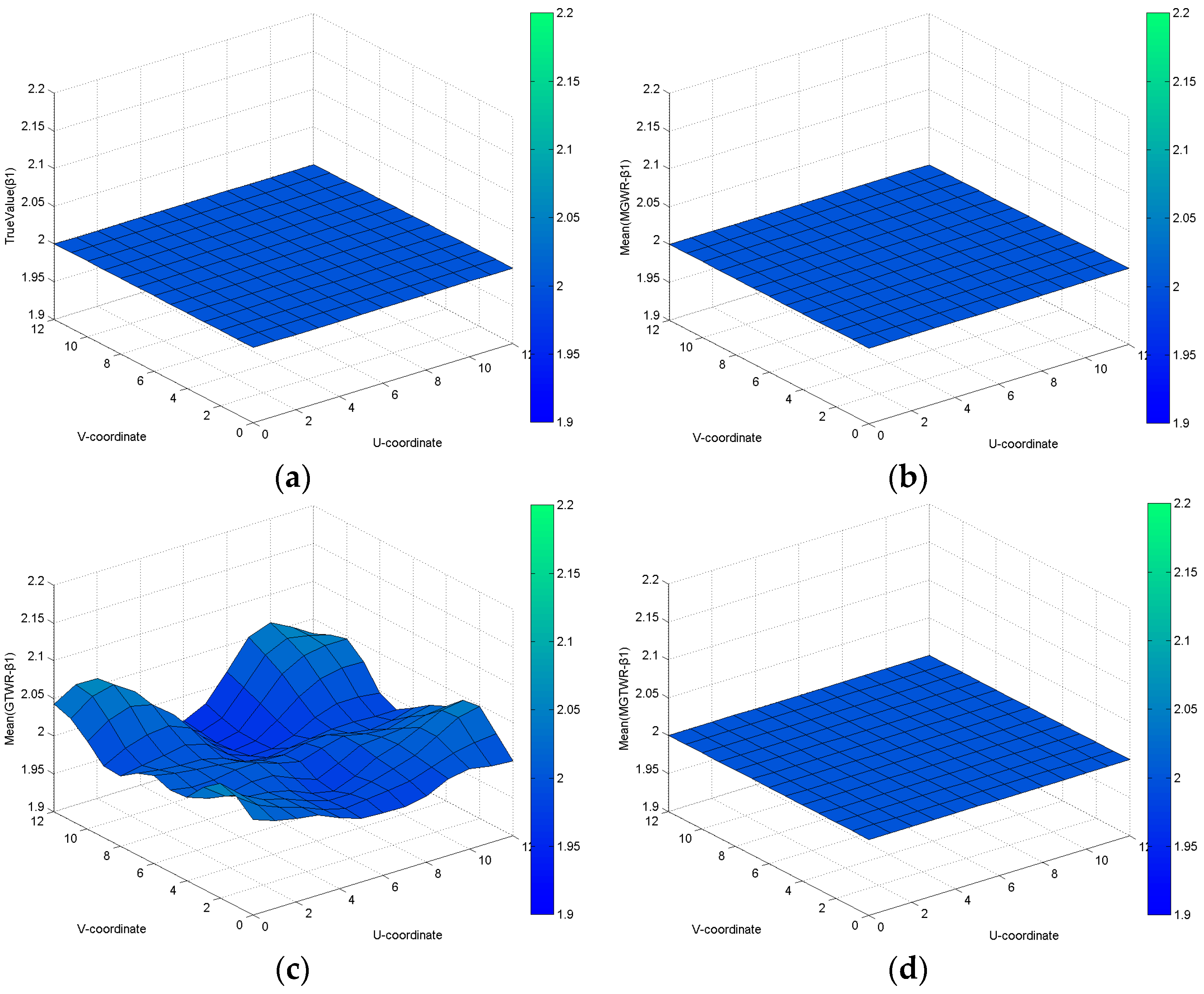
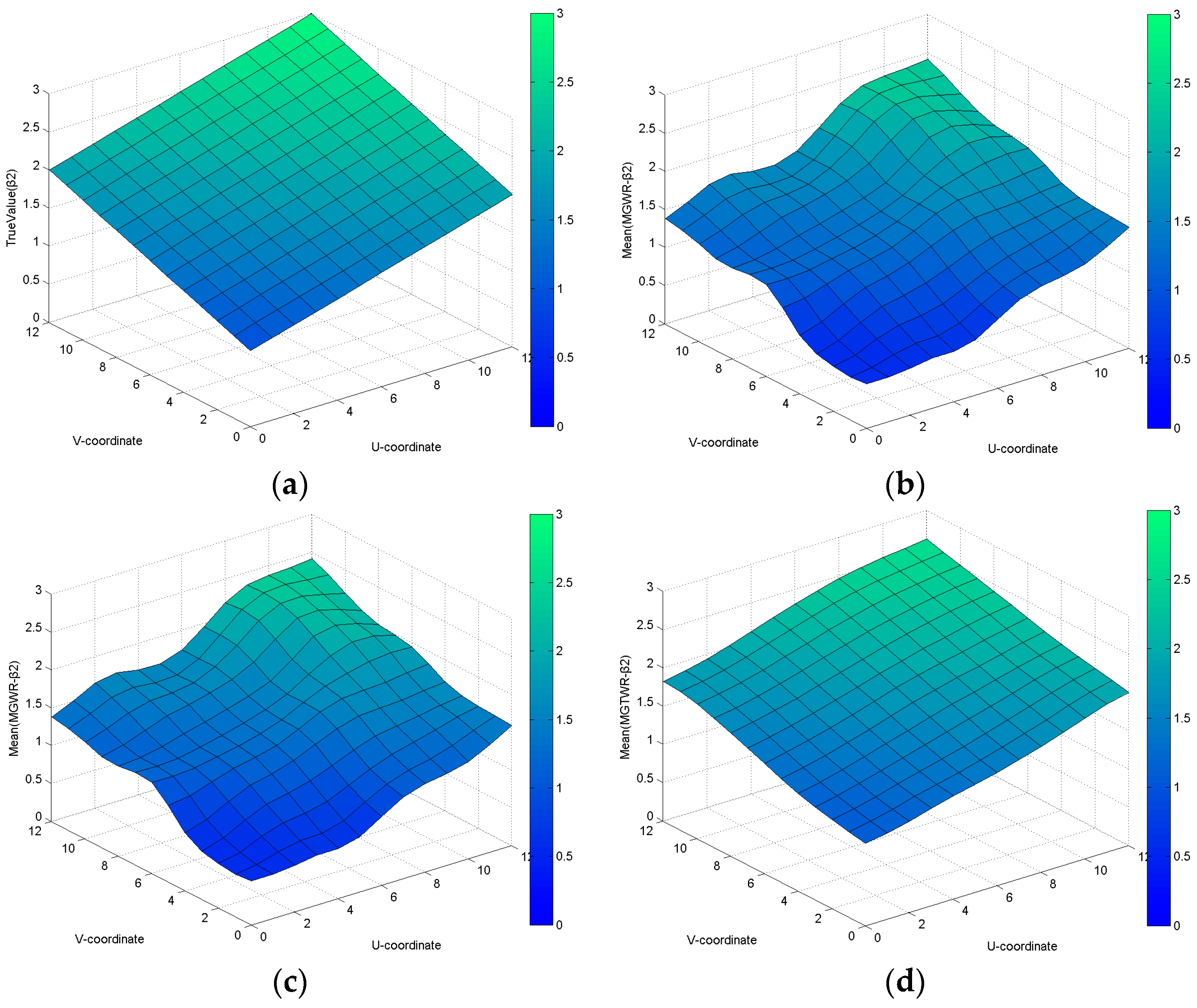
For combinations of constant coefficients and spatial-temporally varying coefficients in Dataset 3, the AIC values for the MGWR, GTWR and MGTWR models are 6516.37, 6439.214 and 6403.558, respectively. Additionally, the improvements in the MGTWR model compared to the GTWR and MGWR model are 112.812 and 35.656, respectively. The estimated coefficient surfaces for constant (Figure 6) and spatial-temporally varying coefficients (Figure 7, Figure 8 and Figure 9) reveal that the MGTWR model has superior efficiency in dealing with global stationarity and the local spatial-temporal non-stationarity problem.

3.2. The Real Data Experiments

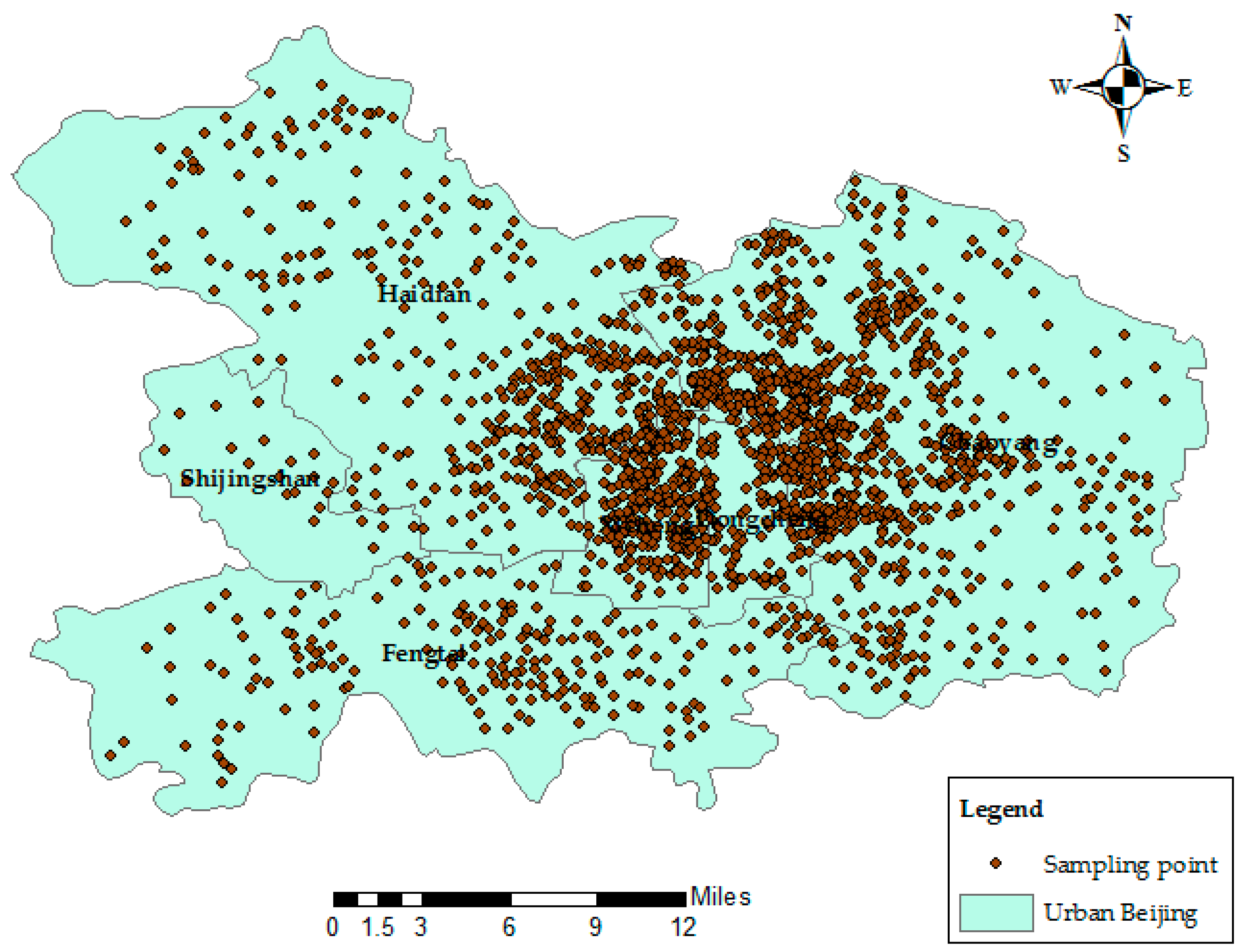
We tested the performance of the MGTWR model in the real world and established a hedonic price model of Beijing. The hedonic model examines the effects of characteristics of housing commodities on housing prices [29,30,31,32,33]. Such models regard houses as a composite commodity formed by structural attributes, neighborhood attributes, the age of construction and other attributes. The price of a property is assumed to be a realization of the value. The structural attributes include the housing area, the number of bedrooms, the residential plot ratio, the residential greening ratio and other factors. The neighborhood attributes include the influences of supermarkets, shopping centers, primary schools, gas stations and other factors. We obtained 1961 samples with attributes such as house price, house area, residential plot ratio, residential greening ratio, property management fee, the distance to the nearest primary school, the distance to the nearest shopping mall, age of construction and geographical coordinates [34]. The housing commodity data were provided by the National Bureau of Statistics, and Figure 10 illustrates the distribution of the housing commodity samples.

The description and units of the variables are shown in

Table 3. Descriptions and units of the variables used in the real data experiments.

Abbreviation	Description	Units
LnPrice	Residential sales price	RMB
LnPRatio	Log of the resident plot ratio	—
LnGRatio	Log of the resident greening ratio	—
LnFArea	Log of the housing area	Square meter
LnPFee	Log of the resident property management fee	RMB/Square meter
LnDpriSchool	Log of the distance to the nearest primary school	Meter
LnDShMall	Log of the distance to the nearest shopping mall	Meter
Age	Age of the building (with 1980 as the base year)	Year

. In Table 3, the dependent variable (LnPrice) is the logarithmically transformed sales price of the house in RMB units. The housing area is logarithmically transformed as LnFArea and is in units of m². The residential property management fee is logarithmically transformed as LnPFee and is in units of RMB/m². The distance to the nearest primary school is logarithmically transformed as LnD_priSchool and is in units of meters. The distance to the nearest shopping mall, also in units of meters, is logarithmically transformed as LnD_ShMall. Both the residential plot ratio and the residential greening ratio are logarithmically transformed as LnPRatio and LnGRatio. The temporal variable is the age of the building at the time of sale (Age) in units of years.

Before constructing the MGWR and MGTWR models to conduct the real data experiment, it was necessary to confirm which variables were stationary and which were non-stationary. We implemented a hypothesis test that assumed that all independent variables were non-stationary and established the F statistical (Leung et al. [35]) to detect the spatial and spatial-temporal variation in the coefficients [35,36]. Both the optimal bandwidth and spatial-temporal parameters required to calculate the F values were obtained using the CV method with a Gaussian kernel function. The results yielded an optimal spatial bandwidth of 7700 m and an optimal spatial-temporal parameter ratio of 1,500,000.

Table 4. The p-value of spatial-temporal non-stationary hypothesis test.

	Intercept	LnPRatio	LnGRatio	LnFArea	LnPFee	LnDpriSchool	LnDShMall	Age
Spatial	<0.001 *	>0.1	<0.001 *	<0.001 *	>0.3	<0.05 *	>0.1	<0.05 *
Spatial-temporal	<0.001 *	<0.001 *	<0.001 *	<0.001 *	>0.05	<0.001 *	<0.001 *	<0.001 *

* The statistically-significant values at the 5% level.

provides the p-value of spatial-temporal non-stationary hypothesis test and the statistically-significant values at the 5% level are marked with an asterisk “*”. The results illustrated that the residential plot ratio (LnPRatio), the property management fee (LnPFee) and the distance to the nearest shopping mall (LnD_ShMall) had nonsignificant spatial variations, and the remaining explanatory variables had significant spatial variations based on the spatial non-stationarity hypothesis test. Moreover, the property management fee (LnPFee) had non-significant spatial-temporal variations, and others had significant spatial-temporal variations based on the spatial-temporal non-stationarity test.

Based on the results of the spatial-temporal non-stationarity hypothesis test, we established the MGWR, GTWR and MGTWR models using the Gaussian kernel function in the real data experiment. In the MGWR model, the residential plot ratio (LnPRatio), the property management fee (LnPFee) and the distance to the nearest shopping mall (LnD_ShMall) were taken as constant variables. The remaining independent variables were taken as spatially varying variables. All the independent variables were taken as spatial-temporal variables in the GTWR model. Moreover, the property management fee (LnPFee) was taken as a constant variable in the MGTWR model, and the remaining independent variables were taken as spatial-temporal variables. CV criteria were used to calculate the optimal bandwidth and spatial-temporal parameters. The results showed that the optimal bandwidths of the MGWR, GTWR and MGTWR models were 8000 m, 7700 m, and 5080 m, respectively, and the optimal spatial-temporal parameter ratio of the GTWR and MGTWR models were 1,500,000 and 212,000, respectively. The leave-one-out cross-validation method was used to avoid overly optimistic results.

Table 5. Summaries of the estimation coefficients of the MGTWR model.

	Min	Lower Quartile	Mean	Median	Upper Quartile	Max	SD
Intercept	−6.5845	1.1898	1.6174	1.9083	2.2080	3.1061	0.9080
LnPRatio	−0.3655	−0.0126	0.0024	−0.0043	0.0084	0.2503	0.0294
LnGRatio	−2.0528	−0.1575	−0.0177	−0.0591	0.1127	2.1998	0.2201
LnFArea	−0.0487	0.8066	0.9286	0.942	1.0557	2.4133	0.1731
LnPFee	0.0223	0.0223	0.0223	0.0223	0.0223	0.0223	0.0000
LnDpriSchool	−0.0667	−0.0167	−0.0114	−0.0104	−0.0053	0.4763	0.0165
LnDShMall	−0.0901	0.0105	0.0241	0.0230	0.0380	0.6799	0.0291

provides summaries of the estimation coefficients of the MGTWR model, including the minimum (Min), lower quartile (LQ), mean (Mean), median (Median), upper quartile (UQ), maximum (Max) and standard deviation (SD). Additionally, diagnostic indices of the hedonic price model were adopted to examine the efficiency, similar method reported by Wo [17], i.e., we calculated the MSE, R², R²_adj and AIC values of the MGWR, GTWR and MGTWR models, as shown in

Table 6. Diagnostic information for the MGWR, GTWR, and MGTWR models.

	MSE	R2	R2adj	AIC
MGWR	0.0958	0.8135	0.8129	1113.1958
GTWR	0.078	0.8482	0.8477	987.7558
MGTWR	0.0691	0.8654	0.8649	858.9917
MGTWR/MGWR Improvement	27.87%	6.38%	6.40%	254.20
MGTWR/GTWR Improvement	11.41%	2.03%	2.03%	128.76

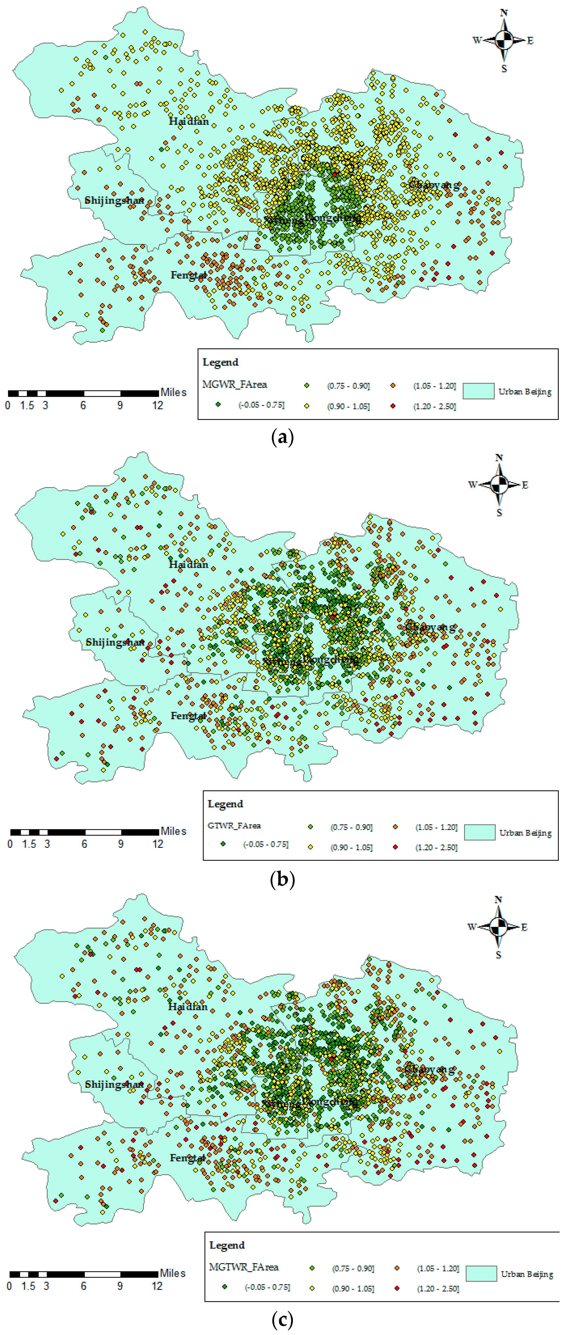
. In general, high R² and R²_adj values or low MSE and AIC values indicate a good fit between the different models and the sample data. An important characteristic of the MGWR, GTWR and MGTWR techniques is that the local relationships between estimated coefficients are mappable and visually analytic. Taking the estimated housing area coefficients as an example, we divided the value into five intervals and colored each interval to illustrate the spatial-temporal variation patterns, as shown in Figure 10.

As shown in Table 6, the mean squared errors of the MGWR, GTWR and MGTWR models were 0.0958, 0.078, and 0.0691, respectively. The MGTWR model yielded a 27.87% improvement over the MGWR and an 11.41% improvement over the GTWR model. Thus, the MGTWR exhibited the highest precision of all the models. Moreover, note that the goodness of fit increased from 0.8135 for the MGWR model to 0.8482 for the GTWR model and 0.8654 for the MGTWR model. Additionally, the AIC values of the MGTWR model decreased by 254.2 with respect to the MGWR model and by 128.76 with respect to the GTWR model.

3.3. Discussion

This paper proposes the MGTWR model and testes the efficiency of the MGWR, GTWR and MGTWR models under the following three conditions:

• Condition 1: global stationarity and spatial non-stationarity;
• Condition 2: spatial-temporal non-stationarity;
• Condition 3: global stationarity and spatial-temporal non-stationarity.

First, the MGTWR model is most applicable under Conditions 1 and 3. Under Condition 1, compared to the MGWR and GTWR models, the AIC value of the MGTWR model is reduced from 2.7066 (MGWR) to 45.5628 (GTWR) for Dataset 1. Under Condition 3, compared to the MGWR model, the AIC value of the MGTWR model is reduced by 112.812 (Dataset 3) and 254.20 (real data). Compared to the GTWR model, the AIC value of the MGTWR model is reduced by 35.656 (Dataset 3) and 128.76 (real data). Under Condition 2, the AIC value of the MGTWR model is reduced by 36.368 (MGWR) to −38.774 (GTWR) for Dataset 2. The results indicate that the MGTWR model is superior to the MGWR model but did not outperform the GTWR model. This phenomenon is caused by taking the spatial-temporal varying coefficients as constant coefficients in the MGTWR model, which leads to the result not remaining consistent with that of other conditions.

Second, from the perspective of the estimated spatial-temporal coefficients, the estimation coefficients of the MGTWR model are similar to the true values based on the simulated data (Figure 3, Figure 4 and Figure 5 and Figure 7, Figure 8 and Figure 9). In addition, as Figure 11 illustrates, the coefficients of the MGTWR (GTWR) models increase (decrease) sharply in Haidian District in the real data experiment compared to those of the MGWR model due to the spatial-temporal variations.

Third, from the perspective of the estimated constant coefficients, the estimated coefficients of the MGTWR and MGWR models are similar to the true values in the simulated data (Figure 1 and Figure 6). When the constants are treated as spatial-temporally varying coefficients, the estimation surface of the GTWR model shows a clear deviation from the true value (Figure 1c and Figure 6c). The real data experiment suggests that, although we can determine which coefficients are stationary and spatial-temporally non-stationary using the F statistic, the stationarity problem cannot be solved using the GTWR model. Therefore, we proposed a method that divides the explanatory variables into two groups, stationary and spatial-temporally non-stationary variables, and formulated a two-stage least squares estimation for the MGTWR model.

Finally, the real data experiment indicates that not all explanatory variables are spatially or spatial-temporally non-stationary. Under the 95% confidence level criterion, the property management fee (LnPFee) did not exhibit significant spatial-temporal or spatial variations, potentially because the growth rate of property management fees in the spatial-temporal or spatial dimension might be negligible compared to growth rate of the house price. This finding is evidence of the phenomenon that both global stationarity and spatial-temporal non-stationarity exist in the real word. Considering both the constant and spatial-temporally varying coefficients, the MGTWR model achieves more accurate estimation than do the MGWR or GTWR models.

4. Conclusions

Little attention has been given to the concept that both global stationarity and spatial-temporal non-stationarity exist. This paper proposed the MGTWR model, which divides the explanatory variables into stationary and spatial-temporal non-stationary variables, to complement the current literature regarding studies of geospatial regression. Furthermore, because the constant and spatial-temporal varying coefficients cannot be estimated in one step, the two-stage least squares estimation was introduced to calibrate the MGTWR model. Both simulation and real data experiments were conducted, and the performance of the MGTWR model was verified. Notably, it is important to explore spatial-temporal variations from global and local perspectives in the spatial modeling.

First, the experiment demonstrated that the MGTWR model had greater accuracy than the MGWR and GTWR models under conditions of stationarity and spatial-temporal non-stationarity. The constant and spatial-temporal estimation surfaces of the MGTWR model were almost consistent with the true values in the simulated data experiment. Second, the real data experiment proved the existence of both global stationarity and spatial-temporal non-stationarity, as well as the practical applicability of the proposed method. Finally, we demonstrated how to achieve the following goals using the MGTWR model: (i) develop a clear recognition of global and spatial-temporally varying coefficients; (ii) based on the above condition, establish the MGTWR model and calculate the fitting values of coefficients and dependent variables; and (iii) evaluate the efficiency of the MGTWR model using diagnostic indices.

Although we have performed numerous studies, some limitations should be addressed in further studies. During the experiment, we found the computational procedure of the MGTWR model to be computationally intensive and time consuming because of the size of the hat matrix. A further study will be performed to improve the computational performance by optimizing the complex weighting and hat matrixes.

References

1. Brunsdon, C.; Fotheringham, A.S.; Charlton, M.E. Geographically weighted regression: A method for exploring spatial nonstationarity. Geogr. Anal. 1996, 28, 281–298. [Google Scholar] [CrossRef]
2. Yin, J.; Gao, Y.; Du, Z.; Wang, S. Exploring multi-scale spatiotemporal twitter user mobility patterns with a visual-analytics approach. ISPRS Int. J. Geo-Inf. 2016, 5. [Google Scholar] [CrossRef]
3. Luan, H.; Quick, M.; Law, J. Analyzing local spatio-temporal patterns of police calls-for-service using Bayesian integrated nested laplace approximation. ISPRS Int. J. Geo-Inf. 2016, 5. [Google Scholar] [CrossRef]
4. Subasinghe, S.; Estoque, C.R.; Murayama, Y. Spatiotemporal analysis of urban growth using GIS and remote sensing: A case study of the Colombo metropolitan area, Sri Lanka. ISPRS Int. J. Geo-Inf. 2016, 5. [Google Scholar] [CrossRef]
5. Brunsdon, C.; Fotheringham, A.S.; Charlton, M. Some notes on parametric significance tests for geographically weighted regression. J. Reg. Sci. 1999, 39, 497–524. [Google Scholar] [CrossRef]
6. Fotheringham, A.S.; Brunsdon, C.; Charlton, M. Geographically Weighted Regression; Wiley: Chichester, UK, 2002. [Google Scholar]
7. Wang, N.; Mei, C.-L.; Yan, X.-D. Local linear estimation of spatially varying coefficient models: An improvement on the geographically weighted regression technique. Environ. Plan. A 2008, 40, 986–1005. [Google Scholar] [CrossRef]
8. Cho, S.; Lambert, D.M.; Kim, S.G.; Jung, S. Extreme coefficients in geographically weighted regression and their effects on mapping. GISci. Remote Sens. 2009, 46, 273–288. [Google Scholar] [CrossRef]
9. Song, W.; Jia, H.; Huang, J.; Zhang, Y. A satellite-based geographically weighted regression model for regional PM2.5 estimation over the Pearl River Delta region in China. Remote Sens. Environ. 2014, 154, 1–7. [Google Scholar] [CrossRef]
10. You, W.; Zang, Z.; Zhang, L.; Li, Y.; Pan, X.; Wang, W. National-scale estimates of ground-level PM2.5 concentration in China using geographically weighted regression based on 3 km resolution MODIS AOD. Remote Sens. 2016, 8, 184. [Google Scholar] [CrossRef]
11. Wheeler, D.; Tiefelsdorf, M. Multicollinearity and correlation among local regression coefficients in geographically weighted regression. J. Geogr. Syst. 2005, 7, 161–187. [Google Scholar] [CrossRef]
12. Zhang, H.; Mei, C. Local least absolute deviation estimation of spatially varying coefficient models: Robust geographically weighted regression approaches. Int. J. Geogr. Inf. Sci. 2011, 25, 1467–1489. [Google Scholar] [CrossRef]
13. Harris, R.; Dong, G.; Zhang, W. Using contextualized geographically weighted regression to model the spatial heterogeneity of land prices in Beijing, China. Trans. GIS 2013, 17, 901–919. [Google Scholar] [CrossRef]
14. Lu, B.; Charlton, M.; Harris, P.; Fotheringham, A.S. Geographically weighted regression with a non-Euclidean distance metric: A case study using hedonic house price data. Int. J. Geogr. Inf. Sci. 2014, 28, 660–681. [Google Scholar] [CrossRef]
15. Lu, B.; Charlton, M.; Brunsdon, C.; Harris, P. The Minkowski approach for choosing the distance metric in geographically weighted regression. Int. J. Geogr. Inf. Sci. 2016, 30, 351–368. [Google Scholar] [CrossRef]
16. Huang, B.; Wu, B.; Barry, M. Geographically and temporally weighted regression for modeling spatio-temporal variation in house prices. Int. J. Geogr. Inf. Sci. 2010, 24, 383–401. [Google Scholar] [CrossRef]
17. Wu, B.; Li, R.; Huang, B. A geographically and temporally weighted autoregressive model with application to housing prices. Int. J. Geogr. Inf. Sci. 2014, 28, 1186–1204. [Google Scholar] [CrossRef]
18. Yu, D. Understanding regional development mechanisms in greater Beijing area, China, 1995–2001, from a spatial–temporal perspective. GeoJournal 2014, 79, 195–207. [Google Scholar] [CrossRef]
19. Chu, H.-J.; Huang, B.; Lin, C.-Y. Modeling the spatio-temporal heterogeneity in the PM10-PM2.5 relationship. Atmos. Environ. 2015, 102, 176–182. [Google Scholar] [CrossRef]
20. Bai, Y.; Wu, L.; Qin, K.; Zhang, Y.; Shen, Y.; Zhou, Y. A geographically and temporally weighted regression model for ground-level PM2.5 estimation from satellite-derived 500 m resolution AOD. Remote Sens. 2016, 8, 262. [Google Scholar] [CrossRef]
21. Wrenn, D.H.; Sam, A.G. Geographically and temporally weighted likelihood regression: Exploring the spatiotemporal determinants of land use change. Reg. Sci. Urban Econ. 2014, 44, 60–74. [Google Scholar] [CrossRef]
22. Fotheringham, A.S.; Crespo, R.; Yao, J. Geographical and temporal weighted regression (GTWR). Geogr. Anal. 2015, 47, 431–452. [Google Scholar] [CrossRef]
23. Mei, C.-L.; He, S.-Y.; Fang, K.-T. A note on the mixed geographically weighted regression model. J. Reg. Sci. 2004, 44, 143–157. [Google Scholar] [CrossRef]
24. Wei, C.-H.; Qi, F. On the estimation and testing of mixed geographically weighted regression models. Econ. Model. 2012, 29, 2615–2620. [Google Scholar] [CrossRef]
25. Kang, D.; Dall’erba, S. Exploring the spatially varying innovation capacity of the US counties in the framework of Griliches’ knowledge production function: A mixed GWR approach. J. Geogr. Syst. 2016, 18, 125–157. [Google Scholar] [CrossRef]
26. Badinger, H.; Egger, P. Fixed effects and random effects estimation of higher-order spatial autoregressive models with spatial autoregressive and heteroscedastic disturbances. Spat. Econ. Anal. 2014, 10, 11–35. [Google Scholar] [CrossRef] [Green Version]
27. Akaike, H. Information Theory and an Extension of the Maximum Likelihood Principle. In Proceedings of the second International Symposium on Information Theory, Tsahkadsor, Armenia, 2–8 September 1971; pp. 267–281.
28. Hurvich, C.M.; Simonoff, J.S.; Tsai, C.-L. Smoothing parameter selection in nonparametric regression using an improved Akaike information criterion. J. R. Stat. Soc. Ser. B 1998, 60, 271–293. [Google Scholar] [CrossRef]
29. Páez, A.; Long, F.; Farber, S. Moving window approaches for hedonic price estimation: An empirical comparison of modelling techniques. Urban Stud. 2008, 45, 1565–1581. [Google Scholar] [CrossRef]
30. Peterson, S.; Flanagan, A. Neural Network Hedonic Pricing Models in Mass Real Estate Appraisal. J. Real Estate Res. 2009. Available online: https://papers.ssrn.com/sol3/papers.cfm?abstract_id=1086702 (accessed on 24 January 2017). [Google Scholar]
31. Kuşan, H.; Aytekin, O.; Özdemir, İ. The use of fuzzy logic in predicting house selling price. Expert Syst. Appl. 2010, 37, 1808–1813. [Google Scholar] [CrossRef]
32. Selim, S. Determinants of house prices in Turkey: A hedonic regression model. Doğuş Üniversitesi Dergisi 2011, 9, 65–76. [Google Scholar]
33. Helbich, M.; Brunauer, W.; Vaz, E.; Nijkamp, P. Spatial heterogeneity in hedonic house price models: The case of Austria. Urban Stud. 2013, 51, 390–411. [Google Scholar] [CrossRef]
34. Liu, J.; Yang, Y.; Xu, S. A geographically temporal weighted regression approach with travel distance for house price estimation. Entropy 2016, 18, 303. [Google Scholar] [CrossRef]
35. Leung, Y.; Mei, C.L.; Zhang, W.X. Statistical tests for spatial nonstationarity based on the geographically weighted regression model. Environ. Plan. A 2000, 32, 9–32. [Google Scholar] [CrossRef]
36. Xuan, H.; Li, S.; Amin, M. Statistical inference of geographically and temporally weighted regression model. Pak. J. Stat. 2015, 31, 307–325. [Google Scholar]
Figure 1. Dataset 1: Visualization of the simulated and fitted coefficient β 1 . (a) The true value; (b) The mean value calculated by MGWR; (c) The mean value calculated by GTWR; (d) The mean value calculated by MGTWR.
Entropy 19 00053 g001
Figure 2. Dataset 1: Visualization of the simulated and fitted coefficient β 2 . (a) The true value; (b) The mean value calculated by MGWR; (c) The mean value calculated by GTWR; (d) The mean value calculated by MGTWR.
Entropy 19 00053 g002
Figure 3. Dataset 2: Visualization of the simulated and fitted coefficient β 2 at t = 0. (a) The true value; (b) The mean value calculated by MGWR; (c) The mean value calculated by GTWR; (d) The mean value calculated by MGTWR.
Entropy 19 00053 g003
Figure 4. Dataset 2: Visualization of the simulated and fitted coefficient β 2 at t = 6. (a) The true value; (b) The mean value calculated by MGWR; (c) The mean value calculated by GTWR; (d) The mean value calculated by MGTWR.
Entropy 19 00053 g004
Figure 5. Dataset 2: Visualization of the simulated and fitted coefficient β 2 at t = 12. (a) The true value; (b) The mean value calculated by MGWR; (c) The mean value calculated by GTWR; (d) The mean value calculated by MGTWR.
Entropy 19 00053 g005
Figure 6. Dataset 3: Visualization of the simulated and fitted coefficient β 1 . (a) The true value; (b) The mean value calculated by MGWR; (c) The mean value calculated by GTWR; (d) The mean value calculated by MGTWR.
Entropy 19 00053 g006
Figure 7. Dataset 3: Visualization of the simulated and fitted coefficient β 2 at t = 0. (a) The true value; (b) The mean value calculated by MGWR; (c) The mean value calculated by GTWR; (d) The mean value calculated by MGTWR.
Entropy 19 00053 g007
Figure 8. Dataset 3: Visualization of the simulated and fitted coefficient β 2 at t = 6. (a) The true value; (b) The mean value calculated by MGWR; (c) The mean value calculated by GTWR; (d) The mean value calculated by MGTWR.
Entropy 19 00053 g008
Figure 9. Dataset 3: Visualization of the simulated and fitted coefficient β 2 at t = 12. (a) The true value; (b) The mean value calculated by MGWR; (c) The mean value calculated by GTWR; (d) The mean value calculated by MGTWR.
Entropy 19 00053 g009
Figure 10. The distribution of housing commodity samples in urban Beijing.
Entropy 19 00053 g010
Figure 11. The regression coefficients of the housing areas of different models. (a) The housing area regression coefficients of the MGWR model; (b) The housing area regression coefficients of the GTWR model; (c) The housing area regression coefficients of the MGTWR model.
Entropy 19 00053 g011