Information Geometric Approach to Recursive Update in Nonlinear Filtering

Abstract

The measurement update stage in the nonlinear filtering is considered in the viewpoint of information geometry, and the filtered state is considered as an optimization estimation in parameter space has been corresponded with the iteration in the statistical manifold, then a recursive method is proposed in this paper. This method is derived based on the natural gradient descent on the statistical manifold, which constructed by the posterior probability density function (PDF) of state conditional on the measurement. The derivation procedure is processing in the geometric viewpoint, and gives a geometric interpretation for the iteration update. Besides, the proposed method can be seen as an extended for the Kalman filter and its variants. For the one step in our proposed method, it is identical to the Extended Kalman filter (EKF) in the nonlinear case, while traditional Kalman filter in the linear case. Benefited from the natural gradient descent used in the update stage, our proposed method performs better than the existing methods, and the results have showed in the numerical experiments.

1. Introduction

Nonlinear filtering is a significant issue in the field of signal processing, such as target tracking, navigation and audio signal processing. However, there is no close form solution for nonlinear filtering similar to the Kalman filter for linear and Gaussian scenarios. How to deal with the nonlinear state propagation or nonlinear measurement is crucial in the research of nonlinear filtering. Various nonlinear filtering algorithms have been proposed and widely used in the practical applications, such as Extended Kalman filter (EKF) [1], Unscented Kalman filter (UKF) [2], Cubature Kalman filter (CKF) [3], and Particle filter (PF) [4]. Among these methods, EKF, UKF and CKF can be classified into the same catalog, which also has been called as KF-type method that have the certain nonlinear approximation to utilize the common frame of traditional Kalman filter to achieve the goal. Some relations among these KF-type method are given in [5]. The EKF utilizes the Taylor Series Expansion to exploit the analytical structure of nonlinear functions, which also be called as analytical linearization. Similarly, the UKF or CKF which exploit the statistical properties of Gaussian variables that undergo nonlinear transformations, which known as statistical linearization. While the PF is another catalog, which uses the Monte Carlo technique to approximate the PDF. It obtains a weighted sample from the posterior PDF, and provides an asymptotically exact approximation of the posterior PDF as the sample size tends to infinity [6]. In particular, all of these methods can be unified in the framework of Bayesian filtering [7] to induce the optimal estimation of state by means of computing the posterior PDF, i.e., the density of state conditional on the corresponding measurements.

As for the Bayesian filtering, the procedure can be split into two steps: time propagation and measurement update, which also have been called prediction and correction steps in same articles. In the nonlinear and non-Gaussian case, the state propagation step is relatively simple as it can be obtained by approximating the first two moments of the state variable that undergoes a transformation along the state transition function. But the measurement update is more difficult and challenging. Firstly, the measurement is proceeded not easily in itself, with nonlinear and/or non-Gaussian conditions. Secondly, the error which brings by the approximation of state propagation becomes more seriously under the nonlinear measurements. Thirdly, the measurement update step has associated state with measurement, and the posterior PDF of state has to be computed conditional on the measurement with noisy. Therefore, the posterior PDF is the key way to tackle this issue, and it attracted extensive attention in the research. Usually, Gaussian approximation to posterior PDF is used in the measurement update because of the analytically intractable in non-Gaussian scenario [8]. There are two most popular estimators being utilized in the estimation for posterior PDF as the criterion. The one is the linear minimum mean square error (LMMSE) estimator, which approximates the posterior mean and covariance matrix by its estimator and its mean square error matrix, respectively. Based on the LMMSE, Zanetti [9,10] proposes a recursive update method for the measurement update, which overcomes some of the limitations of the EKF. In addition, the famous methods, such as EKF, UKF and CKF can be classified in this class [11]. Another is the maximum a posteriori (MAP) estimator, which estimates the posterior mean and obtain the covariance matrix by linearizing the measurement function around the MAP estimate. As the most well-known iterated EKF (IEKF), which based on the Gauss-Newton optimization [12] or Levenberg-Marquardt (LM) method [13], is categorized in this class. Usually, these iterative methods for nonlinear filter have the better performance. As Lefebvre [14] has shown that IEKF outperform the EKF, unscented Kalman filter (UKF) for implementing the measurement update of the covariance matrix. Besides, there are some other methods to analysis and approximate the posterior PDF recently, such as the Kullback-Leibler divergence (KLD) as metric to analysis the performance from the true joint posterior PDF of the state conditional on the measurement to approximation posterior PDF [15]. This metric can be used to devise new algorithms, such as the iterated posterior linearization filter (IPLF) [8] which can be seen as an approximate recursive KLD minimization procedure.

In particular, when we consider the posterior PDF parameterized by the estimators in itself, some natural characters may attract our attentions and provides a new viewpoints on the estimation. During the posterior PDF approximated recursively by the MAP estimator, a family of the posterior PDFs parameterized by the estimators can construct a statistical manifold, which a Riemannian manifold of probability distributions. Thus, the better approximation of the true posterior PDF can be viewed as the search for the optimum in the statistical manifold. Usually, the search along the direction of conventional gradient can obtain the optimum with the faster speed and better convergence in Euclidean space, but not for the statistical manifold. For the sake of utilizing gradient in statistical manifold, Amari [16,17] has proposed the natural gradient descent for the search direction traditionally motivated from the perspective of information geometry, and it has been proved that steps along the direction of natural gradient descent is the steepest descent in the Riemannian manifold [18]. Based on the direction of steepest descent, the natural gradient descent can obtain the optimum in manifold with faster speed and better convergence. Because of these properties, it has been acted a new tool to analysis the nonlinear in the statistical problems with an optimization perspective. Further, it provides some geometric information, such as Riemannian metrics, distances, curvature and affine connections [19], which may be improve the performance of estimation. To characterize this geometric information, there are two important elements should be considered. The one is that considering the set of PDF as a statistical manifold, and another is the Fisher Information Matrix as the metric of the statistical manifold. With the defining metric by information geometry, the natural gradient descent can be constructed as the product of inverse of Fisher Matric and the conventional steepest. After it has been proposed, natural gradient descent works well for many applications as an alternative to stochastic gradient descent, such as neural network [20,21], Blind Separation [22], evolution strategy [23,24], and stochastic distribution control systems [25].

Motivated by the recursively estimation for nonlinear measurement update in the Bayesian filtering, we propose a method by using the natural gradient descent method in the statistical manifold constructed by the posterior PDF for measurement update in the nonlinear filtering. After the procedure of the state propagation, the prediction state can be as a prior information in the Bayesian framework. The statistical manifold will be constructed by the posterior PDF. We consider a geometric structure of a this manifold equipped with the Fisher metric, and construct an alternate recursive process on the manifold. Given an initial point in the manifold based on the prior information, the iterated method to seek the optimum can been achieved along the natural gradient steepest descent. At each iteration, the algorithm moves from the current estimate to a new estimate along the geodesic in the direction of the natural gradient descent with a step size. Our method has the better performance compared with the update of EKF, which occur an overshooting in some nonlinear case. In addition, it has also given the theoretical justification for the nonlinear measurement update in the filtering from the information geometry insight and a mathematical interpretation of this method. There are two advantages in the estimation procedure benefitting from the natural gradient descent method. Firstly, based on the fact that the Fisher information matrix (FIM) is the inverse of Cramer-Rao Limit Bounds(CRLB) with respect to the estimation, the natural gradient descent, which has used FIM as metric in the statistical manifold, may achieve the better performance of estimation. Secondly, the natural gradient descent is asymptotically Fisher efficient and often converges faster than the conventional gradient descent shown in [16]. With the better performance and fast convergence, the measurement update with natural gradient descent may be achieved better and faster. Furthermore, based on this measurement update stage, we can construct the different nonlinear filtering method with different state prediction method.

The paper is organized as follows. In Section 2, we give a description for estimation in the statistical manifold and derive the iteration estimation procedure in the viewpoint of information geometry. Then the measurement update using natural gradient descent has deduced in the Section 3. The differences between our proposed method and other existing methods have be discussed in the Section 4. In Section 5, the numerical experiments are presented to illustrate the performance compared with other existing methods. Finally, conclusions are made in Section 6.

2. Information Geometry and Natural Gradient Descent

Information geometry [17] is a new mathematical tool for the study of manifolds of probability distributions. It opens a new prospective to study the geometric structure of information theory and provides a new way to deal with existing statistical problems. It has the powerful ability to handle the non-Gaussian PDF case, such as Weibull distributions [19,26], gamma distributions [27], multivariate generalized Gaussian distribution [28], and non-Euclidean case, for example, the statistical manifold [29], the morphogenetic system [30]. For the optimization problems in statistical signal processing, the Natural gradient descent traditionally motivated from the perspective of information geometry and gradient descent method, has become an alternative to recursive estimation in the statistical manifold. It has a better performance and faster convergence.

Usually in the Euclidean space, the recursive method for estimation can be along the direction of steepest descent in which is relatively straightforward, but it is not the straightforward direction in the Riemannian geometry because of the curved coordinate system. In this case, the curvature of the manifold should be considered, and the steepest gradient descent should follow the curvature of the manifold. This is the important factor for estimation in the manifold, which has been considered in the natural gradient descent method.

In the view of information geometry, the initial point and the target point in the Riemannian manifold are corresponding with the initial and final estimation in the parameters space, respectively. Thus the estimation of parameters can be converted to the recursive procedure seeking optimum in the manifold. With the direction provided by the natural gradient descent, the recursive in the Riemannian manifold can obtain the optimization estimation of parameters.

In a Riemannian manifold, the Riemannian metric $g_p$ is used at every point p, which describes the relationship between the tangent space and its neighborhood tangent space. If the tangent vectors at point p base on the basis $v_p^1,...,v_p^n$ , then the Riemannian metric can be obtained as $g_p^{ij}=\langle v_p^i,v_p^j\rangle$, where $\langle ·,·\rangle$ denotes an inner product defined on the tangent space as the same as in the Euclidean space. With these definitions, the inner product of tangent space at point p can be induced as ${\langle w_p,w_q\rangle }_g=w_p^{\mathrm{T}}g{w}_q$, where $w_p\in T_p\mathcal{M}$ and $w_q\in T_p\mathcal{M}$. Given the description of tangent basis $w_p={\sum }_{i=1}^n{\alpha }_i{v}_p^i$ and $w_q={\sum }_{j=1}^n{\beta }_j{v}_p^j$, their inner product will be ${\langle w_p,w_q\rangle }_g={\sum }_{i,j=1}^n{g}_p^{ij}{\alpha }_i{\beta }_j$.

Consider a family of probability distributions $\mathcal{S}$ on ${\mathbb{R}}^d$ parameterized by n real-valued variables $\theta ={[{\theta }_1\cdots {\theta }_n]}^{\mathrm{T}}$ as

$$\begin{array}{c}\hfill \mathcal{S}=\{p_{\theta }=p\left(y;\theta \right)|\theta \in \Theta \}\end{array}$$

(1)

where $y\in {\mathbb{R}}^d$ is a random variable and Θ is a open subset of ${\mathbb{R}}^n$. The mapping $\phi :\mathit{S}\to {\mathbb{R}}^n$ defined by $\phi \left(p_{\theta }\right)=\theta$ can be viewed as a coordinate system of $\mathcal{S}$. With the Fisher information matrix (FIM)

$$\begin{array}{c}\hfill \mathbf{F}\left(\theta \right)=\int \frac{\partial logp\left(y;\theta \right)}{\partial \theta }{\left(\frac{\partial logp\left(y;\theta \right)}{\partial \theta }\right)}^{\mathrm{T}}p\left(y;\theta \right)dy\end{array}$$

(2)

as the Riemannian metric $\mathbf{G}\left(\theta \right)$ in the view of information geometry, which also termed Fisher metric, the $\mathcal{S}$ can be considered as a Riemannian manifold. Thus the $\mathcal{S}$ can be called an n-dimensional statistical manifold on ${\mathbb{R}}^d$, which the parameter θ plays the role of the coordinate system for $\mathcal{S}$. The element of the Riemannian metric $\mathbf{G}\left(\theta \right)=\left[{\mathit{g}}_{ij}\left(\theta \right)\right]$ can be written as the follow formation

$$\begin{array}{c}\hfill {\mathit{g}}_{ij}\left(\theta \right)=\mathbf{E}\left[\frac{\partial logp\left(y;\theta \right)}{\partial {\theta }_i}\frac{\partial logp\left(y;\theta \right)}{\partial {\theta }_j}\right]\end{array}$$

(3)

where $\mathbf{E}$ denotes the expectation with respect to y. The Fisher metric is the only invariant metric to be given to the statistical manifold [31]. Because of the fact that

$$\begin{array}{cc}\hfill \mathbf{E}\left[\frac{\partial logp\left(y;\theta \right)}{\partial {\theta }_i}\right]& =\int \frac{\partial logp\left(y;\theta \right)}{\partial \theta }p\left(y;\theta \right)dy\hfill \\ & =\frac{\partial }{\partial \theta }\int p\left(y;\theta \right)dy=0\hfill \end{array}$$

(4)

the FIM can also be expressed in terms of the expectation of Hessian matrix of log-likelihood through algebraic manipulations, which may be easier to compute for certain problems.

$$\begin{array}{c}\hfill \mathbf{E}\left[\frac{\partial logp\left(y;\theta \right)}{\partial {\theta }_i}\frac{\partial logp\left(y;\theta \right)}{\partial {\theta }_j}\right]=-\mathbf{E}\left[\frac{{\partial }^{2}logp\left(y;\theta \right)}{\partial {\theta }_i\partial {\theta }_j}\right]\end{array}$$

(5)

Consider the smooth mapping $\ell :\mathcal{S}\to \mathbb{R}$, then a set of basis of tangent space of $\mathit{S}$ can be given as ${\{\partial \ell \left(\theta \right)/\partial {\theta }_i\}}_{i=1,\dots ,n}$. For example, when the usual log-likelihood functions $log:\mathit{S}\to \mathbb{R}$ as the mapping, the set of basis of tangent space of $\mathcal{S}$ is ${\{\partial logp\left(y;\theta \right)/\partial {\theta }_i\}}_{i=1,\dots ,n}$. This definition has established the local coordinate systems of statistical manifold $\mathcal{S}$. Let P and Q be two close points on statistical manifold $\mathcal{S}$ corresponding to the coordinates $\ell \left({\theta }^p\right)$ and $\ell \left({\theta }^q\right)=\ell \left({\theta }^p+\Delta \theta \right)$. Assume that the vector $\overrightarrow{PQ}\in T_P\mathcal{S}$ has a fixed length, namely

$$\begin{array}{c}\hfill {\parallel PQ\parallel }^2={\epsilon }^2\end{array}$$

(6)

where ε is a sufficiently small positive constant, and a neighborhood ball can be defined according to the constant ε. Then one can obtain the relationship in the tangent space as

$$\begin{array}{c}\hfill \overrightarrow{PQ}=\epsilon \mathbf{v}\end{array}$$

(7)

where $\mathbf{v}={\sum }_{i=1}^n{a}_i\frac{\partial \ell \left(\theta \right)}{\partial {\theta }_i}{|}_{\theta ={\theta }_p}\in T_P\mathcal{S}$. This relationship can be considered as a tangent vector of $T_P\mathcal{S}$ at the point P in the view of geometry. For normalizing the tangent vector, the tangent vector satisfies the constraint ${\parallel \mathbf{v}\parallel }^2=1$. In the statistical manifold, the tangent vector is with respect to the random variable y. As the description $\mathbf{a}={\left(a_1,\cdots ,a_n\right)}^{\mathrm{T}}$ is denoted and the expectation is used in the constraint, we can get the relationship

$$\begin{array}{cc}\hfill {\parallel \mathbf{v}\parallel }^2& ={\mathbf{a}}^{\mathrm{T}}\mathbb{E}\left[\begin{array}{ccc}\frac{\partial \ell \left(\theta \right)}{\partial {\theta }_1}\frac{\partial \ell \left(\theta \right)}{\partial {\theta }_1}& \cdots & \frac{\partial \ell \left(\theta \right)}{\partial {\theta }_1}\frac{\partial \ell \left(\theta \right)}{\partial {\theta }_n}\\ ⋮& \ddots & ⋮\\ \frac{\partial \ell \left(\theta \right)}{\partial {\theta }_n}\frac{\partial \ell \left(\theta \right)}{\partial {\theta }_1}& \cdots & \frac{\partial \ell \left(\theta \right)}{\partial {\theta }_n}\frac{\partial \ell \left(\theta \right)}{\partial {\theta }_n}\end{array}\right]\mathbf{a}\hfill \\ & ={\mathbf{a}}^{\mathrm{T}}\mathbf{G}\mathbf{a}=1\hfill \end{array}$$

(8)

where $\mathbf{G}$ is the Fisher metric of the statistical manifold $\mathcal{S}$.

Considering two points P and Q in $\mathcal{S}$, which have been mapped into the Euclidean space as $\ell \left({\theta }^p\right)$ and $\ell \left({\theta }^q\right)$, we can obtain the approximation formation as

$$\begin{array}{cc}\hfill \ell \left({\theta }^q\right)-\ell \left({\theta }^p\right)& ={\left({\theta }^p+\Delta \theta -{\theta }^p\right)}^{\mathrm{T}}\nabla \ell \left({\theta }^p\right)\hfill \\ & =\Delta {\theta }^{\mathrm{T}}\nabla \ell \left({\theta }^p\right)\hfill \end{array}$$

(9)

where

$$\begin{array}{c}\hfill \nabla \ell \left({\theta }^p\right){\left.={\left(\frac{\partial \ell \left(\theta \right)}{\partial {\theta }_1},\cdots ,\frac{\partial \ell \left(\theta \right)}{\partial {\theta }_n}\right)}^{\mathrm{T}}\right|}_{\theta ={\theta }^p}\end{array}$$

(10)

For simplifying the description, the tangent vector $\mathbf{v}$ can be rewritten as

$$\begin{array}{cc}\hfill \mathbf{v}& ={\displaystyle \sum _{i=1}^n}{a}_i\frac{\partial \ell \left(\theta \right)}{\partial {\theta }_i}={\mathbf{a}}^{\mathrm{T}}\nabla \ell \left(\theta \right)\hfill \end{array}$$

(11)

In the tangent space of the manifold S at the point P, the two points satisfy the relationship

$$\begin{array}{cc}\hfill \overrightarrow{PQ}& =\ell \left({\theta }^q\right)-\ell \left({\theta }^p\right)\hfill \\ & =\ell \left({\theta }^p+\Delta \theta \right)-\ell \left({\theta }^p\right)\hfill \end{array}$$

(12)

Combining the Equations (7), (9) and (12), we can get the relationship between the parameter space and the tangent space of manifold

$$\begin{array}{c}\hfill \Delta \theta =\epsilon \mathbf{a}\end{array}$$

(13)

To obtain the parameter $\mathbf{a}$ in the tangent space under the constraint (8), we use the Lagrange function method

$$\begin{array}{c}\hfill F\left(\mathbf{a},\lambda \right)=\ell \left({\theta }^p\right)+\epsilon {\mathbf{a}}^{\mathrm{T}}\nabla \ell \left({\theta }^p\right)+\lambda (1-{\mathbf{a}}^{\mathrm{T}}\mathbf{G}\mathbf{a})\end{array}$$

(14)

where λ is the Lagrange multiplier. Then we have

$$\begin{array}{c}\hfill \frac{\partial }{\partial {\mathbf{a}}_i}\{\epsilon {\mathbf{a}}^{\mathrm{T}}\nabla \ell \left({\theta }^p\right)+\lambda (1-{\mathbf{a}}^{\mathrm{T}}\mathbf{G}\mathbf{a})\}=0\end{array}$$

(15)

Solving this equation, one obtains

$$\begin{array}{c}\hfill \mathbf{a}=\frac{\epsilon }{2\lambda }{\mathbf{G}}^{-1}\nabla \ell \left({\theta }^p\right)\end{array}$$

(16)

Substituting the Equation (16) into (8), we obtain the conclusion in equation

$$\begin{array}{cc}\hfill 1={\mathbf{a}}^{\mathrm{T}}\mathbf{G}\mathbf{a}& ={\left(\frac{\epsilon }{2\lambda }{\mathbf{G}}^{-1}\nabla \ell \left({\theta }^p\right)\right)}^{\mathrm{T}}\mathbf{G}\left(\frac{\epsilon }{2\lambda }{\mathbf{G}}^{-1}\nabla \ell \left({\theta }^p\right)\right)\hfill \\ & =\frac{{\epsilon }^2}{4{\lambda }^2}\nabla \ell {\left({\theta }^p\right)}^{\mathrm{T}}{\mathbf{G}}^{-1}\nabla \ell \left({\theta }^p\right)\hfill \end{array}$$

(17)

Since $\nabla \ell {\left({\theta }^p\right)}^{\mathrm{T}}{\mathbf{G}}^{-1}\nabla \ell \left({\theta }^p\right)$ is positive, the value of multiplier λ can be computed as

$$\begin{array}{c}\hfill \lambda =\frac{\epsilon }{2}\sqrt{\nabla \ell {\left({\theta }^p\right)}^{\mathrm{T}}{\mathbf{G}}^{-1}\nabla \ell \left({\theta }^p\right)}\end{array}$$

(18)

Then, the relationship between point P and Q in the tangent space of manifold $\mathcal{S}$ can be obtained.

$$\begin{array}{c}\hfill \ell \left({\theta }^p+\Delta \theta \right)=\ell \left({\theta }^p\right)+\epsilon {\mathbf{a}}^{\mathrm{T}}\nabla \ell \left({\theta }^p\right)\end{array}$$

(19)

Simultaneously, the correspondence relationship in the parameter space $\Theta \subset {\mathbb{R}}^n$ is

$$\begin{array}{cc}\hfill {\theta }^q& ={\theta }^p+\Delta \theta ={\theta }^p+\epsilon \mathbf{a}\hfill \\ & ={\theta }^p+\frac{\epsilon }{\sqrt{\nabla \ell {\left({\theta }^p\right)}^{\mathrm{T}}{\mathbf{G}}^{-1}\nabla \ell \left({\theta }^p\right)}}{\mathbf{G}}^{-1}\nabla \ell \left({\theta }^p\right)\hfill \end{array}$$

(20)

where the ${\mathbf{G}}^{-1}$ is the inverse of the Fisher metric $\mathbf{G}$. In particular, the representation ${\mathbf{G}}^{-1}\nabla \ell \left(\theta \right)$ is called natural gradient of the mapping ℓ in the Riemannian manifold. Compared with the steepest direction $\nabla \ell \left(\theta \right)$ in the Euclidean space, the natural gradient introduces the inverse of Fisher metric $\mathbf{G}$ to describe the curvature of Riemannian manifold, and it is invariant under the choice of coordinate system.

As the simplification form of Amari suggested in the article [16], the Equation (20) can be written as

$$\begin{array}{c}\hfill {\theta }^q={\theta }^p+\eta {\mathbf{G}}^{-1}\left({\theta }^p\right)\nabla \ell \left({\theta }^p\right)\end{array}$$

(21)

where the parameter satisfies $0<\eta \le 1$ and it controls the convergence speed.

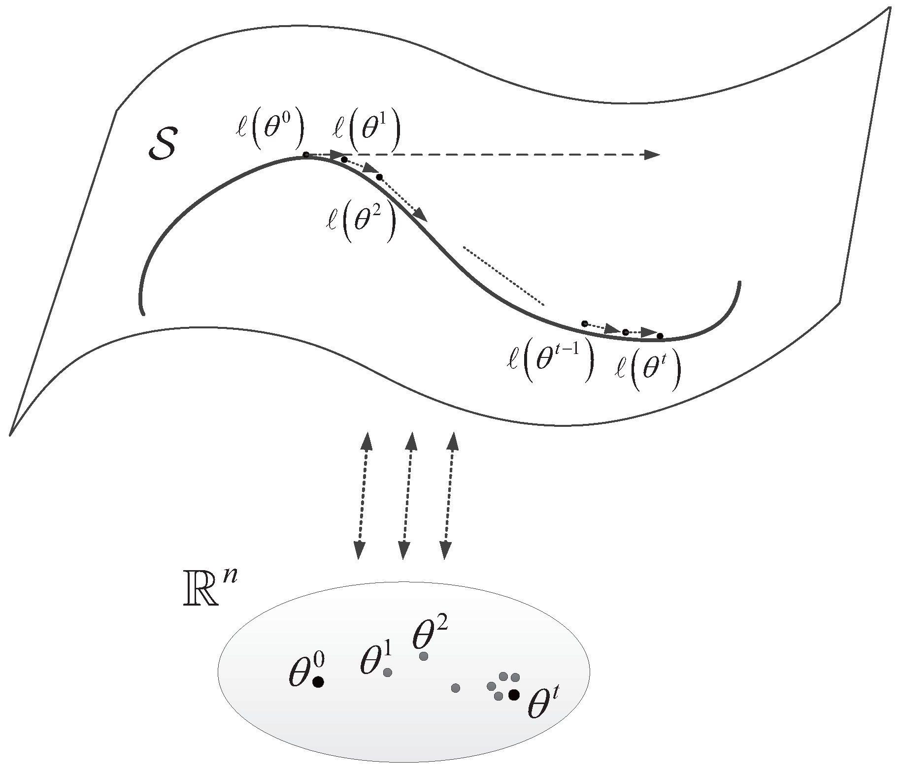
The geometric interpretation of this method is that the process path has moved from point P to point Q in the manifold $\mathcal{S}$ along the steepest direction, while the parameter has moved from ${\theta }^p$ to ${\theta }^q$ in parameter space. As the process path has been moving in the manifold $\mathcal{S}$, the parameter has been estimated recursively. The recursive formation as follow

$$\begin{array}{c}\hfill {\theta }^{t+1}={\theta }^t+\eta {\mathbf{G}}^{-1}\left({\theta }^t\right)\nabla \ell \left({\theta }^t\right)\end{array}$$

(22)

where t denotes the times of iterative procedure in which correspond with the iterated points in the statistical manifold. This iteration procedure has been illustrated in Figure 1.

For the recursive process, we can use KLD, which is often used to show the discrepancy between two probability distributions, as the stopping criterion. It is defended by

$$\begin{array}{c}\hfill D[{\theta }^p:{\theta }^q]=\int p\left(y;{\theta }^p\right)log\frac{p\left(y;{\theta }^p\right)}{p\left(y;{\theta }^q\right)}dy\end{array}$$

(23)

where $p\left(y;{\theta }^p\right)$ and $p\left(y;{\theta }^p\right)$ as the specification with respect to two parameters ${\theta }^p$ and ${\theta }^q$, respectively. When the two probability distributions are infinitesimally close, corresponding with ${\theta }^q={\theta }^p+d\theta$, the KLD between two nearby distributions can be expanded as

$$\begin{array}{c}\hfill D[{\theta }^p:{\theta }^p+d\theta ]=\frac{1}{2}d{\theta }^{\mathrm{T}}\mathbf{G}\left(\theta \right)d\theta \end{array}$$

(24)

Motivated by the relationship between the statistical manifold and the parameter space, the estimation of state conditional on the measurement in state parameter space can be converted to the iteration procedure on the manifold in which constructed by the posterior PDF. This method provides a new alternative for the measurement update in nonlinear filtering based on the Bayesian framework.

3. Filtering Based on Information Geometry

In this section, we present the ideas of measurement update based on the natural gradient descent. In Bayesian framework, the predicted state acts as the prior information with respect to the state to deduce the posterior distribution under the condition of measurements. Then the natural gradient descent method has been used to estimation the final state recursively. Here, we consider the usual scenario which discrete-time state space as follow

$$\begin{array}{cc}\hfill x_k& =f\left(x_{k-1}\right)+w_k\hfill \end{array}$$

(25)

$$\begin{array}{cc}\hfill y_k& =h\left(x_k\right)+v_k\hfill \end{array}$$

(26)

where $x_k\in {\mathbb{R}}^n$ and $y_k\in {\mathbb{R}}^m$ denote the system discrete-time state and measurement at the instant k respectively, f and h denote the state transition and measurement functions. $w_k$ and $v_k$ are the noise correspondence with state and measurement respectively. Generally the additive white Gaussian noise (AWGN) has been studied for simplicity.

In Bayesian filtering, the time propagation can be processed according to the state transition function, and the prediction of state can be achieved in this step. Based on the Bayesian principle, the prediction of state is considered as the prior information about the state.

$$\begin{array}{cc}\hfill p\left({\widehat{x}}_k^{-}\right)& =p\left(x_k|{\mathbf{y}}_{k-1}\right)\hfill \\ & =\int p\left(x_k|x_{k-1}\right)p\left(x_{k-1}|{\mathbf{y}}_{k-1}\right)d{x}_{k-1}\hfill \\ & =\int p\left(x_k|x_{k-1}\right)p\left(x_{k-1}|y_{k-1}\right)d{x}_{k-1}\hfill \end{array}$$

(27)

where ${\mathbf{y}}_{k-1}=\{y_{k-1},y_{k-2},\dots ,y_1\}$. The relationship $p\left(x_{k-1}|{\mathbf{y}}_{k-1}\right)=p\left(x_{k-1}|y_{k-1}\right)$ means that the current state only depends on current measurement and is conditionally independent from all past measurements. The PDF $p\left(x_k|x_{k-1}\right)$ and $p\left(x_{k-1}|y_{k-1}\right)$ denote the state transition PDF and posterior PDF of state for last time, respectively. To aim at obtaining the posterior PDF of current time under the condition of current measurement, we can use the Bayesian principle for deducing. The procedure of the measurement update in the form of Bayesian filtering as

$$\begin{array}{cc}\hfill p\left({\widehat{x}}_k^{+}\right)& =p\left(x_k|{\mathbf{y}}_k\right)\hfill \\ & =\frac{p\left(x_k,y_k|{\mathbf{y}}_{k-1}\right)p\left({\mathbf{y}}_{k-1}\right)}{p\left(y_k|{\mathbf{y}}_{k-1}\right)p\left({\mathbf{y}}_{k-1}\right)}\hfill \\ & =\frac{p\left(y_k|x_k,{\mathbf{y}}_{k-1}\right)p\left(x_k|{\mathbf{y}}_{k-1}\right)}{\int p\left(y_k|x_k,{\mathbf{y}}_{k-1}\right)p\left(x_k|{\mathbf{y}}_{k-1}\right)d{x}_k}\hfill \\ & =\frac{p\left(y_k|x_k\right)p\left(x_k|y_{k-1}\right)}{\int p\left(y_k|x_k\right)p\left(x_k|y_{k-1}\right)d{x}_k}\hfill \end{array}$$

(28)

since the likelihood $p\left(y_k|x_k,{\mathbf{y}}_{k-1}\right)=p\left(y_k|x_k\right)$, i.e., the measurement $y_k$ is conditionally independent of all past measurements. The denominator of the posterior PDF is the normalizing constant independent of the state. Thus the posterior PDF can be rewrite as

$$\begin{array}{cc}\hfill p\left({\widehat{x}}_k^{+}\right)& =p\left(x_k|y_k\right)\hfill \\ & \propto p\left(y_k|x_k\right)p\left(x_k|y_{k-1}\right)\hfill \\ & =p\left(y_k|x_k\right)p\left({\widehat{x}}_k^{-}\right)\hfill \end{array}$$

(29)

where ∝ means “is proportional to”. $p\left({\widehat{x}}_k^{-}\right)$ and $p\left(y_k|x_k\right)$ are the prior and the likelihood respectively. In this paper, we assume that they are all Gaussian distribution for simplicity, which the Gaussian approximation has been used for non-Gaussian distribution and beyond our paper. Based on the procedure of state propagation, the prior distribution can be described as

$$\begin{array}{c}\hfill p\left({\widehat{x}}_k^{-}\right)=\frac{exp\left[-\frac{1}{2}{\left(x_k-{\widehat{x}}_k^{-}\right)}^{\mathrm{T}}{\mathbf{P}}^{-1}\left(x_k-{\widehat{x}}_k^{-}\right)\right]}{\sqrt{{\left(2\pi \right)}^n\left|\mathbf{P}\right|}}\end{array}$$

(30)

Usually, the likelihood with respect to the measurement is chosen as

$$\begin{array}{c}\hfill p\left(y_k|x_k\right)=\frac{exp\left[-\frac{1}{2}{\left(y_k-h\left(x_k\right)\right)}^{\mathrm{T}}{\mathbf{R}}^{-1}\left(y_k-h\left(x_k\right)\right)\right]}{\sqrt{{\left(2\pi \right)}^m\left|\mathbf{R}\right|}}\end{array}$$

(31)

where $|·|$ is the determinant, n and m are the number of dimension of state and measurement, respectively.

In the stage of measurement update, the goal is to obtain the optimal estimation of state under the conditions of the corresponding measurement and the prior information of state. From the Bayesian perspective, it is the maximum a posterior PDF of the prior and the likelihood. This MAP method has been used in the estimation for statistical signal processing extensively. With the optimization view, the solution that maximizes $p\left({\widehat{x}}_k^{+}\right)$ is equivalent to minimizing its negative log likelihood function. The negative log operation of posterior distribution is

$$\begin{array}{cc}\hfill L\left(x_k\right)& =-logp({\widehat{x}}_k^{+})\hfill \\ & =\frac{1}{2}{(x_k-{\widehat{x}}_k^{-})}^{\mathrm{T}}{\mathbf{P}}^{-1}(x_k-{\widehat{x}}_k^{-})+\frac{1}{2}(y_k-h(x_k){)}^{\mathrm{T}}{\mathbf{R}}^{-1}(y_k-h(x_k))+C\hfill \end{array}$$

(32)

where C is a constant which not effect the estimation of state $x_k$. Defining the negative log likelihood function

$$\begin{array}{cc}\hfill \ell (x_k)& =\frac{1}{2}{(x_k-{\widehat{x}}_k^{-})}^{\mathrm{T}}{\mathbf{P}}^{-1}(x_k-{\widehat{x}}_k^{-})+\frac{1}{2}{(h(x_k)-y_k)}^{\mathrm{T}}{\mathbf{R}}^{-1}(h(x_k)-y_k)\hfill \end{array}$$

(33)

thus the object function can be convert into

$$\begin{array}{c}\hfill \underset{x_k}{max}p({\widehat{x}}_k^{+})=\underset{x_k}{min}\ell (x_k)\end{array}$$

(34)

Based on the posterior PDF, the statistical manifold $\mathcal{S}$ can be defined as

$$\begin{array}{c}\hfill \mathcal{S}=\{p(x_k|y_k)\}\end{array}$$

(35)

Meanwhile, the negative log function as the mapping from $\mathcal{S}$ to $\mathbb{R}$, i.e., $\ell :\mathit{S}\to \mathbb{R}$ has constructed the coordinate system.

Let ${\ell }_1$ and ${\ell }_2$ stand for the first and second part of the Equation (33), $e_y=h\left(x_k\right)-y_k$ and $e_x=x_k-{\widehat{x}}_k^{-}$ for the error of measurement and the state estimation respectively. Computing the first derivative of ${\ell }_1$ and ${\ell }_2$ about the $x_k$ and $x_k^{\mathrm{T}}$ respectively

$$\begin{array}{cc}\hfill \frac{\partial {\ell }_1}{\partial x_k}& ={\left(\partial h\right)}^{\mathrm{T}}{\mathbf{R}}^{-1}{e}_y\hfill \end{array}$$

(36)

$$\begin{array}{cc}\hfill \frac{\partial {\ell }_1}{\partial x_k^{\mathrm{T}}}& =e_y^{\mathrm{T}}{\mathbf{R}}^{-1}\left(\partial h\right)\hfill \end{array}$$

(37)

$$\begin{array}{cc}\hfill \frac{\partial {\ell }_2}{\partial x_k}& ={\mathbf{P}}^{-1}{e}_x\hfill \end{array}$$

(38)

$$\begin{array}{cc}\hfill \frac{\partial {\ell }_2}{\partial x_k^{\mathrm{T}}}& =e_x^{\mathrm{T}}{\mathbf{P}}^{-1}\hfill \end{array}$$

(39)

where $\partial h=\frac{\partial h\left(x_k\right)}{\partial x_k}\in {\mathbb{R}}^m\times {\mathbb{R}}^n$ denotes the Jacobian of $h\left(x_k\right)$ about $x_k$. The covariance matrix ${\mathbf{R}}^{-1}$ and ${\mathbf{P}}^{-1}$ are symmetry. Thus the gradient of the negative log likelihood is

$$\begin{array}{c}\hfill \nabla \ell \left(x_k\right)={\left(\partial h\right)}^{\mathrm{T}}{\mathbf{R}}^{-1}{e}_y+{\mathbf{P}}^{-1}{e}_x\end{array}$$

(40)

Then the Fisher metric $\mathbf{G}$ of manifold $\mathcal{S}$ can be obtained

$$\begin{array}{cc}\hfill \mathbf{G}\left(x_k\right)& =\mathbf{E}\left[\frac{\partial \ell }{\partial x_k}{\left(\frac{\partial \ell }{\partial x_k}\right)}^{\mathrm{T}}\right]=-\mathbf{E}\left[\frac{{\partial }^2\ell }{\partial x_k\partial x_k^{\mathrm{T}}}\right]\hfill \\ & =-\mathbf{E}\left[\frac{\partial }{\partial x_k}\left({e_y}^{\mathrm{T}}{\mathbf{R}}^{-1}\left(\partial h\right)+e_x^{\mathrm{T}}{\mathbf{P}}^{-1}\right)\right]\hfill \\ & =-\mathbf{E}\left[e_y^{\mathrm{T}}{\mathbf{R}}^{-1}\left({\partial }^{2}h\right)+{\left(\partial h\right)}^{\mathrm{T}}{\mathbf{R}}^{-1}\left(\partial h\right)+{\mathbf{P}}^{-1}\right]\hfill \\ & =-{\left(\partial h\right)}^{\mathrm{T}}{\mathbf{R}}^{-1}\left(\partial h\right)-{\mathbf{P}}^{-1}\hfill \end{array}$$

(41)

where ${\partial }^{2}h=\frac{{\partial }^{2}h\left(x_k\right)}{\partial x_k\partial x_k^{\mathrm{T}}}\in {\mathbb{R}}^m\times {\mathbb{R}}^n\times {\mathbb{R}}^n$ and $\mathrm{E}$ denotes the expectation with respect to the measurement $y_k$. In the above deducing procedure, the follow principle has been used

$$\begin{array}{c}\hfill D_x\left(\mathbf{f}{\left(x\right)}^{\mathrm{T}}\mathbf{Ag}\left(x\right)\right)=\mathbf{g}{\left(x\right)}^{\mathrm{T}}{\mathbf{A}}^{\mathrm{T}}{D}_x\mathbf{f}\left(x\right)+\mathbf{f}{\left(x\right)}^{\mathrm{T}}\mathbf{A}{D}_x\mathbf{g}\left(x\right)\end{array}$$

(42)

With the computed gradient and Fisher metric, the natural gradient of manifold is

$$\begin{array}{cc}\hfill \mathbf{G}{\left(x_k\right)}^{-1}\nabla \ell \left(x_k\right)& =-{\left({\left(\partial h\right)}^{\mathrm{T}}{\mathbf{R}}^{-1}\left(\partial h\right)+{\mathbf{P}}^{-1}\right)}^{-1}\left({\left(\partial h\right)}^{\mathrm{T}}{\mathbf{R}}^{-1}{e}_y+{\mathbf{P}}^{-1}{e}_x\right)\hfill \end{array}$$

(43)

Meanwhile, considering the denominator of Equation (20), it can be computed as

$$\begin{array}{cc}& \nabla \ell {\left(x_k\right)}^{\mathrm{T}}\mathbf{G}{\left(x_k\right)}^{-1}\nabla \ell \left(x_k\right)\hfill \\ & =tr\left[\mathbf{G}{\left(x_k\right)}^{-1}\nabla \ell \left(x_k\right)\nabla \ell {\left(x_k\right)}^{\mathrm{T}}\right]\hfill \\ & =tr\left[{(\partial h^{\mathrm{T}}{\mathbf{R}}^{-1}\partial h+{\mathbf{P}}^{-1})}^{-1}(\partial h^{\mathrm{T}}{\mathbf{R}}^{-1}{e}_y+{\mathbf{P}}^{-1}{e}_x){(\partial h^{\mathrm{T}}{\mathbf{R}}^{-1}{e}_y+{\mathbf{P}}^{-1}{e}_x)}^{\mathrm{T}}\right]\hfill \\ & =tr\left[{(\partial h^{\mathrm{T}}{\mathbf{R}}^{-1}\partial h+{\mathbf{P}}^{-1})}^{-1}(\partial h^{\mathrm{T}}{\mathbf{R}}^{-1}{e}_y{e}_y^{\mathrm{T}}{\mathbf{R}}^{-1}\partial h+\partial h^{\mathrm{T}}{\mathbf{R}}^{-1}{e}_y{e}_x^{\mathrm{T}}{\mathbf{P}}^{-1}+{\mathbf{P}}^{-1}{e}_x{e}_y^{\mathrm{T}}{\mathbf{R}}^{-1}\partial h+{\mathbf{P}}^{-1}{e}_x{e}_x^{\mathrm{T}}{\mathbf{P}}^{-1})\right]\hfill \end{array}$$

(44)

For simplicity, we use the expectation value to substitute the value which computed in each iterative procedure. Thus

$$\begin{array}{cc}& \mathbf{E}\left[\mathbf{G}{\left(x_k\right)}^{-1}\nabla \ell \left(x_k\right)\nabla \ell {\left(x_k\right)}^{\mathrm{T}}\right]\hfill \\ & ={\left(\partial h^{\mathrm{T}}{\mathbf{R}}^{-1}\partial h+{\mathbf{P}}^{-1}\right)}^{-1}\left(\partial h^{\mathrm{T}}{\mathbf{R}}^{-1}\mathbf{R}{\mathbf{R}}^{-1}\partial h+{\mathbf{P}}^{-1}\mathbf{P}{\mathbf{P}}^{-1}\right)\hfill \\ & ={\left(\partial h^{\mathrm{T}}{\mathbf{R}}^{-1}\partial h+{\mathbf{P}}^{-1}\right)}^{-1}\left(\partial h^{\mathrm{T}}{\mathbf{R}}^{-1}\partial h+{\mathbf{P}}^{-1}\right)\hfill \\ & =\mathbf{I}\hfill \end{array}$$

(45)

where $e_y$ and $e_x$ are independent, and $\mathbf{I}$ is the n-dimension square matrix which correspondence to the n-dimension state. Based on the natural gradient descent, we can construct the recursive procedure to get the optimal estimation in the measurement update step

$$\begin{array}{cc}\hfill x_k^t& =x_k^{t-1}+\frac{\epsilon }{\sqrt{\nabla \ell {\left(x_k^{t-1}\right)}^{\mathrm{T}}{\mathbf{G}}^{-1}\nabla \ell \left(x_k^{t-1}\right)}}{\mathbf{G}}^{-1}\left(x_k^{t-1}\right)\nabla \ell \left(x_k^{t-1}\right)\hfill \\ & \approx x_k^{t-1}+\frac{\epsilon }{\sqrt{tr\left(\mathbf{I}\right)}}{\mathbf{G}}^{-1}\left(x_k^{t-1}\right)\nabla \ell \left(x_k^{t-1}\right)\hfill \\ & \approx x_k^{t-1}+\frac{\epsilon }{\sqrt{n}}{\mathbf{G}}^{-1}\left(x_k^{t-1}\right)\nabla \ell \left(x_k^{t-1}\right)\hfill \end{array}$$

(46)

where n is the dimension of the state. Replacing the parameter as $\eta =\frac{\epsilon }{\sqrt{n}}$, the natural gradient descent method becomes the simplification form suggested by Amari. Given the above, the iterative procedure for estimating the state can be constructed

$$\begin{array}{cc}\hfill x_k^t& =x_k^{t-1}+\eta {\mathbf{G}}^{-1}\left(x_k^{t-1}\right)\nabla \ell \left(x_k^{t-1}\right)\hfill \\ & =x_k^{t-1}+\eta {\left(\partial h^{\mathrm{T}}{\mathbf{R}}^{-1}\partial h+{\mathbf{P}}_{t-1}^{-1}\right)}^{-1}{\left.\left(\partial h^{\mathrm{T}}{\mathbf{R}}^{-1}\left(y_k-h\left(x_k\right)\right)+{\mathbf{P}}_{t-1}^{-1}(x_k^{t-1}-x_k)\right)\right|}_{x_k=x_k^{t-1}}\hfill \\ & =x_k^{t-1}+\eta {\left(\partial h_{t-1}^{\mathrm{T}}{\mathbf{R}}^{-1}\partial h_{t-1}+{\mathbf{P}}_{t-1}^{-1}\right)}^{-1}\left(\partial h_{t-1}^{\mathrm{T}}{\mathbf{R}}^{-1}\right)\left(y_k-h\left(x_k^{t-1}\right)\right)\hfill \end{array}$$

(47)

where $\partial h_{t-1}=\frac{\partial h\left(x_k\right)}{\partial x_k}{\mid }_{x_k=x_k^{t-1}}$, and ${\mathbf{P}}_{t-1}$ is the covariance matrix after the $t-1$ iterative procedure.

For the iterative procedure, a stopping criterion should be set for final estimation. In the statistical manifold, the KLD is a better criterion for measurement the distance between two PDF. Because of the estimated state corresponding with the posterior PDF, the convergence in statistical manifold also means the better estimation in parameter space. Besides, Morelande [15] has shown that the lower KLD value to select the optimum parameter for the approximation posterior PDF has better performance. Thus, we choose the KLD as the stopping criterion in the iteration procedure of measurement update following the statistical manifold.

$$\begin{array}{c}\hfill D[x_k^{t-1}:x_k^k]=\frac{1}{2}{(x_k^k-x_k^{t-1})}^{\mathrm{T}}\mathbf{G}\left(x_k^{t-1}\right)(x_k^k-x_k^{t-1})\le \delta \end{array}$$

(48)

Also, we can choose a stopping criterion as the follow form from the view of parameter space in which has been used in the IEKF or other iterated estimation problems

$$\begin{array}{c}\hfill \parallel {\widehat{x}}_k^t-{\widehat{x}}_k^{t-1}{\parallel }_2^2\le \gamma \end{array}$$

(49)

Based on this measurement update method, we can construct nonlinear filtering by combining the existing method for state propagation. Here, we use the Ensemble Kalman filter (EnKF) for state propagation, which uses the Monte Carlo technique for integral operation in the Bayesian filtering. For the last procedure ensemble has $N_s$ elements as

$$\begin{array}{c}\hfill S_{k-1|k-1}=\{{\widehat{x}}_{k-1|k-1}^i,i=1,\cdots ,N_s\}\end{array}$$

(50)

We can get the prediction ensemble as

$$\begin{array}{c}\hfill S_{k|k-1}=\{{\widehat{x}}_{k|k-1}^i=f({\widehat{x}}_{k-1|k-1}^i)+w_k^i,i=1,\cdots ,N_s\}\end{array}$$

(51)

where $w_k^i$ is generated according the state process noise. Then, the mean and the covariance matrix can be computed

$$\begin{array}{cc}\hfill {\overline{x}}_{k|k-1}& =\frac{1}{N_s}\sum _{i=1}^{N_s}{\widehat{x}}_{k|k-1}^i\hfill \end{array}$$

(52)

$$\begin{array}{cc}\hfill {\mathbf{P}}_{k|k-1}& =\frac{1}{N_s-1}\sum _{i=1}^{N_s}({\widehat{x}}_{k|k-1}^i-{\overline{x}}_{k|k-1}){({\widehat{x}}_{k|k-1}^i-{\overline{x}}_{k|k-1})}^{\mathrm{T}}\hfill \end{array}$$

(53)

In the Bayesian framework, these prediction means and covariance will be incorporated in the procedure as prior information of state to propel the measurement update by the natural gradient method. With the stopping criterion of iterative procedure, we can get the final estimation of state. Meanwhile, the iterative estimation will converge to its final value because of the convergence of the natural gradient descent, and the iterative procedure can process some iterative estimation value of state. Here, we consider these values as the ensemble of measurement update for next period of nonlinear filter in the EnKF.

$$\begin{array}{c}\hfill S_{k|k}=\{{\widehat{x}}_{k|k}^i,i=1,\cdots ,N_s\}\end{array}$$

(54)

Thus, the complete nonlinear filter method has proposed based on state propagation by EnKF and measurement update by natural gradient descent method, and has been shown in Algorithm 1.

Algorithm 1 Natural Gradient Descent Method for Measurement Update in EnKF

Input: Measurement $\mathbf{y}=\{y_1,y_2,...,y_T\}$, ensemble $N_s$, parameter $\eta \in (0,1]$.

Initialize: $x_0$, ${\mathbf{P}}_0$, ${\widehat{x}}_0^i=x_0+\sqrt{{\mathbf{P}}_0}\mathcal{N}(0,1)$, ensemble $S_{0|0}=\{{\widehat{x}}_0^i,i=1,...,N_s\}$.

For $k=1:T$

% compute prediction ensemble

$S_{k|k-1}=\{{\widehat{x}}_{k|k-1}^i=f({\widehat{x}}_{k-1|k-1}^i)+w_k^i,i=1,...,N_s\}$;

% compute mean and covariance of prediction ensemble

${\overline{x}}_{k|k-1}=\frac{1}{N_s}{\sum }_{i=1}^{N_s}{\widehat{x}}_{k|k-1}^i$;

${\mathbf{P}}_{k|k-1}=\frac{1}{N_s-1}{\sum }_{i=1}^{N_s}({\widehat{x}}_{k|k-1}^i-{\overline{x}}_{k|k-1}){({\widehat{x}}_{k|k-1}^i-{\overline{x}}_{k|k-1})}^{\mathrm{T}}$;

% natural gradient descent for measurement update

$x_{k|k}^0={\overline{x}}_{k|k-1}$, ${\mathbf{P}}_{k|k}^0={\mathbf{P}}_{k|k-1}$ , $t=1$;

For $t=1:N_s$

${\mathbf{H}}_{t-1}={\left.\frac{\partial h(x_k)}{\partial x_k}\right|}_{x_k=x_{k|k}^{t-1}}$ ;

$\mathbf{G}={\mathbf{H}}_{t-1}^{\mathrm{T}}{\mathbf{R}}^{-1}{\mathbf{H}}_{t-1}+{\left({\mathbf{P}}_{k|k}^{t-1}\right)}^{-1}$;

$\nabla \ell =\left({\mathbf{H}}_{t-1}^{\mathrm{T}}{\mathbf{R}}^{-1}\right)\left(y_k-h(x_k^{t-1})\right)$;

$x_{k|k}^t=x_{k|k}^{t-1}+\eta {\mathbf{G}}^{-1}\nabla \ell$;

${\mathbf{P}}_{k|k}^t=\frac{1}{N_s-1}{\sum }_{i=1}^{N_s}({\widehat{x}}_{k|k-1}^i-x_{k|k}^t){({\widehat{x}}_{k|k-1}^i-x_{k|k}^t)}^{\mathrm{T}}$;

$\mathbf{D}[x_k^{t-1}:x_k^t]=\frac{1}{2}{(x_{k|k}^t-x_{k|k}^{t-1})}^{\mathrm{T}}\mathbf{G}(x_{k|k}^t-x_{k|k}^{t-1})$;

End for

% Select final estimation

For $t=1:N_s$

If $\mathbf{D}[x_k^{t-1}:x_k^t]\le \delta$ and $\parallel {\widehat{x}}_{k|k}^t-{\widehat{x}}_{k|k}^{t-1}{\parallel }_2^2\le \gamma$

${\widehat{x}}_{k|k}=x_{k|k}^t$;

${\mathbf{P}}_{k|k}={\mathbf{P}}_{k|k}^t$;

End if

End for

$S_{k|k}=\{x_{k|k}^t,i=1,...,N_s\}$;

End for

Output: State $\mathbf{x}=\{{\widehat{x}}_{k|k},k=1,...,T\}$

4. Comparing with the Existing Methods

As the natural gradient descent method for measurement update, we can get some conclusions comparing with the existing methods. When we choose the parameter as $\eta =1$ with a single iteration, the iterative procedure (47) will be simplified as

$$\begin{array}{cc}\hfill x_k=x_{k-1}+& {\left(\partial h_{k-1}^{\mathrm{T}}{\mathbf{R}}^{-1}\partial h_{k-1}+{\mathbf{P}}^{-1}\right)}^{-1}\left(\partial h_{k-1}^{\mathrm{T}}{\mathbf{R}}^{-1}\right)\left(y_k-h\left(x_{k-1}\right)\right)\hfill \end{array}$$

(55)

Thus, the update has deduced to the traditional Kalman filter and the EKF. When the measurement function is linear, i.e., $y_k=h\left(x_k\right)=\mathbf{H}{x}_k$, the Jacobian of $h\left(x_k\right)$ can be obtained easily as $\frac{\partial h\left(x_k\right)}{\partial x_k}=\mathbf{H}$, $\frac{\partial h\left(x_k\right)}{\partial x_k^{\mathrm{T}}}={\mathbf{H}}^{\mathrm{T}}$. As for the nonlinear measurement function, the first-order Taylor expansion has been used as the same as the linear case. The procedure becomes

$$\begin{array}{cc}\hfill x_k& =x_{k-1}+{\left({\mathbf{H}}^{\mathrm{T}}{\mathbf{R}}^{-1}\mathbf{H}+{\mathbf{P}}^{-1}\right)}^{-1}\left({\mathbf{H}}^{\mathrm{T}}{\mathbf{R}}^{-1}\left(y_k-h\left(x_{k-1}\right)\right)\right)\hfill \\ & =x_{k-1}+\left(\mathbf{P}{\mathbf{H}}^{\mathrm{T}}\right){\left(\mathbf{H}\mathbf{P}{\mathbf{H}}^{\mathrm{T}}+\mathbf{R}\right)}^{-1}\left(y_k-h\left(x_{k-1}\right)\right)\hfill \end{array}$$

(56)

where the matrix inversion lemma

$$\begin{array}{c}\hfill {({\mathbf{H}}^{\mathrm{T}}{\mathbf{R}}^{-1}\mathbf{H}+{\mathbf{P}}^{-1})}^{-1}{\mathbf{H}}^{\mathrm{T}}{\mathbf{R}}^{-1}=\mathbf{P}{\mathbf{H}}^{\mathrm{T}}{({\mathbf{HPH}}^{\mathrm{T}}+\mathbf{R})}^{-1}\end{array}$$

(57)

has been used in the simplification. In comparison, this is the same as the measurement update in traditional Kalman filter and EKF.

Besides, there are two iteration methods existing before. The one is IEKF [12,32], which also has been derived based on the MAP method. Its update step has the form as

$$\begin{array}{cc}\hfill x_k^t={\widehat{x}}_k^{-}+& \left(\mathbf{P}{\mathbf{H}}_{t-1}^{\mathrm{T}}\right){\left({\mathbf{H}}_{t-1}\mathbf{P}{\mathbf{H}}_{t-1}^{\mathrm{T}}+\mathbf{R}\right)}^{-1}\left(y_k-h(x_k^{t-1})-{\mathbf{H}}_{t-1}({\widehat{x}}_k^{-}-x_k^{t-1})\right)\hfill \end{array}$$

(58)

where ${\mathbf{H}}_{t-1}={\left.\frac{\partial h\left(x_k\right)}{\partial x_k}\right|}_{x_k=x_k^{t-1}}$.

Comparing with IEKF and our proposed method, there are some differences. Firstly, the initial estimation value in each iteration is the same as the prior estimation in the IEKF, while our proposed method bases on the last iterated estimation. Secondly, the parameter η of the natural gradient descent controls the update step of state, but the IEKF has no parameters to control the update step. Thirdly, the innovations are used in the natural gradient descent method, while the IEKF adds the prediction error of current estimation state and the prior estimation state. Further from the formulation of the IEKF update, the first step of IEKF is identified to the EKF, and later steps are from the direction of overestimation convergence to the true state.

Another iteration method is RUF [9], which derived based on the LMMSE method. It defines the cross-covariance between the measurement noise and the estimation error for each steps. Then the LMMSE method has been used to deduce the update step. Also, it has considered the fraction of update, which selected as the reciprocal of the number of iteration steps. In comparison with our proposed method, the RUF uses the manual setting number of iteration steps, which also influences the update step, and has no criterion for evaluation the estimation performance. In some case, the other criterions may provide guarantee for convergence and performance in the procedure. Moreover the detailed differences among these methods will be discussed in the numerical examples in the next section.

5. Numerical Examples

In this section, we present three numerical examples to demonstrate the advantages of our proposed method and illustrate the differences between the proposed method and the existing method. The first scalar example provides a good geometrical interpretation in the convergence speed and the iteration procedure. The second example, which has been used as the common test platform for nonlinear filtering in scalar, is provided to validate the performance. The third example is a multidimensional filtering problem in which has tracked a vehicle entering atmosphere.

5.1. Iteration and Convergence for Measurement Update

Consider a sample scalar nonlinear measurement as

$$\begin{array}{c}\hfill y=x^5+v\end{array}$$

(59)

where x denotes the state, and y denotes the measurement with noise $v\sim \mathcal{N}(0,0.1^2)$. Only for the measurement update step, we assume the mean and variance of prediction state, which as prior information in the Bayesian framework, are ${\widehat{x}}^{-}=2.5$ and $\mathbf{P}=0.5^2$, and the true state value is set at $x=4$. With noisy measuring, the measurement $y=1024.4$. We compare our proposed method with EKF, IEKF, and RUF. The results are shown in the Figure 2. The EKF only has one step in the procedure for estimation the posterior, while the other methods have more than one steps. For the IEKF method, the results illustrate that the first step of IEKF is the same as the EKF, which also can be deduced from the expression of two methods. However, the more iteration steps in the IEKF make the estimation converge to the true posterior state. In detail, the second and more iteration steps in the IEKF have the same beginning state for estimation, but the ending state after estimation is more close to true state. Completing the procedure, the more steps in the IEKF, the more accurate estimation than the EKF. Considering the RUF, the error of estimation is incorporated in the to refine the estimation. After some iterated steps, the error would be approximately reduced to zero. Thus the final estimation is convergence to the true state. For our proposed method, the parameter η controls the convergence behaviours to true state. When the parameter $\eta =0.8$, the first step for estimation is bigger than the true state as same as the EKF, then the later iteration steps convergence to true state in the contrary direction of RUF. As the parameter $\eta =0.2$, the convergence path of iteration steps is the same direction of RUF, but has the fast convergence speed. Moreover, we consider the convergence of the natural gradient descent method. We use the random technique to generate the initial state and parameter $\eta =0.5$. The results are show in Figure 3 after running 100 Monte Carlo. It has showed that the iteration steps, which the natural gradient descent convergence to the true state, always need less 30 times.

5.2. Univariate Nonstationary Growth Model (UNGM)

This model has been used extensively to validate the performance of nonlinear filtering because of its high nonlinearity. The model can be formulated as [33]

$$\begin{array}{cc}\hfill x_k& =\frac{x_{k-1}}{2}+\frac{25x_{k-1}}{1+x_{k-1}^2}+8cos(1.2k)+u_k\hfill \end{array}$$

(60)

$$\begin{array}{cc}\hfill y_k& =\frac{x_k^3}{20}+v_k\hfill \end{array}$$

(61)

where $u_k$ and $v_k$ denote the additive white Gaussian noise corresponding with state and measurement, as $u_k\sim \mathcal{N}(0,Q)$ and $v_k\sim \mathcal{N}(0,R)$. In this experiment, we set the variance as $Q=10$ and $R=1$, respectively. We assume the initiate state as $p\left(x_0\right)=\mathcal{N}(x_0;0,1)$ before the filtering procedure. The true state that we used in the simulations with 100 time steps has a severe fluctuation, which has showed in the Figure 4. The state varies frequently, and the first order Taylor series expanded can not depict fitting in the procedure. Thus, the EKF has the bad performance in the experiment. In addition, the state will make the nonlinear measurement more difficult.

As a performance metric, we use Root Mean Square Error (RMSE) in the example. Let ${\widehat{x}}_k^i$ and $x_k^i$ denote the estimated state and true state at time k, respectively. Then the RMSE is defined as

$$\begin{array}{c}\hfill {\mathrm{RMSE}}_k=\sqrt{\frac{1}{M}{\displaystyle \sum _{i=1}^M}{\left({\widehat{x}}_k^i-x_k^i\right)}^2}\end{array}$$

where M is the total number of Monte Carlo runs.

In our experiment, the RMSE is obtained by using 100 Monte Carlo runs, averaging over different realizations of the measurements and the true states. The comparison is achieved between our proposed method, which called natural gradient descent Kalman filter (NgdKF) here, and the four existing methods, i.e., EnKF, IEKF, EKF, and RUF. In the EnKF and our proposed method, the number of ensemble used each time is 200, and the initial ensemble generated randomly with $p\left(x_0\right)$. During the procedure of IEKF, the stopping criterion is $\parallel {\widehat{x}}_{k|k}^t-{\widehat{x}}_{k|k}^{t-1}{\parallel }_2^2\le {10}^{-4}$, while $\parallel {\widehat{x}}_{k|k}^t-{\widehat{x}}_{k|k}^{t-1}{\parallel }_2^2\le {10}^{-4}$ and $\mathbf{D}[x_k^{t-1}:x_k^t]\le {10}^{-5}$ in our proposed method. The number of iteration steps in the RUF is set as 200. The parameter $\eta =0.5$ is selected in our proposed method for the iterated step by natural gradient descent method. The comparison results measured by the RMSE are showed in the Figure 5. As we can see that our proposed method performs much better than EKF, EnKF, RUF, and IEKF. As aforementioned in the Figure 4, the EKF becomes poor because of first order Taylor series expanded is not fit the measurement function. In comparing the iteration methods, i.e., IEKF, RUF and NgdKF, with no iteration method, i.e., EKF and EnKF, the front class methods have the better performance than the later. This conclusion also has been mentioned by Lefebvre [14]. However, the later is computed faster than the front. In fact, from the update formulation of each method, the iteration methods have more than one steps, while the no iteration only has one step. In the nonlinear filter, we have to take more times or steps to improve the filtered precision. Based on the comparison results, our proposed method has the better performance.

5.3. Tracking of Vehicle Entering Atmosphere

In the previous example, we have shown the performance in scalar filtering problem. In this example, we will study a multidimensional dynamic system. We analyze target tracking problem of a vehicle entering atmosphere at high altitude with a high speed [34]. It has the continuous state, which constructed by position ($x_1$ and $x_2$), velocity ($x_3$ and $x_4$) and drag coefficient ($x_5$), and the discrete measurement constructed by range ($r_k$) and bearing ($b_k$). This experiment is a better platform to measure the filtering algorithms. Firstly, the number of dimension between the state and the measurement is difference. Secondly, the noise is partial in the state propagation. Thirdly, the measurement function is nonlinear. Fourthly, the drag coefficient is a constant but affected by the noise, which can give a good criterion for measuring the filtering performance.

With the vector description of the continuous state as $X\left(t\right)={\left[x_1\left(t\right),x_2\left(t\right),x_3\left(t\right),x_4\left(t\right),x_5\left(t\right)\right]}^{\mathrm{T}}\in {\mathbb{R}}^5$, and the discrete-time measurement as $Y\left(k\right)={\left[r\left(k\right),b\left(k\right)\right]}^{\mathrm{T}}\in {\mathbb{R}}^2$, the state equation of dynamic is characterized as

$$\begin{array}{c}\hfill \dot{X}\left(t\right)=F\left(t\right)X\left(t\right)+W\left(t\right)\end{array}$$

(62)

where $\dot{X}\left(t\right)={\left[{\dot{x}}_1\left(t\right),{\dot{x}}_2\left(t\right),{\dot{x}}_3\left(t\right),{\dot{x}}_4\left(t\right),{\dot{x}}_5\left(t\right)\right]}^{\mathrm{T}}$ is the the derivative of $X\left(t\right)$, $W\left(t\right)={[0,0,w_1,w_2,w_3]}^{\mathrm{T}}$ denotes the random noise. In above equation, the state propagation function is formulated as

$$\begin{array}{c}\hfill F\left(t\right)=\left[\begin{array}{ccccc}0& 0& 1& 0& 0\\ 0& 0& 0& 1& 0\\ G\left(t\right)& 0& D\left(t\right)& 0& 0\\ 0& G\left(t\right)& 0& D\left(t\right)& 0\\ 0& 0& 0& 0& 0\end{array}\right]\end{array}$$

(63)

where the parameter $G\left(t\right)=\frac{G{m}_0}{R^3\left(t\right)}$ and $D\left(t\right)=\beta \left(t\right)\exp \{\frac{R_0-R\left(t\right)}{H_0}\}V\left(t\right)$ denote gravity-related force term and drag-related force term, respectively. The $R\left(t\right)=\sqrt{x_1^2\left(t\right)+x_2^2\left(t\right)}$ is the distance from the center of the Earth, $\beta \left(t\right)$ is the ballistic coefficient with $\beta \left(t\right)={\beta }_0\exp \left(x_5\left(t\right)\right)$, and $V\left(t\right)=\sqrt{x_3^2\left(t\right)+x_4^2\left(t\right)}$ is the speed. The constant parameters in our experiment is set as $G{m}_0=3.9860\times {10}^5$, ${\beta }_0=-0.59783$, $H_0=13.406$, and $R_0=6347$.

The measurement $Y\left(k\right)={[r_k,b_k]}^{\mathrm{T}}$ is obtained by a radar located at ${[x_{1,r},x_{2,r}]}^{\mathrm{T}}={[6374,0]}^{\mathrm{T}}$ with a frequency of 10 Hz. The measurement equation as

$$\begin{array}{c}\hfill Y\left(k\right)=h\left(X\right(k\left)\right)+u\left(k\right)\end{array}$$

(64)

where

$$\begin{array}{c}\hfill h\left(X\left(k\right)\right)=\left[\begin{array}{c}\sqrt{{(x_1\left(t_k\right)-x_{1,r})}^2+{(x_2\left(t_k\right)-x_{2,r})}^2}\\ {\tan }^{-1}\left(\frac{x_2\left(t_k\right)-x_{2,r}}{x_1\left(t_k\right)-x_{1,r}}\right)\end{array}\right]\end{array}$$

(65)

and $u\left(k\right)={[u_{1,k},u_{2,k}]}^{\mathrm{T}}$ is the measurement noise. The parameter $t_k$ is the time instant of k-time measurement.

In the experiment, the state noise $\mathbf{w}\left(t\right)={[w_1\left(t\right),w_2\left(t\right),w_3\left(t\right)]}^{\mathrm{T}}$ with $\mathbf{E}\left[\mathbf{w}(t+\tau )\mathbf{w}\left(t\right)\right]=\mathrm{diag}\left([2.4064\times {10}^{-5},2.4064\times {10}^{-5},0]\right)\delta (t-\tau )$, and the measurement random noise $u\left(k\right)=\mathrm{diag}\left([{10}^{-6},{17}^2\times {10}^{-6}]\right)$.

For the continuous time state propagation, we have to discrete as a discrete-time state model. Here the Euler approximation method has been used to discrete the model

$$\begin{array}{c}\hfill X(k+1)=X\left(k\right)+\tau F\left(k\right)X\left(k\right)+W\left(k\right)\end{array}$$

(66)

where k and τ are the time instant and time interval correspondent with the measurement time, respectively. With this discrete dynamic model, the usual filtering methods can be used. The initial condition of state for filtering has been set as $X\left(0\right)={[6500.4,349.14,-1.8093,-6.7967,0]}^{\mathrm{T}}$ and $\mathbf{P}\left(0\right)={[{10}^{-6},{10}^{-6},{10}^{-6},{10}^{-6},1]}^{\mathrm{T}}$.

In our experiment, we compare four methods, i.e., RUF, IEKF, EnKF and our proposed method (NgdKF), with time interval $\tau =0.1$, time steps $K=100$ and Monte Carlo $M=100$. For the EnKF, the number of ensemble is chose as $N_s=200$. In our proposed method, the parameter $\eta =0.1$, $\delta =10e-2$ and $\gamma =10e-2$. The position root mean square error (RMSE), velocity RMSE and drag coefficient RMSE considered for measuring the performance. They are defined as

$$\begin{array}{cc}\hfill {\mathrm{MSE}}_k^{\mathrm{pos}}& =\sqrt{\frac{1}{M}{\displaystyle \sum _{i=1}^M}{\left(x_1^i\left(k\right)-{\widehat{x}}_1^i\left(k\right)\right)}^2+{\left(x_2^i\left(k\right)-{\widehat{x}}_2^i\left(k\right)\right)}^2}\hfill \end{array}$$

(67)

$$\begin{array}{cc}\hfill {\mathrm{MSE}}_k^{\mathrm{vel}}& =\sqrt{\frac{1}{M}{\displaystyle \sum _{i=1}^M}{\left(x_3^i\left(k\right)-{\widehat{x}}_3^i\left(k\right)\right)}^2+{\left(x_4^i\left(k\right)-{\widehat{x}}_4^i\left(k\right)\right)}^2}\hfill \end{array}$$

(68)

$$\begin{array}{cc}\hfill {\mathrm{MSE}}_k^{\mathrm{Dra}}& =\sqrt{\frac{1}{M}{\displaystyle \sum _{i=1}^M}{\left(x_5^i\left(k\right)-{\widehat{x}}_5^i\left(k\right)\right)}^2}\hfill \end{array}$$

(69)

where $x_1^i\left(k\right),x_2^i\left(k\right),x_3^i\left(k\right),x_4^i\left(k\right),x_5^i\left(k\right)$ and ${\widehat{x}}_1^i\left(k\right),{\widehat{x}}_2^i\left(k\right),{\widehat{x}}_3^i\left(k\right),{\widehat{x}}_4^i\left(k\right),{\widehat{x}}_5^i\left(k\right)$ are correspond with the true state and filtered state of k-time instant in i-time simulation, respectively.

The results are showed in the Figure 6, Figure 7 and Figure 8. In Figure 6, the position RMSE has been compared. The performance can be divided into two levels. The better level constructs by the IEKF and our proposed method, and the poor level contains the RUF and the EnKF. As for Figure 7 in which comparing the velocity RMSE, our proposed method and the IEKF have the better performance than the RUF and the EnKF, while the EnKF performs better than the RUF. For the performance of estimation the drag coefficient, our proposed method has the same performance with the IEKF, which better than the other methods. The RUF has performed better than the EnKF.

In the experiment, the positions are affected directly by the measurement, but have no noise. Thus, the better performance in dealing with nonlinear measurement, the better estimation for positions is achieved. Comparing with the estimation of positions, we can make a conclude intuitively that the better performance of our proposed method in dealing with nonlinear measurement. For the estimation procedure of drag coefficient, the noise has affected the estimation primarily, which would be the same level all the times. Thus the performance for estimating the drag coefficient may reflect the robust of the filtering. Accordingly, the robust property of our proposed method and the IEKF have been shown in the experiment. Comparing the three RMSE, our proposed method has the same performance with the IEKF. The reasons is that our proposed method and the IEKF all have convergence to a stable estimation, and the iteration procedures have made the estimation close to the true state. Also, it has verified the convergence of our proposed method. From Figure 8, we can see the poor performance of the EnKF. This may be affected by the limit numbers of the ensemble used in the filtering. Besides, the RUF is performance moderately may indicated that the convergence has not achieved in the procedure. In all, our proposed method has converged a stable estimation and close to the true state. The performance is the same as the IEKF in multidimensional signal processing, and better than the other methods.

6. Conclusions

In this paper, we have derived a new method for measurement update of the nonlinear filtering. In our proposed method, the measurement update has been considered as an optimization estimation in the view of information geometry, and the estimation in the parameter space has been corresponded with the iteration procedure in a statistical manifold. We have constructed the statistical manifold based on the posterior PDF of state under the condition of measurement in the Bayesian framework. Along the statistical manifold, the natural gradient descent method has been used for the optimization estimation. In the iteration procedure, the Fisher information matrix has applied to influence the iteration direction and convergence speed. Thus, it achieves the better performance and faster convergence. In addition, our proposed method has also given the theoretical justification for the measurement update in nonlinear filtering from the information geometric insight and a mathematical interpretation. We also discuss that in some conditions our proposed method is identical to the existing Kalman filter and its variants. In the procedure of deducing our method, the Bayesian framework is the bridge connecting the traditional filtering problems with the statistical manifold, thus the information geometric approach can be used in the nonlinear filtering. Also, the Bayesian framework provides a unifying framework for the dynamical model regardless of discrete-time or continuous-time state functions. That is means that the information geometric approach for nonlinear filtering will no limit to discrete-time or continuous-time dynamical model. Because of the ability of information geometry for processing non-Gaussian PDF, we can induce the filtering algorithms under the condition of non-Gaussian PDF or noise. Furthermore, our method has only consider the measurement update stage in the nonlinear filtering, and we can construct other nonlinear filtering combining with different state propagation methods for some filtering problems. In reviewing our method, there are some points can be considered thoroughly in the future. Firstly, the parameter of update steps η will be considered for selecting adaptively. Secondly, the covariance matrix of prior estimation of state may have other approaches to obtain. Apart from the covariance matrix of our method which computed by the ensemble, there are two other approaches for the estimation of covariance matrix. In some articles, the mean of estimation is determined by the maximum likelihood estimates, while the covariance matrix can be approximated by the inverse of the Fisher information matrix [35]. The other method for covariance is estimating the mean and the covariance simultaneously, such as evolutionary algorithms [36]. The different approaches have different effects in the filtering. Thus the influence will be analyzed and the suit approach would be selected for the filtering. Thirdly, the number of steps for the convergence of our method will be considered in the future work. The proper number of steps can guarantee the convergence and spend less computation in the iteration procedure.

References

1. Haug, A. Bayesian Estimation and Tracking: A Practical Guide; John Wiley & Sons: Hoboken, NJ, USA, 2012. [Google Scholar]
2. Julier, S.; Uhlmann, J. Unscented filtering and nonlinear estimation. Proc. IEEE 2004, 92, 401–422. [Google Scholar] [CrossRef]
3. Arasaratnam, I.; Haykin, S. Cubature Kalman filters. IEEE Trans. Autom. Control 2009, 54, 1254–1269. [Google Scholar] [CrossRef]
4. Arulampalam, M.; Maskell, S.; Gordon, N. A tutorial on particle filters for online nonlinear/non-gaussian bayesian tracking. IEEE Trans. Signal Process. 2002, 50, 174–188. [Google Scholar] [CrossRef]
5. Gustafsson, F.; Hendeby, G. Some relations between extended and unscented Kalman filters. IEEE Trans. Signal Process. 2012, 60, 545–555. [Google Scholar] [CrossRef]
6. Crisan, D.; Doucet, A. A survey of convergence results on particle filtering methods for practitioners. IEEE Trans. Signal Process. 2002, 50, 736–746. [Google Scholar] [CrossRef]
7. Stano, P.; Lendek, Z.; Braaksma, J.; Babuška, R.; Keizer, C.; den Dekker, A. Parametric Bayesian Filters for Nonlinear Stochastic Dynamical Systems: A Survey. IEEE Trans. Cybern. 2013, 43, 1607–1624. [Google Scholar] [CrossRef] [PubMed]
8. García-Fernández, Á.; Svensson, L.; Morelande, M.; Sarkka, S. Posterior Linearization Filter: Principles and Implementation Using Sigma Points. IEEE Trans. Signal Process. 2015, 63, 5561–5573. [Google Scholar] [CrossRef]
9. Zanetti, R. Recursive Update Filtering for Nonlinear Estimation. IEEE Trans. Autom. Control 2012, 57, 1481–1490. [Google Scholar] [CrossRef]
10. Zanetti, R. Adaptable Recursive Update Filter. J. Guid. Control Dyn. 2015, 38, 1295–1299. [Google Scholar] [CrossRef]
11. Fatemi, M.; Svensson, L.; Hammarstrand, L.; Morelande, M. A study of MAP estimation techniques for nonlinear filtering. In Proceedings of the 2012 15th International Conference on Information Fusion (FUSION), Singapore, 9–12 July 2012; pp. 1058–1065.
12. Bell, B.; Cathey, F. The iterated Kalman filter update as a Gauss-Newton method. IEEE Trans. Autom. Control 1993, 38, 294–297. [Google Scholar] [CrossRef]
13. Bellaire, R.; Kamen, E.; Zabin, S. A new nonlinear iterated filter with applications to target tracking. Proc. SPIE Signal Data Process. Small Targets 1995, 2561, 240–251. [Google Scholar]
14. Lefebvre, T.; Bruyninckx, H.; Schutter, J. Kalman filters for nonlinear systems: A comparison of performance. Int. J. Control 2004, 77, 639–653. [Google Scholar] [CrossRef]
15. Morelande, M.; García-Fernández, A. Analysis of Kalman filter approximations for nonlinear measurements. IEEE Trans. Signal Process. 2013, 61, 5477–5484. [Google Scholar] [CrossRef]
16. Amari, S. Natural gradient works efficiently in learning. Neural Comput. 2008, 10, 251–276. [Google Scholar] [CrossRef]
17. Amari, S.; Nagaoka, H. Methods of Information Geometry; American Mathematical Society: Providence, RI, USA, 2007. [Google Scholar]
18. Raskutti, G.; Mukherjee, S. The Information Geometry of Mirror Descent. IEEE Trans. Inf. Theory 2015, 61, 1451–1457. [Google Scholar] [CrossRef]
19. Galanis, G.; Chu, P.C.; Kallos, G.; Kuo, Y.H.; Dodson, C.T.J. Wave Height Characteristics in the North Atlantic Ocean: A new approach based on statistical and geometrical techniques. Stoch. Environ. Res. Risk Assess. 2012, 26, 83–103. [Google Scholar] [CrossRef] [Green Version]
20. Amari, S.; Park, H.; Fukumizu, K. Adaptive method of realizing natural gradient learning formultilayer perceptrons. Neural Comput. 2000, 12, 1399–1409. [Google Scholar] [CrossRef] [PubMed]
21. Park, H.; Amari, S.; Fukumizu, K. Adaptive natural gradient learning algorithms for various stochastic models. Neural Netw. 2000, 7, 755–764. [Google Scholar] [CrossRef]
22. Zhang, L.; Cichocki, A.; Amari, S. Natural Gradient Algorithm for Blind Separation of Overdetermined Mixture with Additive Noise. IEEE Signal Process. Lett. 1999, 6, 293–295. [Google Scholar] [CrossRef]
23. Yi, S.; Wierstra, D.; Schaul, T.; Schmidhuber, J. Stochastic search using the natural gradient. In Proceedings of the 26th International Conference on Machine Learning, Montreal, QC, Canada, 14–18 June 2009; pp. 1161–1168.
24. Akimoto, Y.; Nagata, Y.; Ono, I.; Kobayashi, S. Theoretical Foundation for CMA-ES from Information Geometry Perspective. Algorithmica 2012, 64, 698–716. [Google Scholar] [CrossRef]
25. Zhang, Z.; Sun, H.; Peng, L.; Jiu, L. A Natural Gradient Algorithm for Stochastic Distribution Systems. Entropy 2014, 16, 4338–4352. [Google Scholar] [CrossRef]
26. Galanis, G.; Famelis, I.; Liakatas, A. A new Kalman Filter based on Information Geometry techniques for optimizing numerical environmental simulations. Stoch. Environ. Res. Risk Assess. 2016. [Google Scholar] [CrossRef]
27. Cai, Y.; Dodson, C.T.J.; Doig, A.; Wolkenhauer, O. Information-theoretic analysis of protein sequences shows that amino acids self-cluster. J. Theor. Biol. 2002, 218, 409–418. [Google Scholar] [CrossRef]
28. Verdoolaege, G.; Scheunders, P. On the Geometry of Multivariate Generalized Gaussian Models. J. Math. Imaging Vis. 2012, 43, 180–193. [Google Scholar] [CrossRef]
29. Harsha, K.V.; Subrahamanian, M.K.S. F-Geometry and Amari’s α-Geometry on a Statistical Manifold. Entropy 2014, 16, 2472–2487. [Google Scholar]
30. Resconi, G. Geometry of risk analysis (morphogenetic system). Stoch. Environ. Res. Risk Assess. 2009, 23, 425–432. [Google Scholar] [CrossRef]
31. Amari, S. Differential-Geometrical Methods in Statistics; Lecture Notes in Statistics 28; Springer: Berlin/Heidelberg, Germany, 1985. [Google Scholar]
32. Sibley, G.; Sukhatme, G.; Matthies, L. The iterated sigma point Kalman filter with applications to long range stereo. Robot. Sci. Syst. 2006, 8, 235–244. [Google Scholar]
33. García-Fernández, Á.; Morelande, M.; Grajal, J. Truncated unscented Kalman filtering. IEEE Trans. Signal Process. 2012, 60, 3372–3386. [Google Scholar] [CrossRef]
34. Dunik, J.; Ejstraka, O.; Simandl, M.; Blasch, E. Random-Point-Based Filters: Analysis and Comparison in Target Tracking. IEEE Trans. Aerosp. Electron. Syst. 2015, 51, 1403–1421. [Google Scholar] [CrossRef]
35. Iguzquiza, E.; Chica-Olmo, M. Geostatistical simulation when the number of experimental data is small: An alternative paradigm. Stoch. Environ. Res. Risk Assess. 2008, 22, 325–337. [Google Scholar] [CrossRef]
36. Beyer, H. Convergence Analysis of Evolutionary Algorithms that Are Based on the Paradigm of Information Geometry. Evol. Comput. 2014, 22, 679–709. [Google Scholar] [CrossRef] [PubMed]
Figure 1. The iterative procedure for estimation in parameter space can be converted to the recursive estimation in the statistical manifold from the information geometric viewpoint.
Entropy 19 00054 g001
Figure 2. Comparison of the iteration procedure.
Entropy 19 00054 g002
Figure 3. The convergence of the natural gradient descent method.
Entropy 19 00054 g003
Figure 4. True state in the experiment. It varies in short time, and brings some difficult for the measurement update.
Entropy 19 00054 g004
Figure 5. RMSE Comparison. Our proposed method (NgdKF) is better perform than other existing methods.
Entropy 19 00054 g005
Figure 6. The position RMSE.
Entropy 19 00054 g006
Figure 7. The velocity RMSE.
Entropy 19 00054 g007
Figure 8. The drag coefficient RMSE.
Entropy 19 00054 g008