The More You Know, the More You Can Grow: An Information Theoretic Approach to Growth in the Information Age

Abstract

In our information age, information alone has become a driver of social growth. Information is the fuel of “big data” companies, and the decision-making compass of policy makers. Can we quantify how much information leads to how much social growth potential? Information theory is used to show that information (in bits) is effectively a quantifiable ingredient of growth. The article presents a single equation that allows both to describe hands-off natural selection of evolving populations and to optimize population fitness in uncertain environments through intervention. The setup analyzes the communication channel between the growing population and its uncertain environment. The role of information in population growth can be thought of as the optimization of information flow over this (more or less) noisy channel. Optimized growth implies that the population absorbs all communicated environmental structure during evolutionary updating (measured by their mutual information). This is achieved by endogenously adjusting the population structure to the exogenous environmental pattern (through bet-hedging/portfolio management). The setup can be applied to decompose the growth of any discrete population in stationary, stochastic environments (economic, cultural, or biological). Two empirical examples from the information economy reveal inherent trade-offs among the involved information quantities during growth optimization.

1. Introduction

Information by itself has become much discussed driver of growth in our so-called information age [1,2,3,4]. More recently, the so-called “big data” paradigm has underlined the strategic importance of turning data into information, and information to growth [5,6,7,8]. Private sector consultancy companies emphasize the “need to recognize the potential of harnessing big data to unleash the next wave of growth” [9]; international organizations call upon governments to exploit the “data-driven economy” [10] by using “data as a new source of growth” [11]; and entrepreneurs already hail information as “the new oil” [12]. While we can measure oil as growth input, can we also quantify growth in terms of pure information? What can we say about the theoretical connection between growth and formal notions of information that goes beyond metaphors, analogies, and anecdotal evidence?

Answering these questions requires the meaningful measure of information. Only by measuring information can we say that “this much information” leads to “that much growth”. The quantification of information is the domain of information theory, which is a branch of mathematics that goes back to Shannon’s seminal 1948 work [13]. Shannon conceptualized information as the opposite of uncertainty, and communication as the process of uncertainty reduction (for a short introduction to information theory see Supplementary Section 1). Based upon this notion, information theory provides formal metrics to deal with fundamental questions of information, such as the ultimate channel capacity (measured in “mutual information”), and identification of the part of data that truly reduces uncertainty (measured by the “entropy” of the source) [14,15]. This seems to be a useful quantity, as growth is certainly not driven by a collection of redundantly meaningless 0s and 1s in a database, but only by true information that represents a “difference which makes a difference” [16] (in our case, a detectable difference in growth). The goal of this article is to both describe naturally occurring growth dynamics in terms of information theoretic metrics, and to link it to the literature from portfolio theory that shows how to optimize the growth of the evolving population.

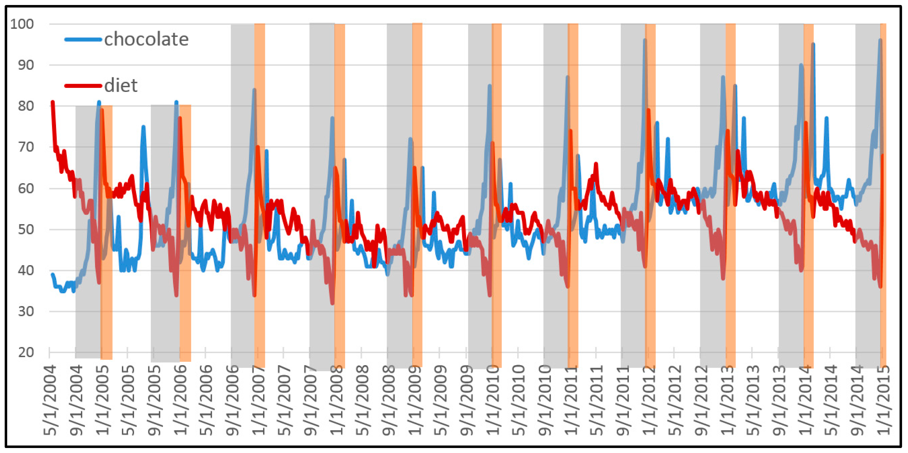
An illustrative example will help us to concretize the different steps that follow. Figure 1 shows the popularity of the Google search terms “chocolate” and “diet” between 2004 and 2015. This pattern is of great value for a company that specializes in a portfolio of related products. Over the entire decade, the population of both terms together has grown some 10.8%. This total growth can be explained in terms of varying growth rates of each term, and therefore in terms of natural selection between both types. Our first step consists in deriving a descriptive equation that decomposes this dynamic of natural selection into information theoretic metrics.

If we assume that global interest in both search terms is correlated with economic demand for related products, a data savvy entrepreneur should be able to exploit the pattern to maximize the growth of its business. This is done by endogenously allocating resources to optimally “ride the wave” depicted by this exogenously given pattern. If the entrepreneur has a crystal ball that perfectly gives away the future, the answer is easy: sell the product which is most in demand at each time. If there remains uncertainty about the pattern, the theory of bet-hedging tells us how to best manage the portfolio. Our second step consists in deriving this longstanding result from our descriptive equation of natural selection.

Our third goal in providing an intuitive explanation of this process in terms of a communication channel between the uncertain environment and the evolving population. It turns out that the search for optimal growth consists in the search for the mutual information (or unequivocal signals) between the environment and the evolving pattern. This requires insights about the environment (at least about the probabilities of its possible states). In today’s “big data” economy, the entrepreneur would employ a data analyst to provide this intelligence about the environmental pattern. Information theory allows us to quantify the gained information from such pattern and convert this information into a measurable input for growth. Information is a measureable input for growth: “this much information” equals “that much growth potential”.

The following first section will review the contribution of the article in light of the existing literature. It provides context, but skipping it will not affect the reader’s ability to follow the succeeding sections. The subsequent method section presents the information theoretic decomposition, shows how the setup allows to optimize growth, and shows its relation to several special cases that have been treated in previous literature. The subsequent results section applies the decomposition to two practical cases for illustrative purposes. One specifies the illustrative example from Figure 1 and the other one refers to the division of labor in the extraction of resources in the global economy. The final discussion section presents the limitations and discusses possible extensions of the model.

1.1. Relation to Previous Work

The following combines the results from three bodies of literature. Each one of them has strengths and shortcomings. The first one is linked to Fisher’s fundamental theorem of natural selection and uses information theoretic terms to describe growth, but assumes an unchanging environment. It has not been generalized to varying environments (Section 1.1.1. Evolutionary Economics: Decomposing Growth Descriptively The second one (Section 1.1.2. Portfolio Theory: Optimizing Growth) builds on the literature of bet-hedging and portfolio theory. It works with varying environments, but in order for the information theoretic metrics to appear in the equations it requires some kind of proactive strategy that hold population frequencies constant at each time step. It therefore does not describe natural selection, which changes population shares over time. The last one consists in a meaningful interpretation of the role of information in society. This has traditionally been the domain economic decision theory, which uses proxy metrics to quantify information, not information theory (see Section 1.1.3. Economic Decision Theory: Interpreting Information. This article presents a single approach that draws from and links these three approaches to information and growth.

1.1.1. Evolutionary Economics: Decomposing Growth Descriptively

Information theoretic metrics have recently been introduced to describe natural selection. The basic spirit follows a longstanding tradition of both evolutionary economists [17,18,19,20] and evolutionary population biologists [21,22,23] to decompose population growth into different metrics of diversity, usually variance and covariance terms (such as done by the famous Price equation). Our equations also decompose growth in a similar manner, but use diversity metrics like entropies and mutual information instead. This expands recent work that has shown that natural selection expressed through replicator dynamics can be reformulated in terms of relative Kullback-Leibler entropy $D_{KL}$ [24,25,26,27]. Especially Frank [28,29] has worked out a clear link between relative entropy and Fisher’s fundamental theorem of natural selection [30]. Instead of quantifying the strength of selection with the variance of fitness in order to describe (as proposed by Fisher) it is measured with the divergence of population frequencies before and after updating through selection: $D_{KL}(P^{+}\parallel P)$. Just like Fisher’s fundamental theorem only applies to an unchanging environment [23,31], this literature assumes that the fitness of types stays the same over the time of observation (an assumption known as the model of “pure selection” in evolutionary economics [32]. Our decomposition includes this relative entropy metric of the strength of selection as one of its four parts of our initial equation, but expands it to a multivariate joint relative entropy in order to describe evolution over varying environments.

1.1.2. Portfolio Theory: Optimizing Growth

Portfolio theory focuses on proactive strategies to optimize growth in varying environments. As early as 1956, the information theorist John Kelly suggested to optimize long term growth by endogenously adjusting the distribution of types in a population to an exogenously given environmental pattern [33] (for a clear review see [14]). This idea has grown several branches [34], and is known as portfolio theory [35,36,37,38,39,40], growth optimal investment [41,42,43], biological bet-hedging [44], mixed optimal strategies [45], or stochastic (phenotype) switching [46,47]. While Kelly originally worked with the limited case of a diagonal payoff matrix (one type per environmental state), his results have more recently been expanded to the general case of any kind of “mixed fitness matrix” [47,48,49,50]. The main result of this literature holds that fitness can be increased with information about the environment $E$ through a signaling cue $C$. Such cues can for example consist of a fine-tuned environmental pattern detected by a machine learning algorithm of a big data company or an economic cycle detected by econometric analysis. The obtained information is quantified with the mutual information between the two, which we will refer to as $I(E;C)$ (for a short introduction to the main metrics of information theory see Supplementary Section 1).

The related information theoretic reformulations require that population frequencies are held constant, which leads to an omnipresent assumption that resources are actively redistributed by some kind of portfolio manager (or stochastic switch on the genetic level). However, in many dynamics as they occur in nature and society, there is no omnipotent portfolio manager who orchestrates population change (e.g., see the example of Figure 1). There is just natural selection between types with different growth rates. Our decomposition allows to describe evolution through natural selection.

1.1.3. Economic Decision Theory: Interpreting Information

Most existing work that interprets the role of information in growth dynamics follows in the footsteps of economic decision theory [51,52], often with relation to game theory [53] and the creation of prices in a market [54]. Broadly speaking, decision theory defines information as the difference in payoff with and without information. For example, the value of information is equivalent to the economic value provided by distinguishing between a high-quality car and a “lemon” [55]. This measures information in US$, and therefore does not measure information, but its effects through some kind of ad hoc cost function. The metrics of information theory allow to quantify the involved amount of information directly in its natural metric: bits. Mathematically, both approaches are closely related and essentially hinge on the effects of a newly introduced conditioning variable [25,31,32]. We will provide a complementary interpretation of the role of information in evolving social populations. We interpret ‘fit-ness’ as the ‘informational fit’ between the evolving population and its environment. This occurs over an (often noisy) communication channel.

1.2. Main Contributions

The main contribution of this article consists in combining the information theoretic description of natural selection in varying environments with optimal population portfolios through bet-hedging. The key consists in working with the average state of the population during typical updating, a concept that has not been used in previous literature. This will then lead to a new metric, namely the mutual information between the (average) updated population and its environment, $I(G^{+};E)$. It arises from the optimization of natural selection through bet-hedging. It also lends itself to the intuitive explanations of growth as a communication process between the evolving population and its environment, and the ‘informational fit’ between both, and naturally extends to cases with side information, as previously explored by the bet-hedging literature.

1.2.1. Combining the Descriptive and the Optimal

As a first step, the article presents a generalization of pure selection models of natural selection in unchanging environments to an information theoretic description of growth in a stationary, but varying environments. It can be used as a descriptive tool. In terms of the following equations, our descriptive decomposition of growth in Equation (2) includes a multivariate relative entropy term of $D_{KL}(P^{+}\parallel P)$ that quantifies the strength of selection (an expansion of the results of [28,29]). When growth in a stationary environment is optimized through bet-hedged log-optimal portfolios, this term turns into the mutual information between the updated population and the environment $I(G^{+};E)$ (Equations (5) and (6)). If there are additional cues about the environment (Equation (11)), the result is the three way mutual information between the updated population, the environment, and the signaling cue: $I(G^{+};E;C)$. Since optimal growth implies that the population absorbs all the information between the environment and the cue during updating, the result is the special case of a Markov chain: $I(G^{+};E;C)=I(E;C)$. This links our results back to the well-established result from the literature of bet-hedging, which identified $I(E;C)$ as the key variable in optimized growth (in line with [47,48,50,56]).

1.2.2. Growth as a Communication Process

The newly introduced measure $I(G^{+};E)$ also lends itself to the intuitive interpretation of growth as a communication process between the updated population and its environment. Optimal communication over the communication channel is equivalent to optimal growth. The extreme case is a noiseless channel, which is Kelly’s original case [33] and sets the (often hypothetical) benchmark of optimal fitness. With the presence of a noisy channel, growth can be optimized by converting the natural selection’s relative entropy term of $D_{KL}(P^{+}\parallel P)$ into the mutual information between the population and the environment: $I(G^{+};E)$. The mutual information measures those signals that clearly and unequivocally stem from the environment. This allows the population to absorb all environmental structure during updating, resulting in what we detect as optimal growth.

The literature of bet-hedging then tells us that it is possible to increase growth by learning about the information patterns of the environment. This is exactly what big data companies aim at when analyzing patterns of shopping behavior to increase sales, investment banks when analyzing stock market patterns to optimize stock portfolios, and macroeconomic policy makers when designing industry subsidy schemes. Information becomes a quantifiable ingredient of growth optimization. Information theory allows us to go beyond the distinction of growth effects with or without information (as common in decision theory), but allows us to quantify how much information (in bits) leads to how much growth potential by analyzing the communication channel between the evolving population and its varying environment.

2. Method: Fitness as Informational Fit

The total population grows by reproducing in a varying environment. Different environmental states are represented by random variable with distribution $P(E)$. Our assumption of knowing $P(E)$ implies that we have access to the uncertainty in the environment, but that there remains risk as to the specific realization of this random variable: in a Knightian sense [57] we do not know for sure which environmental state will be next (Knightian risk), even so we know it occurs with a chance of x% (Knightian uncertainty).

The population is subdivided into different groups of population types $G$, with each group $g$ consisting of a certain number of individual units. For simplicity, possible types and environmental states are assumed to be discrete. The replicators could be genes and the groups $g$ alleles; of US$ and different types of industry; or number of employees and restaurant chains; or online clicks and videos, etc. The math is indifferent to the choice of the quantity that is changing over time. In this descriptive setup, all offspring units inherit the type $g$ from their parents. The growth factor is represented with $w=\frac{unitsattimet+1}{unitsattimet}$. If some groups grow faster than others, natural selection takes place.

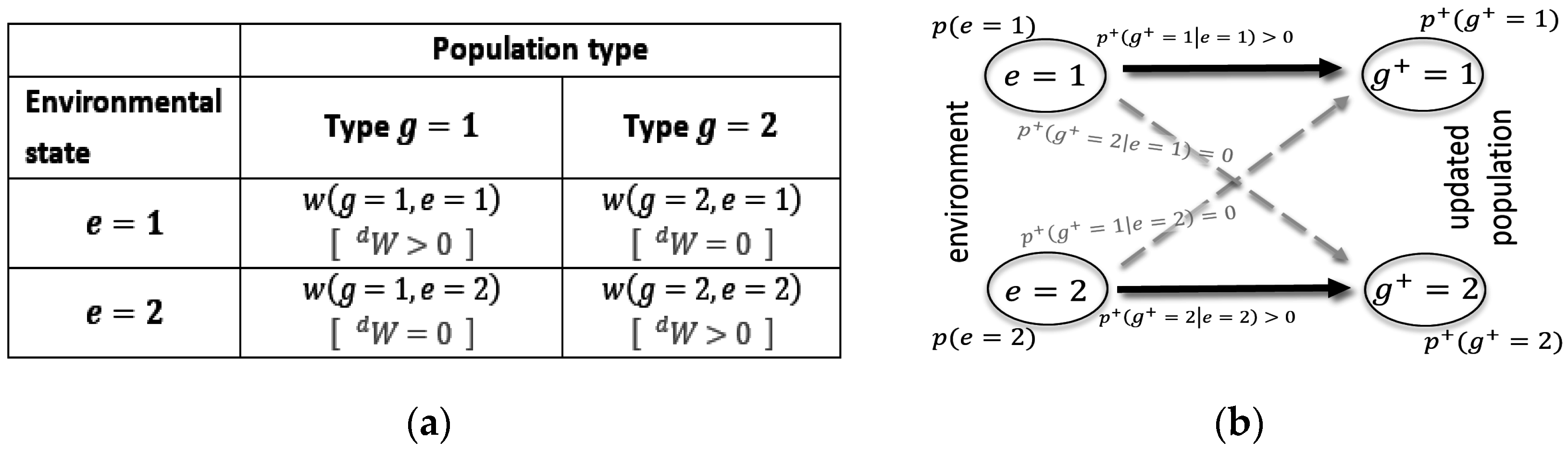
The growth factor of a specific group $w(g,e)$ depends both on the realization of its type $g$, and on the state $e$ of the environment $e$. This can be characterized by a traditional fitness matrix [58], such as the one illustrated in Figure 2a.

The single overbar represents the expectation over all type $g$ in a specific environment: $\overline{W}(e)=E_g\left[w(g,e)\right]$. We are interested in the long-term fitness over varying environmental states, which is given by the weighted geometric mean of the population fitness over all environmental states: $\stackrel{\overline{¯}}{W}={{\displaystyle \prod }}_e\overline{W}{(e)}^{p(e)}$. For empirical data, this average can be calculated even for a short and nonstationary time series, in which case $p(e)$ would reflect the proportional frequency of an environmental state during this period. Mathematically the following decompositions are still exact for this case. However, its information theoretic meaning derives from the assumption that the environmental pattern is stationary and ergodic, which converts the count of frequencies into reliable probabilities. In other words, in order to obtain information about the environment, there needs to be a reliable pattern in the environmental distribution. For example, the environment can consist of the typical set of an i.i.d. process, or be a deterministic periodic cycle such as day and night, or the four recurring seasons. It could also consist of any Markov process that convergences quickly enough to result in a unique stationary distribution. In this sense, the required time span of our evolutionary observation over $t=\left\{0,1,2,\dots .T\right\}$ depends on the reliability of the environmental pattern. In the asymptotic case where $T\to \infty$, we know that a stationary and ergodic Markov process will always converge.

We end up with two kinds of variables that can be empirically detected: the environmental distribution $P(E)$; and growth factors $w$ (overall population growth $\overline{W}(e)$, and type growth in an environmental state $w(g,e)$). In practice the latter can be detected as the respective geometric means conditioned on a certain environmental state. We can derive two additional variables: the average population shares before updating ($P$) and after average updating ($P^{+}$). In practice we calculate them as the average share $p(g|e)$ occupied by each type during a particular environmental state $e$. They are provided by solving for the weights of the mean fitness per environmental state $\overline{W}(e)={{\displaystyle \sum }}_g\mathit{p}(\mathit{g}|\mathit{e})*w(g,e)$. The so-called “replicator equation” [59] then defines the average population shares after average updating over the selected period of evolutionary observation: $p^{+}(g^{+}|e)=p(g|e)\frac{w(g,e)}{\overline{W}(e)}$. The superscript ⁺ indicates the average updated generation after reproduction (while no superscript refers to the average distribution before updating).

The result are the conditional distributions $P(G|E)$ and $P^{+}(G^{+}|E)$ derived from our empirically determined growth rates. They represent the average population distributions before and after average updating during the chosen period of growth observation. While these average distributions seem unfamiliar, they turn out to provide important insights. Through multiplication with the empirically detected environmental distribution, we obtain the respective joint distributions, e.g., $p(g|e)*p(e)=p(g,e)$ (note that $P(E)=P^{+}(E)$, as updating of the population does not change the distribution of the environment). In the following we will work with the resulting joint distributions between the environment and the population before and after average updating, $P(G,E)$ and $P^{+}(G^{+},E)$, with its conditionals, such as $P(G|E)$ and $P(E|G),$ and with its marginals, $P(G)$, $P^{+}(G^{+})$ and $P(E)$.

2.1. Decomposing Growth into Bits

Without loss of generality, the complete decomposition of long-term fitness is best represented on a logarithmic scale (which is customary in economics, for example). Logarithms of base 2 represent growth in terms of the number of population doublings at each time step, which at the same time quantifies the involved informational metrics in bits. The decomposition consists of four terms (for its derivation see Supplementary Section 2). The following section reviews each of them in turn.

Before getting into these details, the pseudo Equation (1) aims at providing the conceptual intuition. It says that the average growth of the population, is equal to the (usually hypothetical) benchmark of a noiseless channel between the environment and the population (expressed with a diagonal fitness matrix), minus the divergence between this hypothetical benchmark and reality (expressed with a Kullback-Leibler divergence), minus the remaining environmental uncertainty (conditional environmental entropy), minus the average strength of natural selection (a divergence before and after average replication of the population). Equation (2) uses the more exact notation that we will explore going forward.

$$\begin{gathered} \begin{array}{c}Average\\ growth\end{array}=\begin{array}{c}noiseless\\ benchmark\end{array}-\begin{array}{c}landscape\\ constraint\end{array}-\begin{array}{c}remainingenv.\\ uncertainty\end{array}-\begin{array}{c}directed\\ selection\end{array} \\ \left\{\stackrel{\overline{¯}}{W}\right\}=\left[{}^{diag}\cdot W\right]-D_{KL}(P^{+}\parallel {}^{diag}\cdot W)-H(E|P^{+})-D_{KL}(P^{+}\parallel P) \end{gathered}$$

(1)

$$\log \stackrel{\overline{¯}}{W}=E_e\left[{\log }^{d}W\right]-D_{KL}(P^{+}(e|g^{+})\parallel M(e|g))-H(E|G^{+})-D_{KL}(P^{+}(g^{+},e)\parallel P(g,e))$$

(2)

2.1.1. Benchmark of the Noiseless Channel

The first term on the right hand side of Equation (2) refers to the benchmark of noiseless communication channel between the environment and the updated population. It is the only positive term of the decomposition, and therefore defines maximal growth. The remaining three terms are all quantities that subtract from it (entropies are always nonnegative: $H\ge 0;D_{KL}\ge 0$ [14]). In this sense, growth is looked at in terms of a potential to achieve this (often hypothetical and illusive) benchmark of optimal growth.

As shown in Figure 2b, a noiseless channel means that the only valid transition is a direct transition (i.e., from state 1 to state 1, and from state 2 to state 2), while crossover noise (i.e., from state 1 to state 2 and vice versa) does not occur. The corresponding fitness matrix is a diagonal matrix, with all but one growth factor per environment being larger than 0. This is indicated by ${}^{d}W$ in Figure 2a. Kelly’s original results were obtained for such special matrixes [33]. Figure 2b also visualizes the insightful fact that in this case $P(G^{+})$ is exactly reflective of $P(E)$, which implies that the population distribution adopts to the environmental distribution during average updating.

As with most communication channels, also evolution’s communication channel is noisy, which in our case is due to the constraints of the existing fitness landscape. However, the noiseless channel sets the benchmark. Therefore, in most real-world cases, this first term of the noiseless channel is a hypothetical construct [45,47,49,50,56], which we note with ${}_{hyp}{}^{d}W$.

2.1.2. Constraint of the Mixed Fitness Landscape

The quantity $D_{KL}(P^{+}(e|g^{+})\parallel M(e|g))$ measures the divergence between the actual fitness matrix and the hypothetical diagonal fitness matrix of the noiseless channel. It is a constraint that arises when the real-world fitness matrix is not diagonal and the communication channel between the environment and the population is noisy. It is a relative entropy or Kullback-Leibler divergence [60], an unsymmetrical and nonnegative measure of informational divergence between two distributions, in this case $P^{+}(e|g^{+})$ and $M(e|g)$. $P^{+}(e|g^{+})$ can be calculated from the empirical data and asks about what the environmental distribution looks like from the perspective of the population after average selection. $M(e|g)$ arises from the proposal to use a hypothetical weighting matrix (here $M(E|G)$) to represents any non-zero fitness value as a weighted average of fitness values from the hypothetical diagonal fitness matrix ${}_{hyp}{}^{d}W$ [45,47,48,49,50,56]. In other words, it assumes a hypothetical world with one perfectly specialized type per environment (the noiseless channel) and proposes that any existing type fitness is a combination of those specialized fitness values. Saying it the other way around, $m(e|g)$ represents the ratio between the real type fitness $w(g,e)$ and its respective hypothetically optimal fitness: ${}_{hyp}{}^{d}W$: $w(g=i,e)=m(e|g=i)*{}_{hyp}{}^{d}W(e)$, where ${{\displaystyle \sum }}_{e}m(e|g=i)=1$. The further the real fitness landscape from the noiseless channel (the further the real fitness matrix from the diagonal matrix), the larger the corresponding Kullback-Leibler divergence. Roughly speaking, this implies that more homogeneous fitness landscapes increase this divergence (and subtract from optimal fitness).

2.1.3. Remaining Environmental Uncertainty

The next term in the equation quantifies the remaining uncertainty of the environment after average updating through the conditional entropy $H(E|G^{+})$. Entropy is a measure of uncertainty. In essence it quantifies the uncertainty when the probabilities of states are known, but not the particular sequence in which they occur. In our conditional form, it looks at the remaining uncertainty after natural selection. The information gain with respect to the unconditional uncertainty of the environment can be quantified in terms of the mutual information between the environment and the average updated population: $H(E|G^{+})=H(E)-I(G^{+};E)$ [13,14]. Inserting this expansion into Equation (2) provides Equation (3), which shows that this gained information contributes positively to population fitness. In general, the less uncertainty remaining after average updating (measured in bits), the more population growth can be obtained:

$$\log \stackrel{\overline{¯}}{W}=E\left[\log {}^{d}W\right]-D_{KL}(P^{+}\parallel M)-H(E)+I(G^{+};E)-D_{KL}(P^{+}\parallel P)$$

(3)

2.1.4. Directed Selection

The last quantity $D_{KL}(P^{+}(g^{+},e)\parallel P(g,e))$ measures the force of selection between the distribution of the original and the updated population in a varying environment. It quantifies the divergence that occurs during updating (it is an expected value of the (log) relative fitness of types: $D_{KL}(P^{+}(g^{+},e)\parallel P(g,e))=E_{g^{+},e}\left[\log (\frac{w(g,e)}{\overline{W}(e)})\right]$). This agrees with the result of Frank [28,29], who shows that $D_{KL}$ is related to the variance in the growth of types. However, first of all, it includes the environment, and is therefore a multivariate joint entropy. Secondly, in contrary to the variance in fitness, it has directionality, because $D_{KL}$ is an asymmetric divergence with $D_{KL}(P^{+}\parallel P)\ne D_{KL}(P\parallel P^{+})$ in general, with $D_{KL}=0$ only if $P^{+}=P$ [14,61]. In information theory, $D_{KL}$ is used to measure the inefficiency (in bits) of assuming one distribution, when using it to encode another true distribution. In Equations (1)–(3) it measures the inefficiency of still assuming the original distribution $P(g,e)$ when evolutionary updating has already produced the true (updated) distribution $P^{+}(g,e)$. Turning up as a negative term in Equations (1)–(3) this inefficiency constrains population fitness.

Equation (2) can be used to describe any kind of evolutionary change of discrete replicators in a varying environment. It does not require an intervening strategy, such as a portfolio manager. We will now derive the well-known equations from the bet-hedging literature by optimizing Equation (2). This is can be achieved by the evolving population though the (endogenous) adjustment of available resources to (exogenously given) environmental patterns.

2.1.5. Fitness Optimization

When the next environmental state is known, the best strategy consists in allocating all resources to the type with the highest (arithmetic) expected fitness, $ma{x}_e\left[E_g\left[w(g,e)\right]\right]$. A portfolio strategy provides optimal population growth when the exact future is not known, but when a stationary distribution of different possible environmental states is known, $P(E)$, while there is uncertainty with regard to which specific environmental states will turn up next [33,35,36,37]. This is achieved by identifying a certain population distribution $P(G)$ which is held constant despite alternating selective pressure during different environmental states. This implies that there is a proactive strategy that counteracts natural selection during updating. We will denote it with the subscript $({\dots }_s)$. In biology this strategy is often implemented by a genotype which maintains a so-called ‘stochastic switch’ that keeps stable population shares of phenotypes, counteracting selective pressure that changes the distribution of types [44,61]. This means that even if certain phenotypes increase their share in a particular environmental state (and actually increase their share temporally), their offspring will be genetically distributed according to the same distribution as they were at birth. In economic evolution, a conscious portfolio manager can redistribute gains and losses in a way that keep stable shares of types. This does not change the fact the share of some stocks increase and others decrease their share temporally in a particular environmental state (the portfolio manager has real gains and losses). However, bet-hedging implies that the new bets will be distributed according to the same distribution as they were initially. In practice this is done through constant redistribution from winning to loosing types.

As such, bet-hedging affects our metric of directed selection. In order to understand its role, it is useful to reformulate it according to the chain rule of relative entropy [14]:

$$D_{KL}(P^{+}(g^{+},e)\parallel P(g,e))=D_{KL}(P^{+}(g^{+})\parallel P(g))+D_{KL}(P^{+}(e|g^{+})\parallel P(e|g))$$

(4)

The fact that a bet-hedging strategy maintains a stable population distribution $P_s(G|e)$ for each environment $e$, leads to the fact that $P_s(E|g)=P(E)$ (see Supplementary Section 3). This replaces the last term with $D_{KL}(P_s^{+}(e|g^{+})\parallel P(e))$. The classical interpretation of $D_{KL}$ is an inefficiency when encoding one distribution (for former one in the parenthesis) with a code that is optimized for another distribution (the latter one). This interpretation suggests that $D_{KL}(P_s^{+}(e|g^{+})\parallel P(e))$ is the informational inefficiency that arises when the objective (unconditioned) environmental distribution is used to encode the distribution of the environment as it arises from the perspective of the updated population. Given the negative sign of the term (Equation (2)), this inefficiency limits the achievable growth rate and it will only disappear if the updated population perceives the environment ‘as it is’ ($P_s^{+}(e|g^{+})=P(e))$ (as for example possible with perfect foresight for the next environmental state).

There are many ways to hold a stable $P_s(G|e)$ for each environment $e$. Optimized bet-hedging does not simply look for any fixed type distribution but for a distribution that results in a fixed point in which the distribution before updating in every environment $P_s(G)$ is the same as the average distribution over all environmental states after updating $P_s^{+}(G^{+})$. In other words, fitness optimization searches for the fixed point at which the average population distribution is fixed in a varying environment despite natural selection.

This effectively eliminates $D_{KL}(P^{+}(g^{+})\parallel P(g))$ in Equation (2) and contributes to an increase in population fitness (due to the reduction of this negative term). This converts Equation (4) into: $D_{KL}(P_s^{+}(g^{+},e)\parallel P(g,e))=D_{KL}(P_s^{+}(e|g^{+})\parallel P(e))$. Expanding the latter term shows that it is equivalent to Shannon’s mutual information [13,14], which leaves us with the following equality for the case of optimal growth through bet-hedging:

$$D_{KL}(P_s^{+}(g^{+},e)\parallel P_s(g,e))=I(G_s^{+};E)$$

(5)

This means that our metric for directed selection turns into the mutual information between the environment and the average updated population. This then converts our original Equation (2), into Equation (6), which is equivalent to Equation (7) (since $H(E|G_s^{+})+I(G_s^{+};E)=H(E)$). Supplementary Section 4. shows that optimal growth always implies the equivalence relation of Equation (5). However, the revers requires that types are defined in a way that they are linearly independent in the fitness matrix (in a sense of linear algebra) and that environmental states are defined in a way that makes them linearly independent (among each other, in a sense of linear algebra) (Supplementary Section 4). This seems to be a reasonable demand, as redundant types can be merged, as well as redundant environmental states. Such independence is assured for Kelly’s original case, for which there is only one type that is perfectly adopted to one specific environment (a diagonal matrix).

$$\mathit{log}\stackrel{\overline{¯}}{W}=E_e\left[\mathit{log}{}^{d}W\right]-H(E|G_s^{+})-I(G_s^{+};E)$$

(6)

$$\mathit{log}\stackrel{\overline{¯}}{W}=E_e\left[\mathit{log}{}^{d}W\right]-H(E)$$

(7)

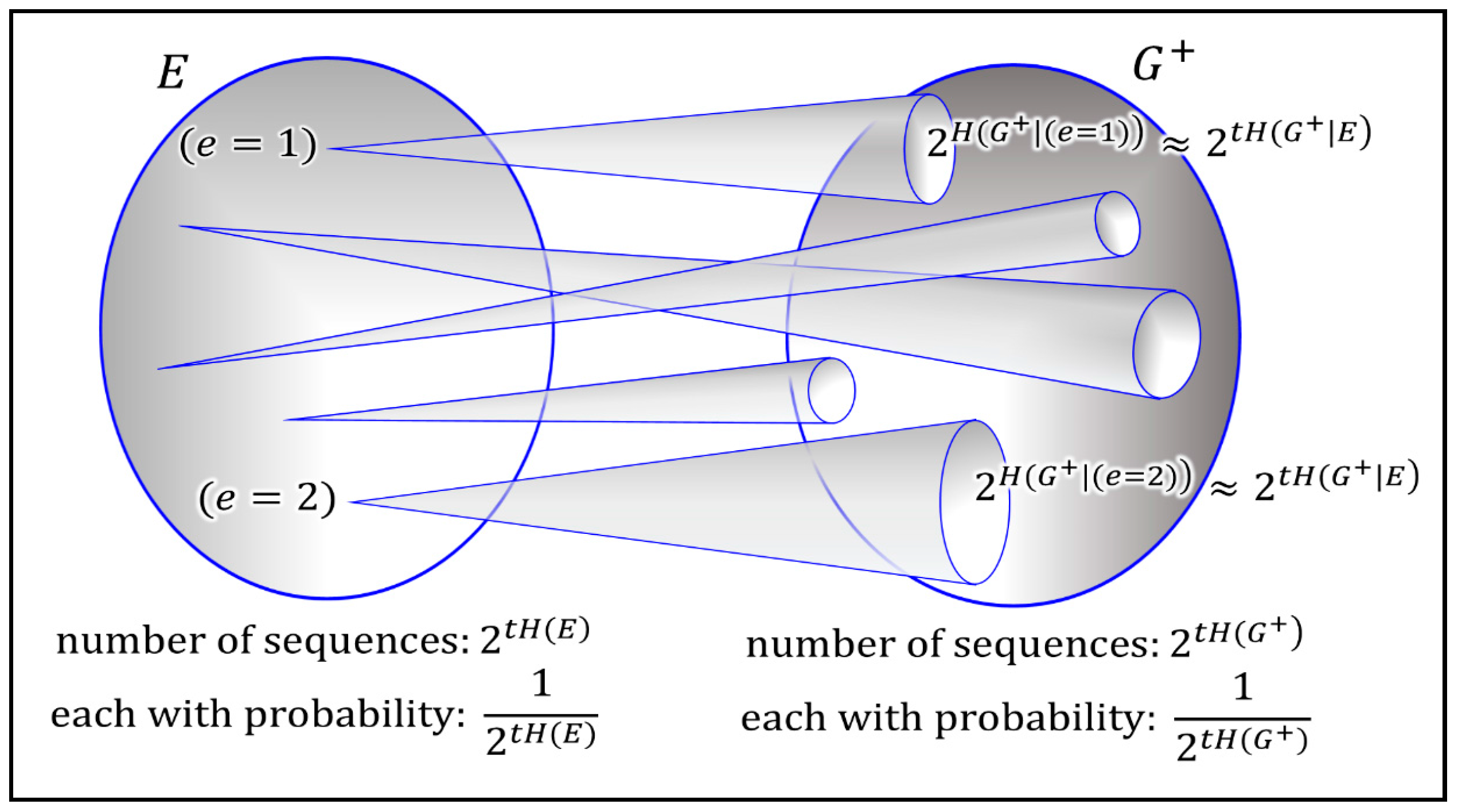
This result lends itself naturally to an interesting interpretation. The mutual information $I(G^{+};E)$ quantifies the amount of structure in the updated population $G^{+}$ that is assured to come from the environment $E$. This can be understood when interpreting mutual information in terms of a non-confusable input signals (see Figure 3). In information theory this is often explained with help of an analogy to a noisy typewriter (see the information theory primer of the Supplementary Section 1). The technical reasons is the nature of joint typicality of both sets (for a formal proof see any standard textbook on information theory [14,15]). The intuitive interpretation is that optimal growth implies that the population absorbs all useful structure obtainable from the environment.

2.2. Special Cases

The decomposition of Equation (2) is a generalization of several special cases that are well-known in the literature. They are listed in

Table 1. Comparison of the descriptive decomposition (Equation (2)) and its special cases (Equations (6)–(10).

Log of Population Growth	Noiseless Channel	Fitness Landscape Constraint	Remaining Environmental Uncertainty	Directed Selection
$\log \stackrel{\overline{¯}}{W}=$	$E_e\left[\log {}_{hyp}{}^{d}W\right]$	$-D_{KL}(P^{+}(e|g)\parallel M(e|g))$	$-H(E|G^{+})$	$-D_{KL}(P^{+}(g,e)\parallel P(g,e))$	Equation (2)
Kelly’s case no bet-hedging	$=E_e\left[\log {}^{d}W\right]$	+ 0	$-H(E)$	$-D_{KL}(P(e)||P(g))$	Equation (8)
Kelly’s case with bet-hedging	$=E_e\left[\log {}^{d}W\right]$	+ 0	$-H(E)$	+0	Equation (7)
optimal inside bet-hedging region	$=E_e\left[\log {}_{hyp}{}^{d}W\right]$	+ 0	$-H(E|G_s^{+})$	$-I(G_s^{+};E)$	Equation (6)
	$=E_e\left[\log {}^{d}W\right]$	+ 0	$+\mathbf{0}$	$-H(E)$	Equation (7)
stable shares outside bet-hedging region	$=E_e\left[\log {}^{d}W\right]$	$-D_{KL}(P_s^{+}(e|g)\parallel M(e|g))$	$-H(E)$	+ 0	Equation (9)
optimal with perfect cue	$=E_e\left[\log {}^{d}W\right]$	$-D_{KL}(P_s^{+}(e|g)\parallel M(e|g))$	$+0$	$+0$	Equation (10)

.

2.2.1. Kelly’s Setup

The most well-known special case refers to Kelly’s interpretation of information rate [14,33]. Kelly’s criteria has also been the main lead in the search for the presented decomposition, as it shows the long-term superiority of bet-hedging strategies in the special case of a diagonal fitness matrix ${}^{d}W$. In this case Equation (2) simplifies to Kelly’s well-known result:

$$\log \stackrel{\overline{¯}}{W}=E_e\left[\log {}^{d}W\right]-H(E)-D_{KL}(P(e)\parallel P(g))$$

(8)

Kelly used this result to show that with a diagonal fitness matrix, population growth can be optimized through a proportional bet-hedging strategy that assures that the distribution of the population exactly matches the environmental distribution $P(E)=P_s(G)$, which sets $D_{KL}(P(e)||P_s(g))=0$ (see Table 1). In reference to the channel optimization (Equation (6)), this implies that the mutual information is equal to the plain entropy of the environment, which maximizes the mutual information: $\max I(G^{+};E)=H(E)$. This brings us back to the previously derived Equation (7). Shannon referred to the maximum of the mutual information $I$ as the “channel capacity”, the upper bound on the rate at which information can be reliably transmitted over a communication channel [13]. Naturally, in the best case, this maximum is achieved with a noiseless channel. So if additionally the dynamic of the future environment is known entirely and there is no environmental uncertainty, $H(E)=0$, the achievable growth rate consists of the benchmark case of the noiseless channel: $\log \stackrel{\overline{¯}}{W}=E_e\left[\log {}^{d}W\right]$ (compare with Equation (7)).

2.2.2. Non-Diagonal Fitness Matrices

Kelly’s winner-takes-it-all fitness matrix has been generalized to non-diagonal fitness matrixes [45,48]. In this case the benchmark of the noiseless channel refers to a hypothetical fitness matrix ${}_{hyp}{}^{d}W$ [47,49,50]. Proportional bet-hedging also achieves optimality, but the proportionality between the environmental distribution and the optimal population distribution is distorted by the shape of the fitness landscape.

As illustrated clearly in [48,50], this distorted bet-hedging works only within a certain range of population constellations, which has been termed the “region of bet-hedging”. Inside the region of bet-hedging it is possible to adjust the bet-hedging strategy to the distortion of the non-diagonal fitness landscape, setting the fitness landscape constraint to zero (see Equations (6) and (7) in Table 1). Our decomposition reveals that this is done by equating the hypothesized weighting matrix $M(E|G)$ with the stochastic matrix $P^{+}(E|G^{+})$. Outside the region of bet-hedging, optimization might suggest a negative value for $p(g)$. Negative investment (betting against a type) might make sense for selected applications to the stock market or gambling but does not straightforwardly generalize to any kind of bet-hedging strategy (such as product portfolios of a company, or biological evolution). Here we have to compute optimal bets subject to constraints that no bet is negative, which usually leads to the exclusion of certain types in the strategy.

Outside the region of bet-hedging, the achievement of full channel capacity is compromised by both the mismatch with the optimal diagonal fitness matrix and the uncertainty about the environment $H(E)$. This results in Equation (9).

$$\log \stackrel{\overline{¯}}{W}=E_e\left[\log {}^{d}W\right]-D_{KL}(P_s^{+}(e|g)\parallel M(e|g))-H(E)$$

(9)

2.2.3. End Result of Selection in Stationary Environments

Without an intervening portfolio strategy, the asymptotic end result of an endless time series $T\to \infty$ would assure that the type with the highest average fitness over all different environmental states dominates the population. This implies $p_s^{+}(e,g=fittest)=1$. Betting all resources on one type is also often the result of optimization outside the region of bet-hedging. It is insightful to note that in this case the uncertainty of the environment increases $\mathrm{H}(\mathrm{E}|G^{+})\to H(E)$ (see Equation (9) in Table 1), which implies independence between the resulting population and the environmental patters, $I(G^{+};E)=0$.

2.2.4. Perfect Foresight

The last case in Table 1 shows that the environmental uncertainty can be eliminated with a perfect signaling cue that completely describes the dynamic of the unfolding environment (Equation (10)). A perfect cue absorbs all environmental uncertainty. The consequent strategy simply places all weight on the type with the highest fitness. However, it is still constraint by the existing fitness landscape. Our empirical analysis shows that this can turn out to be an important impediment.

$$\log \stackrel{\overline{¯}}{W}=E_e\left[\log {}^{d}W\right]-D_{KL}(P_s^{+}(e|g)\parallel M(e|g))$$

(10)

2.3. The More Populations Know, the More They Can Grow

The former results are naturally extended to the situation that populations can use environmental signals by actively sensing the environment. These results also go back to Kelly [33]. Additional side information can be obtained either through observations of the past that influence current and future dynamics (‘memory’) or observations of third events that correlate with current and future dynamics (‘cues’) (for a systematic treatment between the differences of both, see [47,62]). In general, this introduces a new conditioning variable $C$. Conditioned on the realization of this side information, the joined distributions can change and we end up with fine-tuned strategies for each conditioned case.

It is a fundamental theorem in information theory that “conditioning reduces entropy” [14], and therefore communicates information. In Kelly’s setup it reduces environmental uncertainty through $H(E)\ge H(E|C)$, and therefore increases the achievable fitness in Equation (2). The increase is equal to the mutual information between the cue and the environment: $H(E)-H(E|C)=I(E;C)$, which has been termed the “fitness value of information” [47,48,50]. It is an upper bound for the potential increase in growth that can be obtained from the cue. Note that the value of information is independent from the fitness values $w(g,e)$.

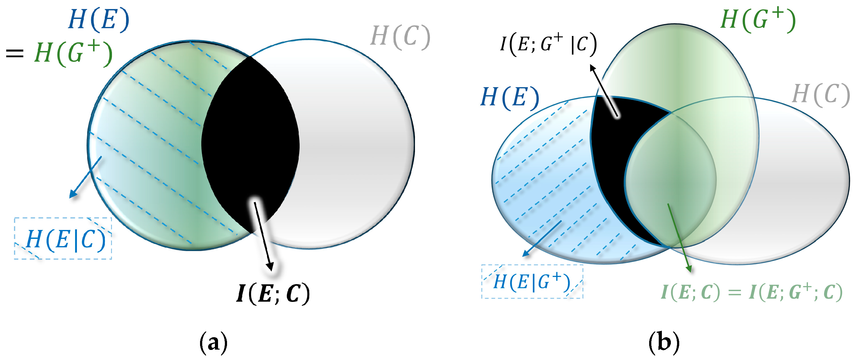
The following reveals how this relates to our descriptive approach of Equation (2). The argument requires a bit of information theory, but essentially links the mutual information between the environment and the signaling cue, $I(E;C)$, with the mutual information between the updated population and the environment, $I(G_s^{+};E)$ from Equation (5). A quite intuitive interpretation of this link follows the visual representation of mutual information as the overlapping intersection in the form of the Venn diagram, such as shown in Figure 4a (also called I-diagrams [14,15,63,64]. In this representation the circles are entropies $H$, and the intersections mutual information $I$.

In Kelly’s case of a diagonal fitness matrix, the distribution of the environment and the average updated population are a perfect match, with $H(E)=H(G^{+})$ (see Figure 4a). This hides the importance of the variable $G^{+}$ that emerged as a crucial variable in our descriptive decomposition. It turns out that in the case of optimal growth in non-diagonal fitness landscapes the three variables form a Markov chain $E\leftrightarrow G_s^{+}\leftrightarrow C$, where the cue and the environment are conditionally independent given the average updated population (see Figure 4b). In information theoretic terms this means that there is no mutual information between the cue and the environment given the updated population: $I(E;C|G_s^{+})=0$. In other words, optimal growth implies that all structure is absorbed by average updating during optimal growth. This leads to a conditional version of Equation (6):

$$\log {\stackrel{\overline{¯}}{W}}_{s|c}=E_e\left[\log {}_{hyp}{}^{d}W\right]-H(E|G_s^{+})-I(G_s^{+};E|C)$$

(11)

The fitness value of the cue is obtained by the difference between the fitness without cue (Equation (6)) and with cue (Equation (11)). Both the expected value term and the entropy term cancel and we obtain the three-way mutual information between all three variables: $\log {\stackrel{\overline{¯}}{W}}_{s|c}-\log {\stackrel{\overline{¯}}{W}}_s=-I(G_s^{+};E|C)+I(G_s^{+};E)=I(G_s^{+};E;C)$ (Figure 4b). It is important to notice that in principle three-way information can be negative [14,15,63,64], which would imply that additional information could decrease growth potential. However, since in our case $I(G_s^{+};E;C)=I(E;C)$ and since two-way mutual information is always nonnegative, Markovity assures non-negativity (this is visualized by Figure 4 and can formally be shown with the data processing inequality [14]).

The mutual information between the environment and the cue $I(E;C)$ is the main result for the fitness value of information [47,48,50,56]. From the perspective of our derivation, it turns out that this is a special case of the multivariate mutual information $I(G_s^{+};E;C)$.

3. Results: Empirical Applications

One of the main benefits of our descriptive decomposition is that it can readily be applied to analyze empirical time series. We do this now for two cases to obtain a feeling for the orders of magnitude of the different components and their trade-offs. It is important to emphasize that the idea of the following applications is not to study or learn anything new about the two chosen cases. The idea is not to study the behavior of the case’s subjects, but rather the behavior of our equations when applied to data. Some economically rather implausible aspects of the following cases will also clearly expose the limitations of underlying assumptions and point to a future research agenda.

The practical application of the presented decomposition is straightforward for the binary case with two types, as this allows to unambiguously identify the time average population shares from the empirically detected growth rates (multivariate cases require nonlinear constrained optimization). With all growth rates $w$ known, the binary case can be solved for $p(g_1|e)$ through:

$$\overline{W}(e)=p(g_1|e)*w(e,g_1)+\left[1-p(g_1|e)\right]*w(e,g_2)$$

(12)

3.1. Global Resources: Informing Division of Labor

One possible application refers to the division of labor between different economic agents. We take “the global use of materials since the beginning of the 20th century” according to the publicly available dataset [65,66]. This provides the evolution of global resource extraction for the 99 years between 1900 and 1998. Population growth $\overline{W}$ tracks the growth of global resource extraction in tons, including all biomass, fossil fuels, ores and minerals. Our two types $G$ of this global social organism distinguish between United States and the rest of the world. The more resource extraction, the more growth of the type, the fitter the type. We ask: how much could a bet-hedging strategy between the US and the rest of the world have increased the global growth of resources simply by exploiting stationary informational patterns of the environment?

Figure 5 shows that the type ‘United States’ extracted between 14% and 29% of total resources over the century. Global resource extraction grew with an empirical population fitness of $\stackrel{\overline{¯}}{W}=2^{0.02803}=1.962\%$ per year (

Table 2. Decomposition of global resource extraction between 1900 and 1998 into different cases. $H,D_{KL}$ and $I$ measured in bits.

	$\mathbf{log}\stackrel{\overline{¯}}{\mathit{W}}$	=	${\mathit{E}}_{\mathit{e}}\left[\mathbf{log}{}_{\mathit{h}\mathit{y}\mathit{p}}{}^{\mathit{d}}\mathit{W}\right]$	$-{\mathit{D}}_{\mathit{K}\mathit{L}}({\mathit{P}}^{+}(\mathit{e}|\mathit{g})\parallel \mathit{M}(\mathit{e}|\mathit{g}))$	$-\mathit{H}(\mathit{E}|{\mathit{G}}^{+})$	$-{\mathit{D}}_{\mathit{K}\mathit{L}}({\mathit{P}}^{+}(\mathit{g},\mathit{e})\parallel \mathit{P}(\mathit{g},\mathit{e}))$
Equation (2) descriptive	0.02803	=	1.02702	− 0.00005	− 0.99873	− 0.00021
Equation (6) optimal inside bet-hedging region	0.02822	=	1.02702	+ 0	− 0.99867	$-I(G_s^{+};E)$ − 0.000123
Equation (11) bet-hedging with cue WW2 in b-h region	0.02823	=	1.02702	+ 0	− 0.99867	$-I(G_s^{+};E|C)$ − 0.000111

). We now ask for an environmental patterns. One straightforward pattern identifies during which periods the relative fitness of one type is higher than in the other. In this case, the U.S. growth factor is superior in 51 of the 99 periods, resulting in $p(e=USfavorable)=0.52$. We can now obtain the average fitness values for each environmental state from our time series (calculating the respective geometric mean during each occurrence of the state), and calculate the average population shares of both types before and after updating (solving Equation (12) and using the replicator equation).

Assuming that the identified environmental pattern and type fitness are stationary, this information can be used to optimize population fitness by converting our directional selection term $D_{KL}(P^{+}(g,e)\parallel P(g,e))$ into the mutual information $I(G_s^{+};E)$ (drawing on Equation (5)). For practical purposes it is useful to remember that optimization implies the following conditions: $p_s(g)=p_s^{+}(g)$ and $p_s(e|g)=p(e)$. As shown in Supplementary Section 4, this implies a time-average of relative fitness equal to 1: $E_e\left[\frac{w(g,e)}{\overline{W}(e)}\right]=1$. In practice it is useful to solve for this condition.

Solving for this suggests that growth in this case can be optimized through bet-hedging, which offers a fitness value of ${\stackrel{\overline{¯}}{W}}_s=2^{0.02822}$ per year, or a compound annual growth rate of about $1.975\%$ (Table 2). The corresponding increase in fitness of ${\stackrel{\overline{¯}}{W}}_s-\stackrel{\overline{¯}}{W}=0.014\%$ is the “fitness value of the information” contained in the identification of the environmental distribution. This optimized population fitness is obtained if the share of the United States is held constant at $10\%$ throughout the century (through constantly bet-hedged resource redistribution between the U.S. and the rest of the world).

We now ask how side information about environmental patterns could have been used to improve the effectiveness of resource extraction in the global economy. Keeping things simple, we can test what will happen if we recognize that the century could reasonably be divided into two broad periods: pre- and post the end of World War II in 1945. It might not require a big data deep learning algorithm to hypothesize a meaningful distinction between these two conditions, but conditioning on these two periods already provides information (“conditioning reduces uncertainty” [14]). We optimize the channel throughput for each of these periods.

The left-hand side of the last two rows in Table 2 shows that conditioning increases fitness to ${\stackrel{\overline{¯}}{W}}_{s|c}=2^{0.02823}=1.976\%$ per year. In other words, the fitness value of recognizing the simple informational cue of the end of World War II provides the potential to obtain ${\stackrel{\overline{¯}}{W}}_{s|c}-{\stackrel{\overline{¯}}{W}}_s=2^{0.02823}-2^{0.02822}=0.001\%$ of additional fitness. This optimization is achieved by holding the share of the U.S. stable at $20\%$ before 1945, and at a stable $1\%$ afterward.

The right hand side of the last two rows in Table 2 reveals that this is achieved by obtaining a very small amount of information, namely: $-I(G_s^{+};E|C)-(-I(G_s^{+};E))=-0.000111+0.000123\approx 0.000012$ bits (compare Figure 4b for a visualization of this calculation; notice that $D_{KL}(P^{+}(e|g)\parallel M(e|g))=0$, as the results lie within the area of bet-hedging for all periods). While this fitness gain does not seem like much at first sight, it is equivalent to some 700 million additional tons of resources during the period compared to the empirical trajectory. The detected information bits are what enables this increase in growth potential in a stationary fitness landscape. Informational bits (right-hand side of our equation) converts to growth (left-hand side).

3.2. Big Data: Informing Business Growth Strategies

The second example return to the examples with which we motivated our exploration in Figure 1. It refers to a typical big data application in the economy, where growth is obtained by adjusting to detected environmental patterns. Figure 1 shows the Google Trends data for the search engine terms “chocolate” and “diet” from May 2004 to February 2015. The search behavior shows a clear pattern. Similar Google Trends patterns have proven to have significant correlations with a large variety of aspects in commerce, including stock market movements [67], trading behavior [68], automobile sales [69], company evaluations [70], and private consumption [71].

An entrepreneur selling both chocolate and diet products can exploit a natural complementarity of both trends over time. For reasons of tractability, we simply assume a one-to-one relationship between the normalized Google search trends and possible sales of chocolate and diet products by a big data savvy entrepreneur. This suggests that it is possible to sell an average of 106 products per week. The time series does not show a growth tendency (average weekly growth factor of exactly 1.0 over the 560 weeks, resulting in $\log (\stackrel{\overline{¯}}{W}=1.0)=0$,

Table 3. Exploration of different cases of the growth of Google Trends data for the search engine terms “chocolate” and “diet” from May 2004 to February 2015.

	$\mathbf{log}\stackrel{\overline{¯}}{\mathit{W}}$	=	${\mathit{E}}_{\mathit{e}}\left[\mathbf{log}{}_{\mathit{h}\mathit{y}\mathit{p}}{}^{\mathit{d}}\mathit{W}\right]$	$-{\mathit{D}}_{\mathit{K}\mathit{L}}({\mathit{P}}^{+}(\mathit{e}|\mathit{g})\parallel \mathit{M}(\mathit{e}|\mathit{g}))$	$-\mathit{H}(\mathit{E}|{\mathit{G}}^{+})$	$-{\mathit{D}}_{\mathit{K}\mathit{L}}({\mathit{P}}^{+}(\mathit{g},\mathit{e})\parallel \mathit{P}(\mathit{g},\mathit{e}))$
Equation (2) descriptive	0	=	0.98474	− 0.00074	−0.98207	− 0.00193
Equation (6) optimal in bet-hedging region	0.00229	=		+ 0	− 0.98073	$-I(G_s^{+};E)$ − 0.00173
With cue Sept-Dec.	0.00554	=		− 0.00154	− 0.97718	− 0.00048
With cues Sept-Dec. & Jan.	0.00987	=		− 0.00783	− 0.96703	+ 0
Equation (10) optimal with perfect cue	0.07421	=		− 0.91053	+ 0	+ 0

). We ask: how much can this entrepreneur potentially increase sales by simply exploiting a certain environmental pattern?

A straightforward environmental pattern $P(E)$ can again be detected by simply counting during which periods chocolate products sales grow faster than diet product sales (323 out of 559 weeks): $p(e=choc)\approx 0.58$. This informational pattern can already be used to optimize fitness. In environmental periods that favor the growth of chocolate products, chocolate products grow with a compound weekly growth factor of $w(g_{choc},e_{choc})\approx 1.05$, while diet products decrease with weekly $\approx 0.96$. In environments that favor diet products, those grow with $\approx 1.06$, while chocolate products decrease with about $\approx 0.94$.

Converting our directional selection term $D_{KL}(P^{+}(g,e)\parallel P(g,e))$ into the mutual information $I(G_s^{+};E)$ suggests that growth can be optimized by keeping a stable average share of chocolate products of roughly $66.8\%$ throughout the entire period of 559 weeks. As shown in the second row of Table 3, adopting this strategy increases growth by a value of $2^{0.00229}\approx 0.16\%$ of additionally obtainable compounded weekly growth. The corresponding strategy allows the entrepreneur to increase sales to an average of 177 products per week (Figure 6).

A closer look at the patterns in Figure 1 reveals the intuitively pleasing insight that chocolate leads over diet during the months of September to December (again, no artificial intelligence might be needed here). This suggests to fine-tune the strategy by introducing a conditional case that distinguishes between these different seasons. One strategy aims at the period from September to December, the other one from January to August (implementing Equation (11)). Table 3 shows that the growth value of this side cue information is equal to 0.38% (average 202 products per week). The optimization for this case turns to be outside the region of bet-hedging for the environmental state of “Sept.–Dec.”, but inside for “Jan.–Aug.”. As a result, the respective version of our decomposition in Table 3 contains both $D_{KL}(P^{+}(e|g)\parallel M(e|g))$ and $D_{KL}(P^{+}(g,e)\parallel P(g,e))$.

An even closer look at the data pattern reveals that diet products peak in January, right after the peak of chocolate products in December. This insight can be exploited by the entrepreneur by setting up a separate strategy for January. The optimization of the resulting three way partition of the year allows to obtain a weekly growth factor of 0.69% above the empirical growth rate, selling some 261 products per week. The last case in Table 3 refers to perfect information, which eliminates environmental uncertainty (per definition, with $H(E|G^{+})=0$). In this case the entrepreneurs know at each week with certainty which product will sell better and will simply focus on the better selling one.

Comparing the constituents of these last two cases in Table 3 reveals that any attempt to get closer to the unattainable benchmark of the noiseless channel confronts a trade-off between environmental uncertainty and the constraints of the non-diagonal fitness matrix. Optimization with ever better environmental signals reduces the remaining environmental uncertainty $H(E|G_s^{+})$, but also puts more weight on the fitness landscape constraint $D_{KL}(P_s^{+}(e|g)\parallel M(e|g))$. The reduction of environmental uncertainty comes at the cost of dealing with the constraints of the existing fitness matrix, which poses a limitation that cannot be overcome with more information about the environmental pattern alone.

4. Discussion

The presented decompositions come with several (sometimes subtle) assumptions. First and foremost, most currently existing information theory is based on the notions of stationarity and ergodicity. It assures that the involved typical sets of probabilities emerge. The distinction between mere proportional frequencies and true probabilities is in some cases less delicate than in other cases. Equation (2) could still be applied to a non-stationary dataset, with the limitation that $p$ would refer to empirically detected proportions (frequencies) not true probabilities. The resulting metrics would not truly be entropies, but merely metrics of diversity and evolutionary selection. While this rather seems like semantics, however, fitness optimization in Equations (5)–(11) requires the stationary continuance of the fitness matrix. Only if the environmental patterns are unchanged and only if the geometric means of type fitness stay unchanged can we exploit them through optimization [72]. Big data driven pattern recognition can only provide useful insights if the environmental patterns stay the same. If the patterns change, the model based on previous data (and therefore the resulting strategy recommendation) cannot explain the new pattern [73]. No stable patterns, no straightforward exploitation of the pattern.

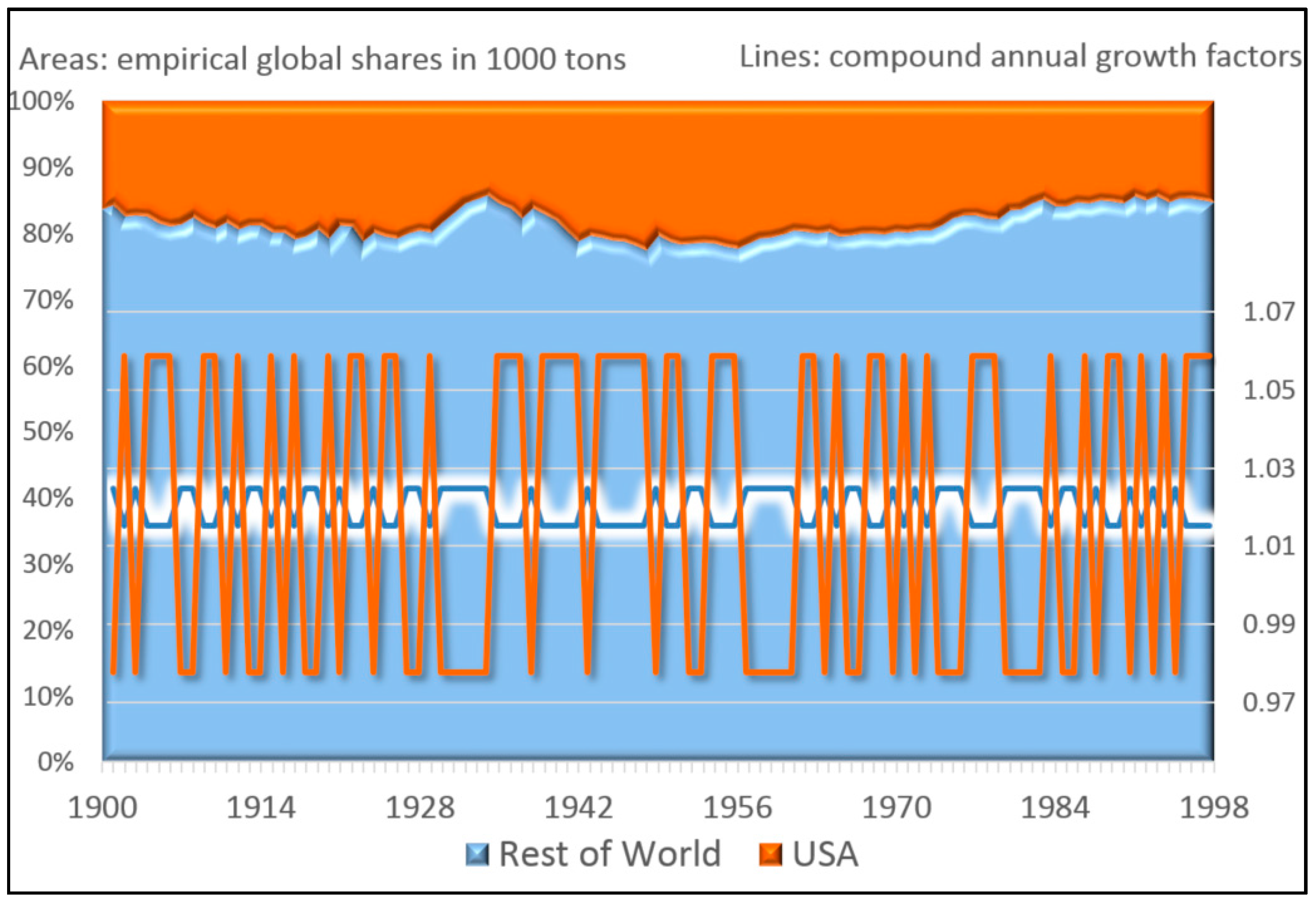
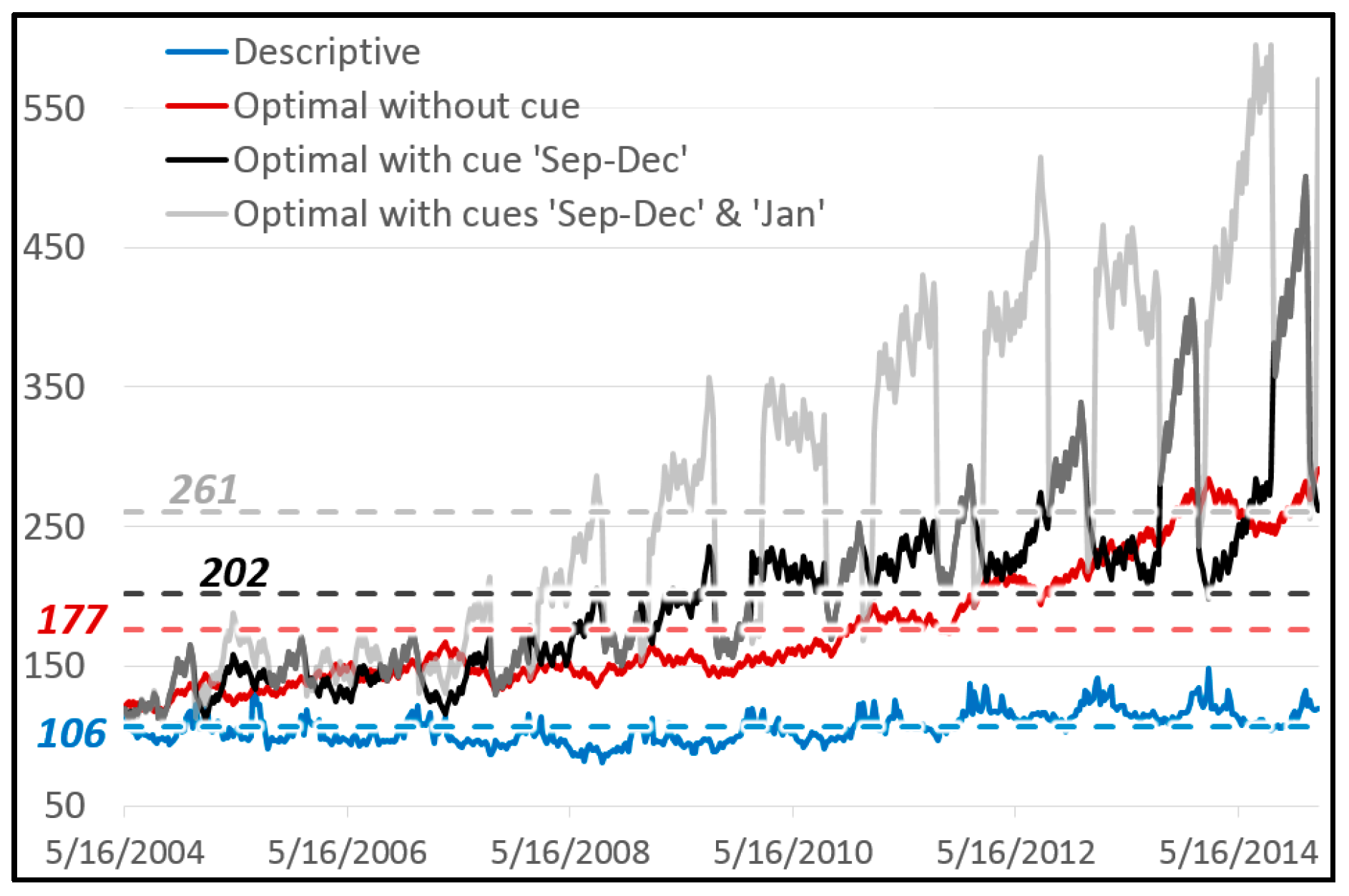
In reality, economic agents often influence and change environmental patterns as they evolve, destroying stationarity [74]. For example, the last equation in Table 3 suggests that a perfect cue would allow the big data entrepreneur to sell over 300 trillion products in the week after the observed 560 periods (instead of the empirically detected 106). Today the world only consumes around 125 trillion grams of chocolate per week. So there would certainly be no demand for as much chocolate. The existing environmental patterns and geometric mean fitness values would be changed endogenously, because density dependence would quickly reach the carrying capacity of the environment [72].

The idea of density dependence is well explored in the traditional theories of evolutionary economics and growth, but yet lacks a formal equivalent in terms of information theory. This does not mean that information theory does not provide the tools for exploring it. Actually, information theory can be used to identify change points in endogenous and exogenous dynamics [75]. It can also be used to model a truly bidirectional communication between the growing population and its environment. Cherkashin, Farmer and Lloyd showed that in the case of feedback between the environment and the population, the optimal bet-hedging strategy depends on the particularities of their mutual influence [76].

Another rather quite subtle assumption consists in the fact that we need a meaningful way to partition the evolving population to create the types of variable $G$. The chosen partition influences the calculated informational quantities. This leads to the fundamental question of how to best structure a growing population. What it is that evolves? This requires to identify a meaningful taxonomy of levels of types [77]. In the evolution of social system this is often not as obvious as in biological evolution.

There are several additional assumptions that have already been explored in the literature for the special case of fitness optimization through bet-hedging. Since our descriptive Equation (2) naturally link to the Kelly’s bet-hedging ansatz (Equations (8)–(11)), it is straightforward to relate the here presented descriptive decomposition to these extensions, including the consideration of the cost of information [61], multiple sources and series of frequent cues [62], decentralized and noisy signals [47,78], and the extraction of physical energy [79].

Summing up, recasting the dynamics of evolutionary population dynamics in terms of information theory has two ends. First, the arising communication channel between the growing population and its environment leads to straightforward, intuitive and meaningful interpretations. Information theory provides formal metrics for uncertainty ($H$), uncertainty reduction ($H(.|.)$) and the fit between the economic and environmental patterns (like $D_{KL}$ and $I$). This allows for a straightforward interpretation of the role of information in our information age. The more information is obtainable by economic agents about environmental patterns, the better can they assure that there is an “informational fit” between the environment and the growing population, which implies higher “fit-ness” or growth. Information itself becomes a quantifiable ingredient to exploit growth potential.

Second, it allows to create a formal link between the role of information in the dynamics of natural selection and in fields like engineering, computer science, statistical mechanics, and physics. Linking our descriptive decomposition of natural selection to the established results from portfolio theory, we can see that the role information plays in growth is similar to the role it plays in the physical relation between information and energy [79,80,81,82]. A longstanding body of literature in physics going back to the late 19th century has shown that information can be seen as the equivalent to the potential to do work. The workhorse for this relation in physics is Maxwell’s demon [83], who uses information about its environment to extract energy from it [84,85,86]. Much like the demon converts information into the potential to do physical work, economic agents can use informational patterns to increase their potential to grow (for an analogy between bet-hedging and Maxwell’s demon see [79]). This provides ample potential for cross-fertilization among complementary interpretations of the formal conceptualization of information and its role in growth.