Formulation of Exergy Cost Analysis to Graph-Based Thermal Network Models

Abstract

Information from exergy cost analysis can be effectively used in the design and management of modern district heating networks (DHNs) since it allows to properly account for the irreversibilities in energy conversion and distribution. Nevertheless, this requires the development of suitable graph-based approaches that are able to effectively consider the network topology and the variations of the physical properties of the heating fluid on a time-dependent basis. In this work, a formulation of exergetic costs suitable for large graph-based networks is proposed, which is consistent with the principles of exergetic costing. In particular, the approach is more compact in comparison to straightforward approaches of exergetic cost formulation available in the literature, especially when applied to fluid networks. Moreover, the proposed formulation is specifically considering transient operating conditions, which is a crucial feature and a necessity for the analysis of future DHNs. Results show that transient effects of the thermodynamic behavior are not negligible for exergy cost analysis, while this work offers a coherent approach to quantify them.

1. Introduction

Thermoeconomics is a rational approach for understanding the process of cost formation within energy systems. This process is based on the way of using energy resources according to their quality, the latter being expressed through the concept of exergy. Thermoeconomics can be applied to energy systems with different purposes: costing [1], design improvement [2], optimization [3], diagnosis [4], control [5], etc.

Since thermoeconomics is a thermodynamic-based costing method, it is highly interesting for the evaluation of district heating networks which involve the use of both thermal and mechanical energy [6]. In [7], authors highlight the usefulness of low-temperature integration to increase the district heating network’s (DHN) performance and reduce friction losses. Due to the fact that system performance of DHNs is highly related to thermal losses and the temperature levels in the network, thermoeconomics seems to be a reasonable way of accounting for them. A survey of actual literature clearly shows that this approach is used for the design of DHN systems [8], calculation of optimum pipe insulation thickness [9] and performance assessment of renewable supply [10]. Cost accounting based on exergy is particularly useful to evaluate the primary energy savings associated with retrofitting options applied to buildings connected with district heating [11] or to compare the production costs of different producers depending on their position and the quality of their heat produced [12]. These are important aspects in modern district heating networks, where it is crucial to take advantage of heat available from industrial processes, renewable energy or local resources. In addition, exergy costing could be a rational basis for regulating third party access to the heating infrastructure. Thermoeconomic analysis can be also used for helping heuristic optimization procedures, as proposed in [13], where a simulated-annealing algorithm has been applied to DHN planning.

In order to improve the DHN performance both in design and operation, the representation of such networks based on graph theory seems promising. This model approach was developed in [14] and is based on graph theory topology and a time-dependent, thermo-fluid dynamic solving technique to analyze the thermodynamic behavior of the system. While other authors focused on steady-state analysis [15], this approach is able to represent the time-dependent behavior that is a key advantage in analyzing peak loads caused by simultaneous consumer requests.

The graph-based approach uses nodes to represent network inlets, outlets or junctions/connections, while branches represent the network tubes. The hot water flows in the tubes, characterized by a mass flow assigned to the branches (weights), while temperature and pressure levels are defined at network nodes. Based on the theory of exergetic costs, thermoeconomics practically uses matrix representation of an energy conversion system including auxiliary equations to deal with e.g., multi-product flows at splitters [16]. The direct utilization of this methodology is rather suitable for small applications than for large networks since it causes a significant increase of the problem size due to the additional auxiliary equations. Generally, this results in an increase of computational effort and therefore cost, which should be avoided, especially when the approach is applied to networks that might be composed of 10 k–100 k nodes.

This paper aims at providing a thermoeconomic formulation to graph-based networks, which is (a) consistent with the theory of exergetic costing; (b) is coherent with graph-based thermal network models and (c) is suitable for large networks without increasing the problem dimension.

This is done by assigning unit exergetic costs to network nodes through a compact formulation of exergetic cost balances for proper control volumes. The exergetic cost balances are written in a transient formulation in order to account for the thermal storage that intrinsically takes place in thermal networks during operation. The thermodynamic states are obtained from application of the mass, momentum and energy equations to the examined network, accounting for its topology, pipe characteristics and operational regimes. In Section 2, the theoretical aspects of the methodology are presented starting with a short introduction on graph-based thermal networks and their specifications. This is followed by the development of the exergy cost formulation including the definition of the control volume and the exergetic cost balances for network nodes resulting in a compact matrix formulation, which only uses the network topology and the network characteristics (mass flows, temperatures) for evaluation. This guarantees the coherence with graph-based network models as developed in [14]. In Section 3, the methodology is exemplarily applied to a thermal network, which is part of the DHN in Turin/Italy. The case study has been specifically selected in order to show the characteristic transient behavior of the DHN related with the operation of a power/heating plant and a thermal energy storage connected to it. Results, shown in Section 4, highlight the fact that the cost associated with the transient behavior may not be negligible and of the order of a few percentage points with respect to the unit cost of heat produced by the heating plant (particularly in the case of cogeneration systems).

The proposed approach is thus suitable for the analysis of the operating conditions of real networks, especially in the case when their operation involves variations in supply/return temperatures the use of intermittent energy (exergy) sources and/or storage. This exergy cost analysis can be used for various different purposes, such as: (1) optimal use of waste heat depending on the temperature level and the position of the heat source; (2) optimal installation of storage units, both centralized or distributed; (3) definition of optimal schedules of the thermal users; and (4) costing, especially in the case of users characterized by multiple temperature level request or in the case of multiple producers.

2. Materials and Methods

2.1. Graph-Based Thermal Networks

The use of graph-based network models is widely used in engineering and as such e.g., in the field of mechanical systems, production processes and decision analysis [17]. Furthermore, thermal energy systems like DHNs can also be modeled through graph networks, where the two fundamental properties, nodes and branches, are used to represent the thermo-fluid dynamic properties of the system [14,17]. 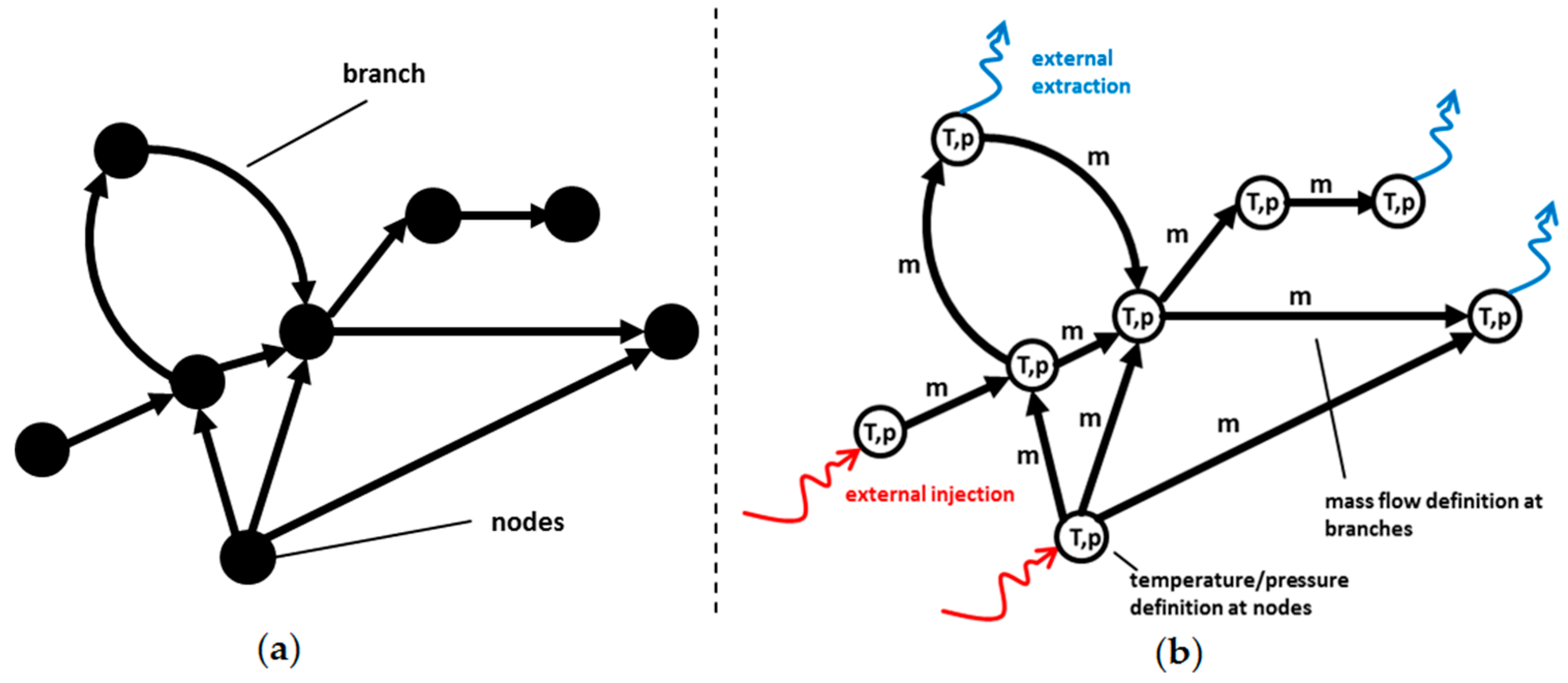Considering Figure 1a, a general graph network consists of $n$ nodes connected by $b$ branches.

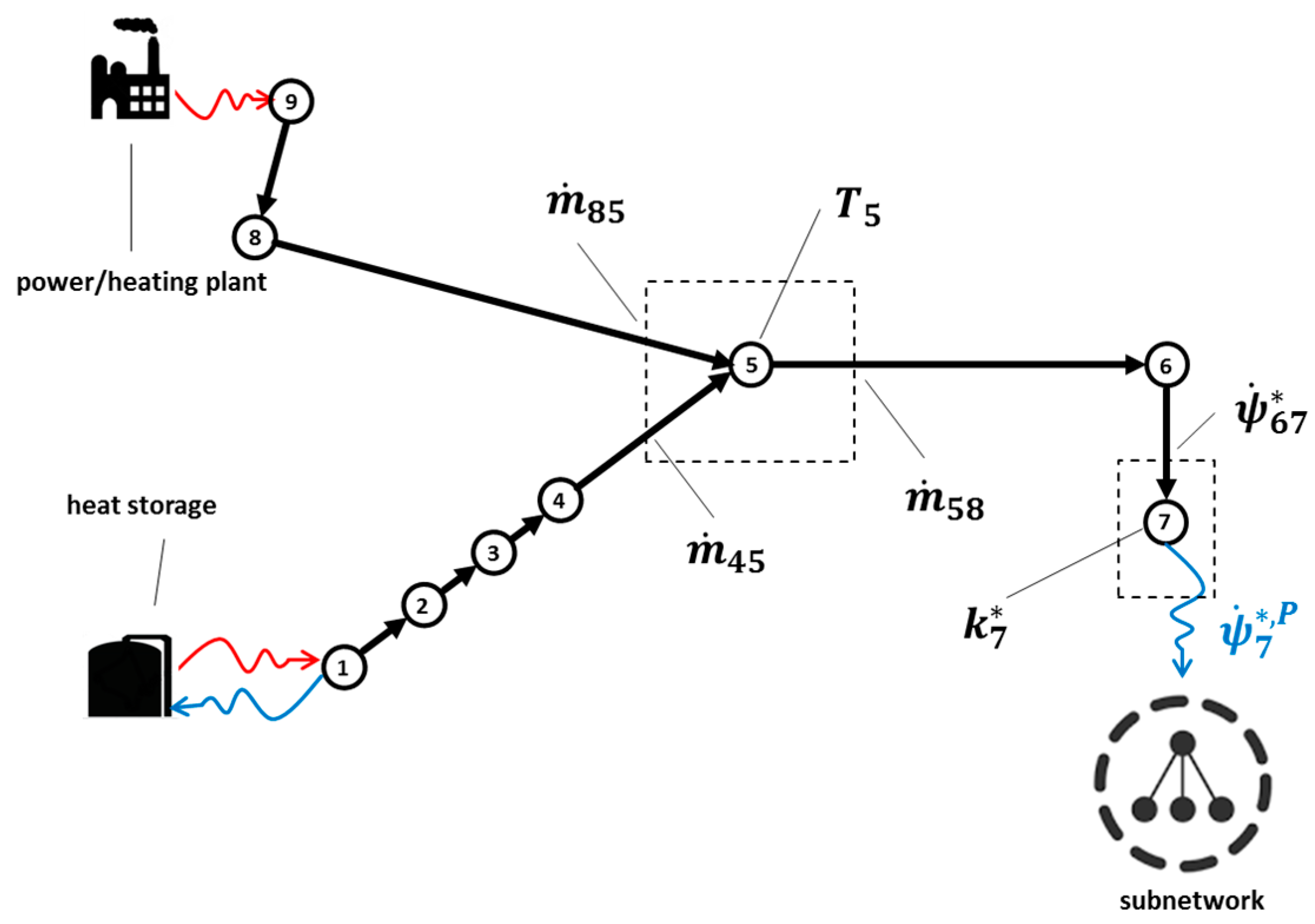
In thermal networks, the branches represent the pipes, while the nodes represent junctions/splitters where different pipes are connected. Despite the fact that heating networks are closed networks, usually they are represented as open networks, considering only the supply network. In this case, the boundary nodes are representing the thermal energy users or producers, i.e., the buildings connected with the network and the thermal plants. Based on that, mass flow rates are assigned to the branches, while temperatures and pressures are assigned to the network nodes. In nodes representing the users/producers, a mass flow rate is extracted/injected. Each branch is conventionally oriented. Inlet and outlet nodes can be identified according with their conventional verse. A mass flow rate is positive or negative depending if its real direction is coherent or opposite to the conventional one.

The result of that approach is a graph representation of the thermal network considering mass flows, temperature and pressure values as shown in Figure 1b.

According to graph theory [18], the topology of the graph, including the information of the connections between the nodes, can be described through the incidence matrix. The incidence matrix $\mathbf{A}\left(n\times b\right)$ provides information on the interconnections of the network. The general term $A_{ij}$ is equal to 1 if the i-th node is the inlet node of the j-th branch, while it is −1 if the node is the exiting node and it is 0 if the node is not related with the branch.

Different models to calculate mass flows, temperature and pressure values can be considered in a network. Nevertheless, this work focuses on the results that can be obtained by a thermo-fluid dynamic approach developed in [14], which is particularly suitable to effectively model transient operations in large networks with multiple loops. It must be noted that, in transient operation, both the thermodynamic properties and the directions of the hot water flow can change in time, which implies the calculation of time-dependent network properties.

2.2. Control Volume Definition and Exergetic Analysis

The exergetic analysis of the network provides the basis for the exergy cost approach and must be carried out using the results of the network model. As described before, the model result provides information about the mass flow rates of each branch and the temperature/pressure level at each node of the network. The control volume is essential for assigning exergy flows to branches and nodes of the network. 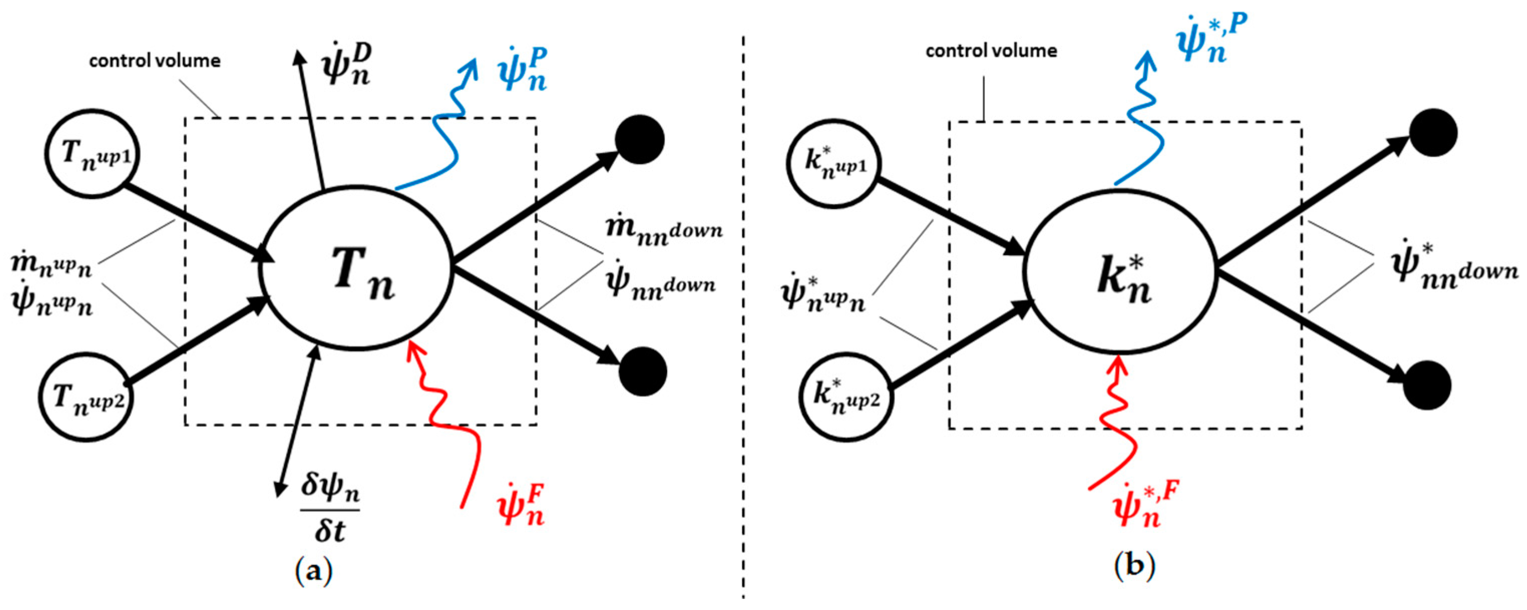Figure 2 shows the control volumes for both exergy and exergy cost analysis defined in this work.

The control volume defines the position of the exergy balance around the node and is shown in its general form in Figure 2a. Considering a generic node $n$, a distinction between upstream nodes $n^{up}$ and downstream nodes $n^{down}$ must be made according to the direction of the mass flow rates at a specific time-step. Upstream nodes are those supplying exergy to the control volume through entering mass flow rates, while downstream nodes extract exergy flow from the control volume through exiting mass flow rates.

In order to define the exergy flow crossing the control volume boundary, a numerical “upwind scheme” is applied. This is the same numerical scheme that is adopted for calculating temperature distributions in the network [14], while here it is extended to the exergetic costs. In general, the exergetic flow at the control volume boundary ${\dot{\psi }}_{n^{up}n}$ between node $n$ and its upstream node $n^{up}$ is a function of the mass flow rate ${\dot{m}}_{n^{up}n}$ in the branch crossing the control volume and the temperature and pressure of the upstream node $T_{n^{up}}$ and $p_{n^{up}}$ respectively.

The functional relation to evaluate the exergy flow exchanged at the control surface with surrounding control volumes is the definition of thermal and mechanical exergy according to [19]. In the case of entering flows, the expression for incompressible fluid is given in Equation (1)

$${\dot{\psi }}_{n^{up}n}={\dot{m}}_{n^{up}n}·\left\{c_p\left[T_{n^{up}}-T_0-T_0 ln\left(\frac{T_{n^{up}}}{T_0}\right)\right]+\frac{p_{n^{up}}-p_0}{\rho }\right\},$$

(1)

where $c_p$ is the specific heat, $T_0$ and $p_0$ are the ambient temperature and pressure values and $\rho$ is the fluid density.

In the case of exiting flows, node $n$ becomes the upstream node. Therefore, the properties of node $n$ should be considered for evaluating the exergy flows.

Exergy can be directly extracted from the node and supplied to an external user ${\dot{\psi }}_n^P$ or supplied to the node from an external producer ${\dot{\psi }}_n^F$. These streams are directly associated with the mass flow rates extracted or injected in the node, as indicated in Figure 1b. Equation (1) is used for their evaluation, where temperature and pressure are the source values in the case of entering flows and the node values in the case of exiting flows.

Furthermore, a transient term of exergetic flow must be considered to account for the time-dependent thermodynamic behavior of the network. It was already mentioned that directions of mass flow in the branches may change in time. In a steady-state condition, the temperature of the upstream node of a given branch always has a higher temperature than its downstream node, due to thermal losses. In case a change in direction takes place in a certain branch, the downstream node results in a higher temperature than its upstream node, which is followed by the effect that the downstream node cools down to a certain level lower than its upstream temperature. During that time, the exergy flow exiting the control volume of the downstream node is higher than the entering exergy flow, which would not be possible if only steady-state balance equations would be considered. During this cool-down phase, the downstream node is therefore providing previously-stored exergy to the control volume balance. Comprehensively, the same effect applies when node temperature increase, where also in this case, a transient term must be considered in order to avoid overestimation of exergy destruction. To account for this transient behavior, the change in exergy of the mass in the control volume $\frac{\delta {\psi }_n}{\delta t}$ of node $n$ must be considered and evaluated according to Equation (2)

$$\frac{\delta {\psi }_n}{\delta t}=M_n{c}_p\frac{\delta }{\delta t}\left[T_n-T_0-T_0 ln\left(\frac{T_n}{T_0}\right)\right],$$

(2)

where $M_n$ is the mass in the control volume of node $n$. For each branch, half of its mass is contributing to the control volume, except for nodes that have only one branch connected (such as user nodes). This is due to the energy balance formulation in the underlying thermo-fluid dynamic model. $M_n$ is then the sum of the contributions of all branches in the control volume $b_n^{con}$, while each contributing mass is calculated based on the geometric properties of the corresponding branch, length $l$ and diameter $d$ as well as fluid density $\rho$, see Equation (3):

$$\begin{gathered} M_n=\frac{\rho }{x}{{\displaystyle \sum }}_{b_n^{con}}{\left(\frac{d_{b_n^{con}}}{2}\right)}^2·\pi ·l_{b_n^{con}},\mathrm{with} \\ x=1 \text{for user nodes}, x=2 \text{for all other nodes} \end{gathered}$$

(3)

Simply speaking, the mass in the control volume, which must be evaluated to account for transient change in exergy, is the sum of half of the mass in each branch, except for user nodes.

No mechanical exergy is considered in Equation (2) since the fluid flow problem is typically written in steady state due to the much higher propagation velocity of pressure waves, which travel the network at the speed of sound, different to the advective flows, which travel the network at the fluid velocity.

The transient term $\frac{\delta {\psi }_n}{\delta t}$ can either be included negative or positive in the exergy balance. According to the formulation in Equation (2), the term $\frac{\delta {\psi }_n}{\delta t}$ is negative if node $n$ cools down, which implies that the absolute value of $\frac{\delta {\psi }_n}{\delta t}$ must be added as a fuel exergy stream to the control volume and vice versa.

Finally, a certain amount of exergy destruction at each node ${\dot{\psi }}_n^D$ must be considered due to irreversibilities in the network. Based on those terms, the exergy balance equation can be written down for node $n$ according to Equation (4)

$${\displaystyle \sum }_{n^{up}}{\dot{\psi }}_{n^{up}n}+{\dot{\psi }}_n^F-\frac{\delta {\psi }_n}{\delta t}-{\displaystyle \sum }_{n^{down}}{\dot{\psi }}_{n{n}^{down}}-{\dot{\psi }}_n^P-{\dot{\psi }}_n^D=0$$

(4)

Through applying the exergy balance of Equation (4), it is possible to calculate the amount of exergy destroyed in the control volume of each node in the network. The destruction of exergy is the major driving factor for increased exergetic costs at the network nodes, which is developed in the next subsection.

2.3. Exergetic Cost Balance

Exergetic cost ${\dot{\psi }}^{*}$ is a conservative value accounting for the amount of external exergy that is necessary to make an exergy flow available within a specific productive process [16]. A unit exergy cost $k^{*}$ can be defined by dividing the exergetic cost by the corresponding exergy, as in Equation (5)

$$k^{*}=\frac{{\dot{\psi }}^{*}}{\dot{\psi }},$$

(5)

assuming the primary resources with a unit exergy cost equal to one, unit exergy costs $k^{*}$ are thus a measure of the amount of irreversibilities, thus exergy destructions, which occur during the upstream processes in order to form a given exergy stream. Therefore, the higher the exergy destruction, the higher the unit exergy cost.

The definition of exergetic costs in Equation (5) is applied to the control volume in Figure 2a, leading to the exergetic cost balance for each node. As for exergy, exergetic costs are also defined at the border of the control volumes. The result can be seen in Figure 2b, which shows an example of a generic node having two entering exergy cost streams from upstream nodes ${\dot{\psi }}_{n^{up1}n}^{*}$ and ${\dot{\psi }}_{n^{up2}n}^{*}$ (resource flows), two exiting exergy cost streams ${\dot{\psi }}_{n{n}^{down1}}^{*}$ and ${\dot{\psi }}_{n{n}^{down2}}^{*}$ (product flows), one external exergy cost stream ${\dot{\psi }}_n^{*,F}$ (resource flow) entering, e.g., an exergy cost stream from an energy supplying unit and one external product exergy cost stream ${\dot{\psi }}_n^{*,P}$ (product flow), supplying, for instance, a connected subnetwork or consumer. This formulation of resources and products is not strictly necessary for calculation of costs but has been indicated in order to better relate the general nodal behavior with the prepositions proposed in the “theory of exergy cost”. Firstly, this definition does not contradict alternative formulations of resources and products in the case of mixing between different streams, as it occurs in the junctions. For example in the SPECO approach, the resource would be defined as the exergy decrease of the hotter stream and the product would be defined as the exergy increase of the colder stream [20]. In fact, in the present formulation, the exergetic cost of the node results through application of the exergy cost balance of the node. Secondly, the definition of the control volume, thus assigning a unit exergetic cost to each single node, assures that the principles of exergetic costing, are included: (1) the exergetic cost balance for a generic node $n$ is written as in Equation (6):

$${{\displaystyle \sum }}_{n^{up}}{\dot{\psi }}_{n^{up}n}^{*}+{\dot{\psi }}_n^{*,F}-k_n^{*}\left[{\dot{\psi }}_n^P+{{\displaystyle \sum }}_{n^{down}}{\dot{\psi }}_{n{n}^{down}}\right]=0,$$

(6)

(2) multi-product flows have equal unit exergetic costs, which is the unit cost of the node through the upwind scheme; (3) unit costs of exergy streams entering the system from outside, i.e., from the external producers, are imposed through Dirichelet boundary conditions, in agreement with the thermal model. This means that costs are calculated without any specific application of the prepositions, but only proceeding coherently with the numerical scheme adopted for solving the energy equation.

The cost balance at node $n$ evaluates the unit exergy costs $k_n^{*}$ based on the cost flows entering and exiting the control volume. This approach can be applied to each node in the network leading to a set of linear systems that can be numerically solved. In order to provide a compact formulation for graph-based networks, a matrix formulation is developed which uses the network topology and its characteristic properties only.

2.4. Matrix Formulation of the Approach

In this section, the matrix formulation for the exergetic cost balance is developed. The aim is to provide an analytical matrix formulation on the basis of the network topology. To represent the network topology, the incidence matrix $\mathit{A}$ is used:

$$\begin{gathered} \mathit{A}=\left[\begin{array}{ccc}{a}_{1,1}& \cdots & a_{1,b}\\ ⋮& \ddots & ⋮\\ a_{n,1}& \cdots & a_{n,b}\end{array}\right],\mathrm{with} \\ {a}_{n,b}=-1 \text{for the branches b entering node n}, \\ {a}_{n,b}=+1 \text{for the branches b exiting node n}. \end{gathered}$$

(7)

It is worth mentioning, that to apply the upwind scheme, the real verses of mass flow rates should be considered instead of the conventional ones. This means that the incidence matrix should be updated at each time step of the analysis once the fluid flow problem is solved, by changing the signs in each column corresponding with negative mass flow rates.

Furthermore, the exergy flows exchanged between all control volumes of the network, i.e., the flows in all branches, can be casted in an exergy flow vector $\dot{\mathit{\psi }}$ $\left(b\times 1\right)$. Another vector ${\dot{\mathit{\psi }}}_{\mathit{trans}}$ $\left(n\times 1\right)$ is needed to include information on the amount of exergy stored/released in each control volume based on its transient behavior. The boundary conditions associated with the external fuel costs are imposed in the vector ${\mathit{\psi }}^{*,\mathit{F}}$ $\left(n\times 1\right)$, while the costs of extracted flows appear in vector ${\mathit{\psi }}^{\mathit{P}}$ $\left(n\times 1\right)$. Equations (8)–(11) show the defined vectors:

$$\dot{\mathit{\psi }}=\left[\begin{array}{c}{\dot{\psi }}_1\\ {\dot{\psi }}_2\\ \dots \\ {\dot{\psi }}_b\end{array}\right]$$

(8)

$${\dot{\mathit{\psi }}}_{\mathit{trans}}=\frac{1}{\delta t}\left[\begin{array}{c}\delta {\psi }_1\\ \delta {\psi }_2\\ \dots \\ \delta {\psi }_n\end{array}\right]$$

(9)

$${\dot{\mathit{\psi }}}^{\mathit{P}}=\left[\begin{array}{c}{\dot{\psi }}_1^P\\ {\dot{\psi }}_2^P\\ \dots \\ {\dot{\psi }}_n^P\end{array}\right]$$

(10)

$${\dot{\mathit{\psi }}}^{*,\mathit{F}}=\left[\begin{array}{c}{\dot{\psi }}_1^{*,F}\\ {\dot{\psi }}_2^{*,F}\\ \dots \\ {\dot{\psi }}_n^{*,F}\end{array}\right]$$

(11)

Through the use of matrix representation of Equations (7)–(11), the exergetic cost balance in Equation (6) can be rewritten as in Equation (12):

$$\left\{\left[\mathit{A}\times \mathit{I}\dot{\mathit{\psi }}\times {\left[{\mathit{A}}^{+}\right]}^{\mathit{T}}\right]+\mathit{I}\left[{\dot{\mathit{\psi }}}^{\mathit{P}}-{\dot{\mathit{\psi }}}_{\mathit{trans}}\right]\right\}{\mathit{k}}^{*}={\dot{\mathit{\psi }}}^{*,\mathit{F}},$$

(12)

where $\mathit{I}$ is the identity matrix and matrix ${\mathit{A}}^{+}$ $\left(n\times b\right)$ is the positive part of the incidence matrix and can be obtained through applying Equation (13) to each matrix entry:

$$a_{n,b}^{+}=max\left(a_{n,b},0\right)$$

(13)

This approach can be used for any type of DHN topology, where every branch is connected with two nodes. The result is the calculation of unit exergetic costs at network nodes ${\mathit{k}}^{*}$, which provides information on thermodynamic-based costs of exergy destruction at network nodes. Based on Equation (12), ${\mathit{k}}^{*}$ is evaluated numerically for a specific time-step. When analyzing the time-dependent behavior of the thermal network, Equation (12) must be applied to each single time-step. In that case, each term must be evaluated based on current exergy flows and the actual directions in the branches. Therefore, both $\mathit{A}$ and the exergy-based vectors of Equations (8)–(11) must be updated according to the actual condition. For a given timeframe $\mathit{t}$, a time-dependent unit exergy cost matrix ${\mathit{K}}^{*}$ $\left(n\times t\right)$ can be derived, which shows the unit exergy cost behavior of each node in time.

This approach is especially suitable for application to large networks because its formulation is based on the network topology and can therefore be easily integrated into the numerical algorithm, which is coherent with the one used for calculating temperature and pressure evolutions. Furthermore, information on external exergy costs is integrated into ${\dot{\mathit{\psi }}}^{*,\mathit{F}}$, which makes additional auxiliary equations unnecessary. This avoids increasing the problem size and reduces computation costs compared to the classical formulation, while the principles of exergetic costing are integrated. It must be noted that, in the case of real applications, economic costs like capital, operating and maintenance costs must also be considered as external exergy cost flows. Based on the provided matrix formulation in Equation (12), those costs can comfortably be included in ${\dot{\mathit{\psi }}}^{*,\mathit{F}}$.

3. Case Study: Example Thermal Heat Network

In this section, the proposed thermoeconomic formulation is applied to an example of a thermal network which consists of nine nodes connected via eight branches as can be seen in Figure 3. This is a small portion of the DHN in Turin located in Italy, where a power/heating plant and a thermal heat storage are connected. This network is chosen in order to show the exergetic cost behavior in a transient operating condition, which is derived from a time-dependent supply of heat by the power plant and the storage unit.

The case-study data is taken from previous projects, previously analyzed in [14], which have analyzed the thermo-fluidynamic behavior of the network. The lengths of the branches shown in Figure 3 are proportional to their real lengths in the network. Based on the data available, the heating plant is supplying the network with hot water at a constant temperature of 120 °C and a mass flow rate depending on the thermal request of the consumer, which, in this example, corresponds to the subnetwork in Figure 3. The thermal request is modeled as a mass flow rate extracted from node 7. Correspondingly, an exergy flow is extracted from node 7 ${\dot{\psi }}_7^P$ and supplied to the rest of the network (not represented here). The storage unit is connected to node 1 and can be operated either in charging or discharging mode, thus either extracting or injecting exergy to the network.

The aim of the analysis is to derive the unit exergy cost of heat in the network and particularly in node 7 $k_7^{*}$, which represents the costs of heat supplied to the network. If, e.g., an external consumer were connected to that node, a unit exergy costs could be assigned to the final use of that exergy stream.

Considering the example network, the heating plant is supplying mass flow at a certain temperature level into the network, while the storage is either supplying or extracting mass flow of the network. Therefore, each branch has a certain mass flow while, for each node, a temperature is assigned. Based on the results provided by the thermo-fluidynamic model, the network properties can be calculated and are exemplarily shown for the control volume of node 5 in Figure 4.

The figure shows both mass flow rates and temperature evolution for a timeframe between 20:00 $\left(t=0\right)$ and 11:00 $\left(t=900\right)$ for a typical day throughout the heating season in Turin. The mass flow coming from the path of the heating plant ${\dot{m}}_{85}$ varies between 500 and 1300 kg/s with a peak during the morning hours at about $t=670$. The mass flow corresponding to the injection or extraction from the storage ${\dot{m}}_{45}$ shows a low supply at the beginning followed by a stand-by and a charging phase during the nighttime ($180<t<600$). The charging is represented through negative mass flow values of ${\dot{m}}_{45}$. During the stand-by, the model assumes a very small mass flow in order to avoid numerical issues. Temperatures in the branches connecting the storage unit to the remaining part of the network register a drop because, in this operating regime, heat losses do not change significantly, while the heat transferred becomes almost zero. In the quasi-steady state conditions, temperature decreases along the flow direction, e.g., at $0<t<80$, $T_8>T_5>T_6$.

This might not be the case during transient conditions, where the directions of the mass flow change and, therefore, a downstream node shows a higher temperature level than its upstream node. Due to the fact that the storage mode changes from charging to discharging and vice versa, the temperature levels along the path of the storage are highly affected by the changing supply of different mass flows at different temperatures.

4. Results and Discussion

The result of exergetic cost analysis is given in Figure 5, showing the relative increase of normalized unit exergy costs of the nodes $\Delta k_n^{norm}$ for two different network conditions. The relative normalized unit exergy costs $\Delta k_n^{*,norm}$ are derived through Equation (14)

$$\Delta k_n^{*,norm}=k_n^{*}-k_{supply}^{*},$$

(14)

where $k_{supply}^{*}$ is the unit exergy cost of the external flow at the plant and storage nodes. This representation is used in order to show the evolution of $k_n^{*}$ throughout the network, regardless of the unit exergy costs of external inflows. In this case, $k_{supply}^{*}=1$ is assumed for the thermal plant. This value needs to be calculated from exergy cost analysis applied to the thermal production from fossil fuel in order to account for the irreversibilities occurring in the cogeneration system.

A quasi-steady state condition is presented at $t=50$, while the transient condition is shown at $t=193$, corresponding to the behavior of mass flow and temperature of Figure 4. In the examined pseudo steady state condition, the storage system is not operating. As discussed above, a fictitious supply characterized by a very small mass flow rate at the ambient temperature is assumed as the boundary condition; therefore, the exergy associated with this stream is zero. A unit exergy cost $k_{supply}^{*}=1$ is considered for the storage node during stand-by. In this condition, unit exergy costs increase from node 1 to node 4 as well as from node 9 to node 8 because of the irreversibilities associated with heat losses. Unit exergy cost in node 5 is considerably lower than in node 4, due to the fact that almost no exergy is supplied from that part of the network because of the very small fluid flow at the current temperature level of the control volumes 1–4. Cost of exergy in node 5 is thus mainly due to the cost increase between nodes 9, 8 and 5. For nodes 6 and 7, unit costs further increase due to exergetic losses.

During the transient phase, the storage is operated in charging mode, extracting exergy from the network at given unit costs. This leads to a change in direction for the branches between node 5 and 1, while only node 9 is left supplying exergy to the network. In this case, unit exergy costs increase from node 9 to node 5 as well as from node 5 to node 1 and to node 7. Again, it can be seen that the increase of unit costs is higher at the storage path, where $\Delta k_1^{*,norm}$ is much larger than $\Delta k_7^{*,norm}$. This means that the unit exergy cost of exergy extracted at the storage node is considerably higher than the exergy extracted at the subnetwork; in fact, no significant changes in the unit exergy costs between quasi-steady state and transient conditions take place in nodes 5–9.

Furthermore, the transient condition leads to a higher unit exergy increase in the transient than in the quasi-state condition in the storage path. This cost is about 1% of the unit cost of thermal exergy supplied by the plant to the district heating network, which means that this term cannot be neglected in the analysis.

The unit exergy cost of storage during the discharge phase is set based on a time-evolution of costs during the charging phase. During discharge, a constant unit cost equal to the average cost registered during charging phase is considered. Theoretically, the irreversibilities associated with stand-by, i.e., the heat losses of the storage tank and thermal de-stratification inside the tank should be considered, but here these have been neglected.

The last part covers the analyses of the evolution of unit exergy costs for network nodes in time. Since node 7 is the connection to the subnetwork, its unit exergy cost evolution is highly interesting since it determines the costs at which the rest of the network is supplied by exergy coming from the supplying units. Again, the relative representation through $\Delta k_7^{*,norm}$ is used to explicitly show the network behavior in Figure 6.

It can be seen that $\Delta k_7^{*,norm}$ increases during the timeframe $80<t<180$, which corresponds to the time, where the storage mode changes from stand-by to charging. During that phase, mass flow at the storage path changes its direction and temperature in the control volumes 1–4 increases (see Figure 4), which affects the unit exergy cost formation of the whole network. During the discharging and charging phases, unit exergy costs remain mainly constant, while during the transition time, when the storage mode changes, unit exergy costs are increased. This is another indication for an increased unit exergy cost during high changes of temperature levels at the network nodes caused by the actual exergy flow through the network.

The unit exergy cost is an important techno-economic indicator, which can be used to estimate the economic “burden” of providing heating as an energy service to a specific costumer. Thus, it helps in defining the potential of demand side measures, e.g., heat load optimization, where the impact of such measures will be higher for consumers showing higher exergetic costs. Furthermore, prediction of the exergetic costs of future consumers, depending on their load profile and position in the network, can be carried out.

5. Conclusions

In this work, a new approach for effective application of exergy cost analysis to graph-based network models was developed. The approach is consistent with the principles of exergetic costing while it is suitable for large thermal networks avoiding the use of auxiliary equations in order not to increase the problem dimension. This is crucial in the case where large networks are examined. The approach is based on an upwind scheme formulation in which applications to (very) large network sizes are theoretically possible, limited only by the numerical resolution (control volumes) and/or the computational effort.

Based on a previously deployed transient thermal network model, exergy and exergy cost balances were defined for control volumes of network nodes. This enabled direct use of the network topology and its characteristic properties considering time dependent operation. The method allows for one investigating the formation of unit exergy costs of any subgraph in the network with which more information, on where and when unit exergy costs increase, can be extracted. This is an important piece of information that can profitably be of use for improving or optimizing district heating network design and operation.

The approach was applied to an example network, which provides detailed insights into exergy cost formation during transient system condition. Results show that the costs related with transient operation are not negligible. Especially when it comes to large networks including daily storage and volatile predictable (waste heat) or unpredictable (renewables) energy sources, this formulation is able to analyse its exergetic effects on the network behavior.

The proposed approach is thus suitable for thermoeconomic analysis of district heating networks; especially in the case when their operation involves time variations in supply/return temperatures, the use of intermittent energy (exergy) sources or storage. This provides the basis for the assessment of the integration of storage and temperature-dependent energy sources that are appreciated by the development of 4th generation district heating networks.

References

1. Tribus, M.; Evans, R.B. A Contribution to the Theory of Thermoeconomics; UCLA Report No. 6236; University of California: Los Angeles, CA, USA, August 1962. [Google Scholar]
2. Tsatsaronis, G.; Pisa, J. Exergoeconomic Evaluation and Optimization of Energy Systems—The CGAM Problem. Energy 1994, 19, 287–321. [Google Scholar] [CrossRef]
3. El Sayed, Y.M. The Thermoeconomics of Energy Conversions; Elsevier: Amsterdam, The Netherlands, 2003. [Google Scholar]
4. Torres, C.; Valero, A.; Serra, L.; Royo, J. Structural theory and thermoeconomic diagnosis: Part I. On malfunction and dysfunction analysis. Energy Convers. Manag. 2002, 43, 1503–1518. [Google Scholar] [CrossRef]
5. Verda, V.; Baccino, G. Thermoeconomic approach for the analysis of control system of energy plants. Energy 2012, 41, 38–47. [Google Scholar] [CrossRef]
6. Baldvinsson, I.; Nakata, T. A comparative exergy and exergoeconomic analysis of a residential heat supply system paradigm of Japan and local source based district heating system using SPECO (specific exergy cost) method. Energy 2014, 74, 537–554. [Google Scholar] [CrossRef]
7. Baldvinsson, I.; Nakata, T. A feasibility and performance assessment of a low temperature district heating system—A North Japanese case study. Energy 2016, 95, 155–174. [Google Scholar] [CrossRef]
8. Gładysz, P.; Ziebik, A. Complex analysis of the optimal coefficient of the share of cogeneration in district heating systems. Energy 2013, 62, 12–22. [Google Scholar] [CrossRef]
9. Keebaş, A.; Ali Alkan, M.; Bayhan, M. Thermo-economic analysis of pipe insulation for district heating piping systems. Appl. Therm. Eng. 2011, 31, 3929–3937. [Google Scholar] [CrossRef]
10. Keçebaş, A. Performance and thermo-economic assessments of geothermal district heating system: A case study in Afyon, Turkey. Renew. Energy 2011, 36, 77–83. [Google Scholar] [CrossRef]
11. Verda, V.; Kona, A. Thermoeconomics as a tool for the design and analysis of energy savings initiatives in buildings connected to district heating networks. Int. J. Thermodyn. 2012, 15, 221–229. [Google Scholar] [CrossRef]
12. Verda, V.; Caccin, M.; Kona, A. Thermoeconomic cost assessment in future district heating networks. Energy 2016, 117, 485–491. [Google Scholar] [CrossRef]
13. Verda, V.; Guelpa, E.; Kona, A.; Lo Russo, S. Reduction of primary energy needs in urban areas trough optimal planning of district heating and heat pump installations. Energy 2012, 48, 40–46. [Google Scholar] [CrossRef]
14. Guelpa, E.; Toro, C.; Sciacovelli, A.; Melli, R.; Sciubba, E.; Verda, V. Optimal operation of large district heating networks through fast fluid-dynamic simulation. Energy 2016, 102, 586–595. [Google Scholar] [CrossRef]
15. Li, H.; Svendsen, S. Energy and exergy analysis of low temperature district heating network. Energy 2012, 45, 237–246. [Google Scholar] [CrossRef]
16. Lozano, M.A.; Valero, A. Theory of exergetic cost. Energy 1993, 18, 939–960. [Google Scholar] [CrossRef]
17. Sciacovelli, A.; Verda, V.; Borchiellini, R. Numerical Design of Thermal Systems; CLUT: Torino, Italy, 2013. [Google Scholar]
18. Zawislak, S.; Rysinski, J. Graph-Based Modelling in Engineering; Springer: Berlin/Heidelberg, Germany, 2016. [Google Scholar]
19. Kotas, T.J. The Exergy Method of Thermal Plant Analysis; Krieger Publishing: Malabar, FL, USA, 1995. [Google Scholar]
20. Lazzaretto, A.; Tsatsaronis, G. SPECO: A systematic and general methodology for calculating efficiencies and costs in thermal systems. Energy 2006, 31, 1257–1289. [Google Scholar] [CrossRef]
Figure 1. (a) Simple directed graph; (b) thermal graph network.
Entropy 19 00109 g001
Figure 2. Control volumes for (a) exergy and (b) exergy cost analysis.
Entropy 19 00109 g002
Figure 3. Example of thermal network.
Entropy 19 00109 g003
Figure 4. Mass flows and temperature levels for node 5.
Entropy 19 00109 g004
Figure 5. Δ k n * , n o r m -values for a network in quasi-steady state and transient condition.
Entropy 19 00109 g005
Figure 6. Unit exergy cost evolution of node 7.
Entropy 19 00109 g006