The Two-Time Interpretation and Macroscopic Time-Reversibility

Abstract

The two-state vector formalism motivates a time-symmetric interpretation of quantum mechanics that entails a resolution of the measurement problem. We revisit a post-selection-assisted collapse model previously suggested by us, claiming that unlike the thermodynamic arrow of time, it can lead to reversible dynamics at the macroscopic level. In addition, the proposed scheme enables us to characterize the classical-quantum boundary. We discuss the limitations of this approach and its broad implications for other areas of physics.

1. Introduction

Meeting the infamous measurement problem of quantum mechanics is the primary aim of its various interpretations. The measurement problem arises from the clash between the two evolution laws of quantum theory: the deterministic Schrödinger equation which is obeyed by isolated microscopic systems, and the non-deterministic (probabilistic) “collapse” into a specific eigenstate of the measured observable, which occurs upon encounter with the macroscopic world through the act of measurement. The idea that physical domains are demarcated by the process of measurement is far too anthropic. It is unacceptable for a fundamental physical theory to regard measurements as a primitive irreducible process. However, if measurements are reducible to a mere large-scale quantum interaction between a multi-particle macro-system on the one hand, and a few-particles micro-system on the other hand, then they should be within the scope of the Schrödinger equation, in which case determinism would have been ubiquitous, in conflict with collapse. Thus by rejecting the irreducibility of measurement, we render the two evolution laws incompatible. Hence, the problem.

It is generally understood that a measurement involves an amplification of a microscopic superposition into the macroscopic realm by means of entanglement, followed by decoherence by the environment [1,2]. However, without collapse one is left with a superposition of worlds where a different outcome occurs in each. From the perspective of a single “world” (or branch), the system is a mixture of effectively classical states; globally, however, the system is still macroscopically superposed. Read literally, this is the many-morlds interpretation (MWI) due to Everett.

In classical mechanics, initial conditions specifying the position and velocity of every particle and the forces acting on them fully determine the time evolution of the system. Therefore, trying to impose a final condition would either lead to redundancy or inconsistency with the initial conditions. However, in quantum mechanics, adding any non-orthogonal final condition is consistent. We contend that the addition of a final (backward-evolving) state-vector results in a more complete description of the quantum system in between these two boundary conditions. The utility of the backward-evolving state-vector was demonstrated in the works of Aharonov et al., but here we shall claim that this addition goes beyond utility. We propose a mechanism based on the two-state vector-formalism (TSVF) [3,4,5,6,7,8,9,10,11], where in each measurement a single outcome is chosen by a second quantum state evolving backwards in time. Generalizing this to the entire Universe, we develop an interpretation where the initial and final states of the Universe together determine the results of all measurements. This has the virtue of singling out just one “world”. We thus propose an answer to the question that (to our view) best encapsulates the measurement problem—how does a measurement of a superposed state give rise to an experience of a single outcome? It does so by means of a second state vector propagating from the future to the past and selecting a specific outcome.

In this framework, the emergence of specific macrostates seems non-unitary from a local perspective, and constitutes an effective “collapse”—a term which will be used here to denote macroscopic amplification of microscopic events—complemented by a reduction via the final state. We will show that a specific final state can be assigned so as to enable macroscopic time-reversal or “classical robustness under time-reversal”; that is, reconstruction of macroscopic events in a single branch, even though “collapses” have occurred. An essential ingredient in understanding the quantum-to-classical transition is the robustness of the macrostates comprising the measuring apparatus, which serves to amplify the microstate of the measured system and communicate it to the observer. The robustness guarantees that the result of the measurement is insensitive to further interactions with the environment. Indeed, microscopic time-reversal within a single branch is an impossible task because evolution was effectively non-unitary. Macroscopic time-reversal—which is the one related to our every-day experience—is possible, although non-trivial.

2. The Two-States-Vector Formalism

The basis for a time-symmetric formulation of quantum mechanics was laid in 1964 by Aharonov, Bergman, and Lebowitz (ABL), who derived a probability rule concerning measurements performed on systems, with a final state specified in addition to the usual initial state [3]. Such a final state may arise due to a post-selection; that is, performing an additional measurement at some late time on the system and considering only the cases with the desired outcome (here we assume for deductive purposes that a measurement generates an outcome, postponing the explanation to the next section). Given an initial state $|\mathsf{\Psi }\rangle$ and a final state $|\mathsf{\Phi }\rangle$ , the probability that an intermediate measurement of the non-degenerate operator $A={\sum }_k{a}_k{A}_k$ yields an eigenvalue $a_k$ is

$$\begin{array}{c}Pr\left(a_k|\mathsf{\Psi },\mathsf{\Phi }\right)=\frac{{\left|\langle \mathsf{\Phi }\left|A_k\right|\mathsf{\Psi }\rangle \right|}^2}{{\sum }_j{\left|\langle \mathsf{\Phi }\left|A_j\right|\mathsf{\Psi }\rangle \right|}^2}\hfill \end{array}$$

(1)

For simplicity, no self-evolution of the states is considered between the measurements. If only an initial state is specified, Equation (1) should formally reduce to the regular probability rule:

$$Pr\left(a_k|\mathsf{\Psi }\right)={\left|〈a_k|\mathsf{\Psi }〉\right|}^2$$

(2)

This can be obtained by summing over a complete set of final states, expressing the indifference to the final state. However, we can also arrive at Equation (2) from another direction [7]. Notice that if the final state is one of the eigenstates, $|\mathsf{\Phi }\rangle =|a_k\rangle$, then Equation (1) gives probability 1 for measuring $a_k$, and probability 0 for measuring any orthogonal state. Consider now an ensemble of systems of which fractions of size ${\left|〈a_k|\mathsf{\Psi }〉\right|}^2$ happen to have the corresponding final states $a_k$. The regular probability rule (Equation 2) of quantum mechanics is then recovered, but now the probabilities are classical probabilities due to ignorance of the specific final states. The same would be the result for a corresponding final state of an auxiliary system (such as a measuring device or environment), correlated with the measured system. This reduction of the ABL rule to the regular probability rule is a clue, showing how a selection of appropriate final states can account for the empirical probabilities of quantum measurements [7].

This possibility of a final state to influence the measurement statistics has motivated the re-formulation of quantum mechanics (QM) as taking into account both initial and final boundary conditions. Within this framework, QM is time-symmetric. The Schrödinger equation is linear in the time derivative, and therefore only one temporal boundary condition may be consistently specified for the wavefunction. If both initial and final boundary conditions exist, we must have two wavefunctions—one for each. The first is the standard wavefunction (or state vector), evolving forward in time from the initial boundary condition. The second is a (possibly) different wavefunction evolving from the final boundary condition backwards in time. Thus, the new formalism is aptly named the TSVF. A measurement—including a post-selection—will later be shown to constitute an effective boundary condition for both wavefunctions. Accordingly, we postulate that the complete description of a closed system is given by the two-state:

$$\langle \mathsf{\Phi }\left|\right|\mathsf{\Psi }\rangle ,$$

(3)

where $|\mathsf{\Psi }\rangle$ and $\langle \mathsf{\Phi }|$ are the above initial and final states, which we term the forward and backward-evolving states (FES and BES), respectively. These may be combined into an operator form by defining the “two-state density operator”:

$$\rho \left(t\right)=\frac{\left|\mathsf{\Psi }\left(t\right)\right.〉\left.〈\mathsf{\Phi }\left(t\right)\right|}{〈\mathsf{\Psi }\left(t\right)|\mathsf{\Phi }\left(t\right)〉},$$

(4)

where orthogonal FES and BES at any time t are forbidden. For a given Hamiltonian $H\left(t\right)$, the two-state evolves from time $t_1$ to $t_2$ according to

$$\rho \left(t_2\right)=U(t_2,t_1)\rho \left(t_1\right)U(t_1,t_2),$$

(5)

where $U(t_2,t_1)$ is the regular evolution operator:

$$U(t_2,t_1)=Texp\left(-i\underset{t_1}{\overset{t_2}{\int }}H\left(\tau \right)d\tau /\hslash \right)$$

(6)

(T signifies the time ordered expansion). The reduced two-state describing a subsystem is obtained by tracing out the irrelevant degrees of freedom.

In standard QM, we may also use an operator form similar to the above, replacing the state vector $\mathsf{\Psi }\left(t\right)$ with the density matrix:

$$\rho \left(t\right)=\left|\mathsf{\Psi }\left(t\right)\right.〉\left.〈\mathsf{\Psi }\left(t\right)\right|$$

(7)

The density matrix again evolves by Equation (7), and once more the reduced density matrix for a subsystem is obtained by tracing out the irrelevant degrees of freedom. Excluding measurements, the density matrix is a complete description of a system, evolving unitarily from initial to final boundary. Such systems can be thought of as two-time systems having FES and BES that are equal at any time; i.e., with a trivial final boundary condition that is just the initial state evolved unitarily from the initial time $t_i$ to the final time $t_f$,

$$\left|{\mathsf{\Psi }}_f\right.〉=U\left(t_f,t_i\right)\left|{\mathsf{\Psi }}_i\right.〉$$

(8)

We take Equation (8) as a zero-order approximation of the final boundary condition. By considering final boundary conditions deviating from the above, we may introduce a richer state structure into the quantum theory. When would this special final boundary condition be shown to affect the dynamics? It would do so if the reduced two-state describes a subsystem for which the ignored degrees of freedom do not satisfy Equation (8). Then, the reduced two-state should replace the density matrix, which is no longer a reliable description of the state of the system.

3. The Two-Time Interpretation

The TSVF provides an extremely useful platform for analyzing experiments involving pre- and post-selected ensembles. Weak measurements enable us to explore the state of the system during intermediate times without causing an effective disturbance [12,13]. The power to explore the pre- and post-selected system by employing weak measurements—and the concomitant emergence of various novel phenomena—motivates a literal reading of the formalism; that is, as more than just a mathematical tool of analysis. It motivates a view according to which future and past play equal roles in determining the quantum state at intermediate times, and are hence equally real. Accordingly, in order to fully specify a system, one should consider two state vectors.

A measurement generally yields a new outcome state of the quantum system and the measuring device. This state may be treated as an effective boundary condition for both future and past events. We suggest that it is not the case that a new boundary condition is independently generated at each measurement event by some unclear mechanism. Rather, the final boundary condition of the Universe includes the appropriate final boundary conditions for the measuring devices which would evolve backward in time to select a specific measurement outcome. In the following sections we shall demonstrate how this boundary condition arises at the time of measurement due to a two-time decoherence effect. Indeed, we will see that in the pointer basis (determined by decoherence [1,2]), the outcome of the measurement can only be the single classical state corresponding to the final boundary condition. The upshot is that in this way we can see how measurements may have a definite outcome without resorting to collapse. Viewed this way, the unpredictability of the outcome is due solely to the inaccessibility of the BES. The forgoing amounts to a two-time interpretation (TTI) of quantum mechanics.

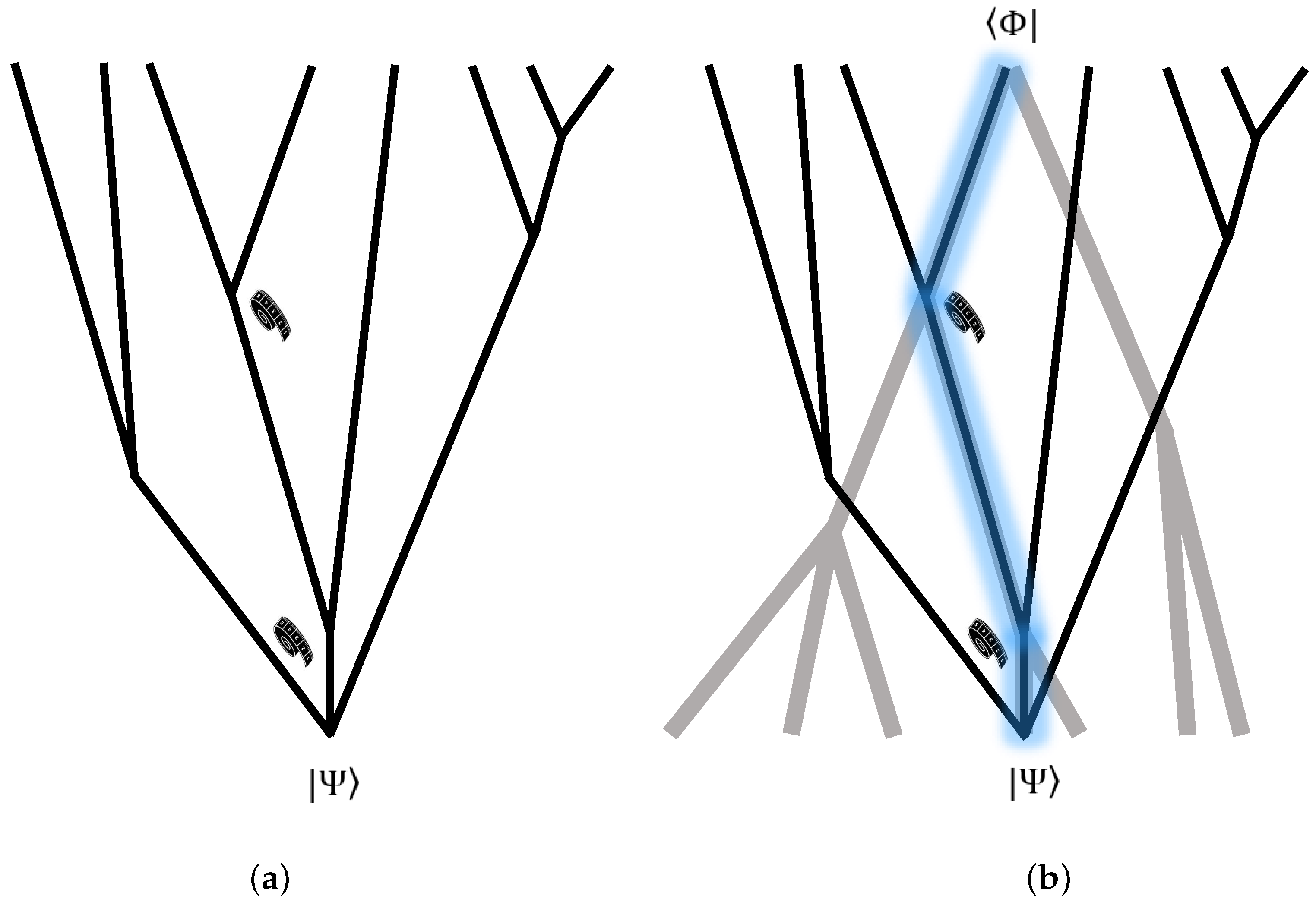
The TTI is an ontological interpretation of QM akin to the MWI which postulates two branching wavefunctions whose conjunction delineates a single history out of the MWI picture (see Figure 1).

Because the universal two-state at one time determines the universal two-state in all times, the interpretation is deterministic, with the caveat that it is nevertheless principally unpredictable. A similar case appears in Bohmian mechanics, which is generally regarded to uphold determinism. Indeed, like Bohmian mechanics, the TTI can be viewed as a hidden variable interpretation—in the sense that the BES is unknown and unknowable, and yet it completes the theory [9,10]. The probabilistic properties of QM are consequent upon the hidden nature of the BES. Accessibility of the BES leads to a violation of causality. To see this, consider the following example: two spin-1/2 particles are entangled in the state ${\left|\uparrow \right.〉}_A{\left|\uparrow \right.〉}_B+{\left|\downarrow \right.〉}_A{\left|\downarrow \right.〉}_B$, where A and B denote spatially separated Alice and Bob. Assume the opposite, that Bob knows the final state to be ${\left|\uparrow \right.〉}_A{\left|\uparrow \right.〉}_B+{\left|\uparrow \right.〉}_A{\left|\downarrow \right.〉}_B$. Now, Alice may or may not perform a unitary rotation on her particle, of the form ${\left|\uparrow \right.〉}_A\rightleftharpoons {\left|\downarrow \right.〉}_A$, leaving the initial composite state idle, or transforming it into the state ${\left|\downarrow \right.〉}_A{\left|\uparrow \right.〉}_B+{\left|\uparrow \right.〉}_A{\left|\downarrow \right.〉}_B$. For the case where Alice performs the transformation, the reduced density matrix of Bob’s particle is ${\rho }_B=\left|\downarrow \right.〉\left.〈\downarrow \right|$; for the case she does not, it is ${\rho }_B=\left|\uparrow \right.〉\left.〈\uparrow \right|$. Accordingly, if Bob measures the spin of his particle, he will obtain ${\left|\downarrow \right.〉}_B$ or ${\left|\uparrow \right.〉}_B$, depending on the action or non-action of Alice. In this manner, Alice may allegedly transmit signals to Bob at an instant [7], in violation of no-signaling.

Accordingly, while the TSVF is in principle a time symmetric approach, there are operational differences between the FES and BES. It is possible to prepare any FES by performing a measurement and then unitarily transform the resulting state to the desired state. However, because the outcome of a state-preparing measurement can be known only after it is performed, this strategy will not work for the BES.

Even though TSVF is analogous to a subtle local hidden variable theory [9,10] (unlike Bohmian mechanics, which is manifestly non-local), which Bell’s argument supposedly rules out, it is immune to the argument. The reason is that the BES contains outcomes only of measurements which are actually performed, precluding counterfactual measurements, which are necessary for Bell’s case. Viewed as a retrocausal model, the TSVF is thus understood to be nonlocal in space, but local in spacetime [9]. An additional requirement is that the final state in the pointer basis will induce—backwards in time— an appropriate distribution of outcomes so as to recover the empirical quantum mechanical probabilities for large ensembles, given by the Born rule. The determination of the measurement statistics by the correspondence between the two states may lead one to conclude that within the framework of TTI, the Born rule is contingent upon the boundary conditions. However, this is inaccurate. It can be shown that this specific law follows—in the infinite N limit—from the compatibility of quantum mechanics with classical-like properties of macroscopic objects [5,6]. Under the assumption that the results of physical experiments are stable against small perturbations for macroscopically large samples, a final state upholding the Born rule is the only one that is consistent with weak measurements.

The idea is to compare two distinct methods—the “macroscopic” and “microscopic” methods—for observing macroscopic parameters. The first involves a collective measurement which does not probe the state of individual particles, whose outcome (given by the expectation value) is deterministic. In the second method, each particle is measured separately and the average is calculated. The microscopic measurements do disturb the particles and randomize the state of the sample according to the quantum probability law. However, since the macroscopic method nearly does not affect the sample, the two calculations should agree up to $1/\sqrt{N}$ corrections. In the limit of $N\gg 1$, this suffices to fix the form of the quantum probability distribution. Thus, the Born rule is the only distribution law consistent with both weak and strong measurements. We note that our description is quantum at all times. The two-state description does not strictly reduce to a classical state description, but upon measurement, the fact that it precludes observations of macroscopic superpositions leads to an effective description of a classical definite state.

Recently, an alternative version of the TSVF was developed which is based on the Heisenberg rather than the Schrödinger picture. At the heart of this reformulation lies a (dynamically) nonlocal ontology based on a time-symmetric set of deterministic operators [14,15]. A merger of these ideas into the TTI is in progress.

4. Measurement and State Reduction

The combined effect of the FES and BES may give rise to a single measurement outcome without resorting to the usual notion of collapse. This will be the case when the BES contains the appropriate pointer readings. Via a two-time decoherence process, each measurement sets appropriate boundary conditions for past and future measurements. Importantly, a suitably chosen final boundary condition for the Universe can account for multiple definite measurement outcomes. In fact, it can delineate an entire single-outcome measurement history. This will be shown for the case of a two-measurements Universe. A generalization for n measurements is straightforward (normalizations have been omitted for convenience).

In this scheme, the pointer indicates the state of the particle, initialized to R (ready) and evolving to the orthogonal states U or D, depending on whether the spin is up or down. The demarcation of the quantum system and pointer from their macroscopic environment is determined by the instrument setup to measure the system, which is observer-independent. There are two measuring devices in order to implement two consecutive measurements in orthogonal directions (the two measurements can also be performed with a single device, and include an initialization process between the measurements). Following the von Neumann protocol, the particle state is entangled with the pointer state at time $t=t_1$. This is followed by rapid decoherence. The states of the environment are labeled according to pointer readings they indicate. For example, the sub-index $x\left(R\right)y\left(U\right)$ means R in the x axis and U in the y axis. The initial state of the composite system and environment at the initial time $t_0$ is

$$\left|\mathsf{\Psi }\left(t_0\right)\right.〉=\left(a\left|{\uparrow }_x\right.〉+b\left|{\downarrow }_x\right.〉\right){\left|R\right.〉}_x{\left|R\right.〉}_y\left|E_{x\left(R\right)y\left(R\right)}\right.〉$$

(9)

During a time interval of $t_I$, the system is unitarily transformed via the interaction coupling to the state

$$\left|\mathsf{\Psi }\left(t_1\right)\right.〉=\left(a\left|{\uparrow }_x\right.〉{\left|U\right.〉}_x+b\left|{\downarrow }_x\right.〉{\left|D\right.〉}_x\right){\left|R\right.〉}_y\left|E_{x\left(R\right)y\left(R\right)}\right.〉.$$

(10)

After decoherence has taken place, the pointer becomes entangled with some of the environmental degrees of freedom, resulting in

$$|\mathsf{\Psi }(t_1+t_d){\rangle =\left(a\right|\uparrow }_x{\rangle |U\rangle }_x|E_{x\left(U\right)y\left(R\right)}{\rangle +b|\downarrow }_x{\rangle |D\rangle }_x|E_{x\left(D\right)y\left(R\right)}{\rangle \left)\right|R\rangle }_y$$

(11)

Decoherence is assumed to cause these states to remain classical up to some far final time. For the time being, assume that after the measurement interaction is over, the measuring device is left idle and its state remains unchanged. In this example, the BES will single out the Ux pointer state, but first let us consider a second measurement.

The second device is set up to measure the spin along the y axis at $t_2$. The interaction will result in

$$\begin{array}{c}\left|\mathsf{\Psi }\left(t_2\right)\right.〉=\frac{1}{\sqrt{2}}(a\left(\left|{\uparrow }_y\right.〉{\left|U\right.〉}_x\left|E_{x\left(U\right)y\left(R\right)}\right.〉{\left|U\right.〉}_y+\left|{\downarrow }_y\right.〉{\left|U\right.〉}_x\left|E_{x\left(U\right)y\left(R\right)}\right.〉{\left|D\right.〉}_y\right)+\\ b\left(\left|{\uparrow }_y\right.〉{\left|D\right.〉}_x\left|E_{x\left(D\right)y\left(R\right)}\right.〉{\left|U\right.〉}_y+\left|{\downarrow }_y\right.〉{\left|D\right.〉}_x\left|E_{x\left(D\right)y\left(R\right)}\right.〉{\left|D\right.〉}_y\right)),\end{array}$$

(12)

and after decoherence,

$$\begin{array}{c}\left|\mathsf{\Psi }\left(t_2+t_d\right)\right.〉=\frac{1}{\sqrt{2}}(a\left(\left|{\uparrow }_y\right.〉{\left|U\right.〉}_x{\left|U\right.〉}_y\left|E_{x\left(U\right)y\left(U\right)}\right.〉+\left|{\downarrow }_y\right.〉{\left|U\right.〉}_x{\left|D\right.〉}_y\left|E_{x\left(U\right)y\left(D\right)}\right.〉\right)+\\ b\left(\left|{\uparrow }_y\right.〉{\left|D\right.〉}_x{\left|U\right.〉}_y\left|E_{x\left(D\right)y\left(U\right)}\right.〉+\left|{\downarrow }_y\right.〉{\left|D\right.〉}_x{\left|D\right.〉}_y\left|E_{x\left(D\right)y\left(D\right)}\right.〉\right))\end{array}$$

(13)

Consider at that final time the BES

$$\left.〈\mathsf{\Phi }\left(t_2+t_d\right)\right|=\left.〈\phi \right|{\left.〈U\right|}_x{\left.〈U\right|}_y\left.〈E_{x\left(U\right)y\left(U\right)}\right|$$

(14)

At $t_2+t_d$, the complete description of the composite system is given by the unnormalized two-time density matrix

$$\begin{array}{c}\rho \left(t_2+t_d\right)=\frac{1}{\sqrt{2}}(a\left(\left|{\uparrow }_y\right.〉{\left|U\right.〉}_x{\left|U\right.〉}_y\left|E_{x\left(U\right)y\left(U\right)}\right.〉+\left|{\downarrow }_y\right.〉{\left|U\right.〉}_x{\left|D\right.〉}_y\left|E_{x\left(U\right)y\left(D\right)}\right.〉\right)+\\ b\left(\left|{\uparrow }_y\right.〉{\left|D\right.〉}_x{\left|U\right.〉}_y\left|E_{x\left(D\right)y\left(U\right)}\right.〉+\left|{\downarrow }_y\right.〉{\left|D\right.〉}_x{\left|D\right.〉}_y\left|E_{x\left(D\right)y\left(D\right)}\right.〉\right))\left.〈\phi \right|{\left.〈U\right|}_x{\left.〈U\right|}_y\left.〈E_{x\left(U\right)y\left(U\right)}\right|\end{array}$$

(15)

and the reduced density matrix

$$T{r}_E\rho \left(t_2+t_d\right)\simeq \left|{\uparrow }_y\right.〉\left.〈\phi \right|\otimes {\left|U\right.〉}_x{\left.〈U\right|}_x\otimes {\left|U\right.〉}_y{\left.〈U\right|}_y$$

(16)

The environment singles out the $U_y$ pointer state from this time onwards, and sets the FES at $\left|{\uparrow }_y\right.〉$, as desired. Due to the reduction, the other terms of the FES and BES have no ontological counterparts, causing the evolution to appear non-unitary, hence creating an effective “collapse”.

At $t_2$, the time-reversed interaction between the measuring device and the particle causes a device in the final state $U_y$ to evolve backwards at $t_2-t_I$ into the state R if the particle is in the state ↑, and into an orthogonal state O if the particle is in the state ↓, resulting in

$$\left.〈\mathsf{\Phi }\left(t_2-t_I\right)\right|=\left(c\left.〈{\uparrow }_y\right|{\left.〈R\right|}_y+d\left.〈{\downarrow }_y\right|{\left.〈O\right|}_y\right){\left.〈U\right|}_x\left.〈E_{x\left(U\right)y\left(R\right)}\right|$$

(17)

Decoherence then takes place (backwards in time), resulting in

$$\langle \mathsf{\Phi }(t_1+t_d<t<t_2-(t_I+t_d))|=\left({c\langle \uparrow }_y{|\langle R|}_y\langle E_{x\left(U\right)y\left(R\right)}{|+d\langle \downarrow }_y{|\langle O|}_y\langle E_{x\left(U\right)y\left(O\right)}|\right){\langle U|}_x$$

(18)

The composite system at the intermediate time is

$$\begin{array}{c}\rho (t_1+t_d<t<t_2-(t_I+t_d))=\\ \left({a|\uparrow }_x{\rangle |U\rangle }_x{|R\rangle }_y|E_{x\left(U\right)y\left(R\right)}{\rangle +b|\downarrow }_x{\rangle |D\rangle }_x{|R\rangle }_y|E_{x\left(D\right)y\left(R\right)}\rangle \right)\\ \left({c\langle \uparrow }_y{|\langle U|}_x{\langle R|}_y\langle E_{x\left(U\right)y\left(R\right)}{|+d\langle \downarrow }_y{|\langle U|}_x{\langle O|}_y\langle E_{x\left(U\right)y\left(O\right)}|\right),\end{array}$$

(19)

and the reduced density matrix is given by

$$T{r}_E\rho (t_1+t_d<t<t_2-(t_I+t_d))\simeq {|\uparrow }_x{\rangle \langle \uparrow }_y{|\otimes |U\rangle }_x{\langle U|}_x\otimes {|R\rangle }_y{\langle R|}_y$$

(20)

In this time interval, the effective reduction has singled out the pointer state $U_x$ so that measurements on the environment will consistently give $U_x$. The environment—mediated by the pointer—is responsible for transmission of the particle spin state backwards in time (through backward decoherence), establishing a boundary condition for any past measurement. Information for the reduction of the BES is carried by the pointer’s BES and the rest of the environment in which it is encoded. The FES of the particle before the time of the measurement is of course not affected by the final boundary condition. Proceeding in the same manner, this scheme sets $\langle {\uparrow }_x|$ as a final boundary condition for any measurement performed on the particle at $t<t_1-\left(t_I+t_d\right)$. To conclude, a two-time decoherence process is responsible for setting both forward and backward boundaries of the spin state to match the result of a given measurement, allowing multiple measurement outcomes to be accounted for. The model for two measurements can be straight-forwardly generalized to n measurements performed on the same particle by n devices. This is obtained by choosing a more complex final boundary condition

$$\left.〈\mathsf{\Phi }\left(t_f\right)\right|=\left.〈\phi \right|\underset{n}{\overset{i=1}{⨂}}{\left.〈O_i\right|}_i\left.〈E_{1\left(O_1\right)...n\left(O_n\right)}\right|$$

(21)

To put the idea in words, the effective collapse depends on a careful selection of the BES and FES such that their overlap contains a definite environment state corresponding to a definite classical outcome of each measurement. The fact we see a specific outcome and not another is contingent upon the boundary condition, not deriving from the formalism itself. Since the BES is unknowable, measurement outcomes are indeterminate from the observer’s perspective.

5. Macroscopic World Also Decays

From the standpoint of an observer, TTI is not time-reversible on the microscopic level due to the effective collapses taking place. However, on the macroscopic level, time-reversibility is maintained in spite of collapses. To illustrate this point, we again hypothesize an ideal measurement of a two-state system. Following von Neumann, we divide the quantum measurement into two stages—microscopic coupling between two quantum systems, and macroscopic amplification. The first stage is well-understood—we entangle a degree of freedom from the measuring device with the microscopic degree of freedom to be measured. The second is trickier—we imagine a very sensitive many-particle metastable state of the measuring system that after decoherence time can amplify the quantum interaction between the measured system and the measuring pointer. Now, relax the assumption that the system is isolated. It is generally accepted that the pointer states selected by the environment are immune to decoherence, and are naturally stable [1,2]. Trouble starts when the (macroscopic) measurement devices begin to disintegrate to their microscopic constituents, which may couple to other macroscopic objects and effectively “collapse”. These collapses seem fatal from the time-reversal perspective, as time-reversed evolution would obviously give rise to initial states very different from the original one. To tackle this, we demand that the number of effective collapse events be limited such that the perturbed end state evolved backwards in time (according to its self-Hamiltonian) will still be much closer to the actual original macroscopic state than to the orthogonal macroscopic state. Formally, denote the states of the device by $|{ϵ}_1\rangle$ and $|{ϵ}_2\rangle$. Now, suppose that during a long time $t_l$ after measuring the system, n particles out of N comprising the measuring device were themselves “measured” (broadly speaking) and decohered, bringing about effective collapse. It is reasonable to assume that $n\ll N$ always, because measuring N (which is typically ${10}^{20}$) particles and recording their state is practically impossible. Therefore, the perturbed macroscopic state is (to first-order approximation):

$$|{ϵ}_i\left(N\right)\rangle \to \prod _{j=1}^{N-n}|C_i^{\left(j\right)}\rangle |{ϵ}_i(N-n)\rangle ,$$

(22)

where for simplicity we assumed that the original and collapsed degrees of freedom are in a product state. ${\prod }_{j=1}^n|C_i^{\left(j\right)}\rangle$. The trivial point, although essential, is that

$$\langle C_1^{\left(j\right)}|{ϵ}_1^{\left(j\right)}\rangle ={\gamma }_1^{\left(j\right)}\ne 0$$

(23)

for every $j=1,2,...,n$, where ${ϵ}_1^{\left(j\right)}$ is the j-th environment state before the collapse; i.e., collapse can never reach an orthogonal state. For later purposes, let us also assume

$$\langle C_2^{\left(j\right)}|{ϵ}_1^{\left(j\right)}\rangle ={\gamma }_2^{\left(j\right)}\ne 0$$

(24)

It is not necessarily different from 0, but as will be demonstrated below, this is the more interesting case. The point is that the perturbed state evolved backwards in time to $t_m$ is still much closer to $|{ϵ}_1\rangle$ than it is to $|{ϵ}_2\rangle$. Indeed, under the assumption of the BES singling out $|{ϵ}_1\rangle$, we can define the “robustness ratio” as the probability to reach backwards in time the “right” state $|{ϵ}_1\rangle$ divided by the probability to reach the (“wrong”) $|{ϵ}_2\rangle$ state. This ratio ranges from zero to infinity, suggesting low (values smaller than 1) or high (values greater than 1) agreement with our classical experience in retrospect. In our case, it is:

$$\begin{array}{c}\frac{Pr\left(Right\right)}{Pr\left(Wrong\right)}=\frac{{\prod }_{j=1}^n{\gamma }_1^{\left(j\right)}}{|\langle {ϵ}_1(N-n)|{ϵ}_2(N-n)\rangle {|}^2{\prod }_{j=1}^n{\gamma }_2^{\left(j\right)}}\simeq \hfill \\ \\ \simeq |\langle {ϵ}_1(N-n)|{ϵ}_2(N-n)\rangle {|}^{-2},\hfill \end{array}$$

(25)

where the self-Hamiltonians cancel-out.

To make the idea more tangible, consider a measuring device which is a chamber with different gases on each side of a partition. The partition lifts according to the state of a two-state quantum system to be measured. The measurement takes place at $t_1$. At $t_2$, the gas has mixed or has not (depending on the state), and by $t_3\gg t_2$, the device itself has been “measured” n times. Whatever the end state is, evolving it backwards to $t_2$, the projection on the actual measured state—although very small—is far bigger than on the projection on the state not measured.

Hence, “classical robustness” is attained for a sufficiently large ratio of $N/n$—the result of Equation (25) is exponentially high (and even diverging if we allow one or more of the ${\gamma }_2^{\left(j\right)}$ to be zero). The significance of the result is the following: even though a non-unitary evolution has occurred from the perspective of the single branch, there exists a final boundary state which can reproduce the desired macroscopic reality with extremely high certainty when evolved backwards in time. This “robustness ratio” can also be used for the definition of macroscopic objects; i.e., defining a quantitative border between classical and quantum systems.

The MWI was invoked in order to eliminate the apparent collapse from the unitary description of QM. Within the MWI, the dynamics of the Universe is both time-symmetric and unitary. We have now shown that these valuable properties can be attained even at the level of a single branch—that is, without the need of many worlds—when discussing macroscopic objects under suitable boundary conditions. Despite the seemingly non-unitary evolution of microscopic particles at the single branch, macroscopic events can be restored from the final boundary condition backwards in time due to the encoding of their many degrees of freedom in the final state.

6. The Final Boundary Condition in the Forefront of Physics

In this paper we employed a final boundary condition for studying the measurement problem, as well as time-irreversibility. To do so, we have utilized the TSVF framework, which we found most natural for the task. However, a final boundary condition has a crucial role in other approaches to quantum mechanics; for example, in the unitary approach of Stoica [16,17], where measurements impose “delayed initial conditions” in addition to the ordinary ones. A final boundary condition also helps to restore time-symmetry in Bohmian mechanics [18] and even in dynamical collapse models [19]. We are thus inclined to believe that nature is trying to clue in a fundamental truth—quantum mechanics is unique in enabling the assignment of a non-redundant, complete final boundary condition to every system. Final boundary condition should then have a key foundational role in any interpretation of quantum mechanics. Post-selection, however, also finds its way to other more practical problems in quantum computation [20], quantum games [21], and closed time-like curves [22]. As two important examples, we shall mention the possible role of a final boundary condition in cosmology and in black hole physics. Within the former, Davies [23] discussed what could be natural final boundary condition on the Universe, and their possible large observable effects at the present cosmological epoch. Indeed, measurements used in the exploration of large-scaled cosmological structures such as galaxies are inherently weak, as the back-action of the collapsed photons on the relevant physical variables of the whole galaxy is truly negligible. Such measurements may enable distinguishing between different combinations of initial and final states for the entire Universe—some pairs of which result in cosmological anomalies. Furthermore, Bopp has recently related this choice of boundary conditions to the transition between microscopic and macroscopic physics [24]. Specifying a final state may also provide clues for understanding black hole evaporation, aiding in the reconciliation of the unitarity of the process with the smoothness of the black hole event horizon [25,26,27]. Unitarity of quantum gravity, challenged by the black hole information paradox [28], is also supported by string theory through the AdS/CFT correspondence [29]. Horowitz and Maldacena [25] have shown that to reconcile string theory and semiclassical arguments regarding the unitarity of black hole evaporation, one may assume a final boundary condition at the space-like singularity inside the black hole. This final boundary condition entangles the infalling matter and infalling Hawking radiation to allow teleportation of quantum information outside the black hole via the outgoing Hawking radiation. This final boundary condition—which was thought to be carefully fine-tuned—was later shown to be quite general [27]. We would like to take this as a further hint regarding our model; perhaps the kind of boundary state we proposed is generic according to an appropriate yet-to-be-discovered measure (in analogy with the Haar measure employed in the black hole case [27]).

7. Challenges and Horizons

Several issues impinge on the viability of the TTI.

• Long-lived universe—What happens when the BES occurs at a very late or even infinite time? Our answer is two-fold. First, it is not necessary to assume temporal endpoints in order to postulate forward and backward evolving states. In accordance with our proposal in [7,8] the BES can be replaced with a forward evolving “destiny” state, so even if the final projection never occurs, we can imagine another wavefunction describing the universe from its very beginning in addition to the ordinary one. Then, one may ask whether n can become comparable to N, thus threatening the above reasoning (see Equation (25)). We claim that it cannot; i.e., there is always a “macroscopic core” to every macroscopic object which initially contained N or more particles and undergone a partial collapse. It seems very plausible to assume that $\frac{dn}{dt}\le 0$ and also that $\frac{dn}{dt}\to 0$ for long enough times, assuming for example an exponential decay of the form:

  $$N\left(t\right)=N\left(0\right)exp(-t/T),$$

  (26)

  where T is some constant determining the lifetime of macroscopic objects. Additionally, on a cosmological scale it can be shown via inflation that after long time, measurements become less and less frequent (macroscopic objects which can perform measurements are simply no longer available), until the universe eventually reaches a heat death (see [24] for a related discussion). This means there is more than one mechanism responsible for a finite number (and even smaller than N) of collapses at any finite or infinite time of our system’s evolution.
• Storage—in the TSVF, it is postulated that the final state of the Universe encodes the outcomes of all measurements performed during its lifetime. Performing one measurement, we entangle the particle with some degrees of freedom belonging to its environment, and having a specified classical state in the final boundary. More and more measurements amount to more and more entanglements, which mean more and more classical states encoded in the final boundary condition. Since the size of the final state is ultimately bounded, then so is its storage capacity. Accordingly, the number of measurements should also be bounded. Exceeding that bound would lead to a situation where the classical macroscopic state is not uniquely specified by the two-state. Moreover, imagine an experiment isolating a number of particles from the rest of the Universe. In that case, the subsequent number of measurements on the isolated system—and the time it takes to perform them—must become limited. These possibilities may suggest that the description is incomplete. Conceivably, there might be other bounds on the number of measurements which could possibly be performed in the course of the Universe’s lifetime. One such bound can be derived from the expansion of the Universe. It should significantly limit the locally available resources needed to perform measurements. Moreover, truly isolating a sub-system from the rest of the Universe to prevent decoherence, and performing measurements within it, is impossible. One reason is that there is no equivalence to a Faraday cage for gravitational waves; a second is the omnipresence of cosmic microwave background radiation. These will cause rapid decoherence to spread throughout the Universe.
• Tails—in the forgoing description of a measurement, we neglected a fractional part of the two-state in order to obtain a definite measurement outcome—the justification for which being the tiny square amplitude of the fractional part corresponding to a negligible probability. For all practical purposes, this minute probability does not play a role (and indeed, it is a common practice to omit such rare events when dealing with statistical mechanics of large systems). However, like the Ghirardi–Rimini–Weber theory (GRW) and many-worlds interpretations, the TTI is a psi-ontic interpretation (more accurately, a two-psi-ontic interpretation). Therefore, the two-state assumes a dual role—on the one hand, it represents the probabilities for measurement outcomes; on the other hand, it is in itself the outcomes: device, observer, and environment comprising a two-state taking on different forms. This leads to a difficulty, since the neglected fraction remains a physically meaningful part of reality despite having a damped amplitude. This is analogous to the so-called “problem of tails” in the GRW interpretation [30]. In GRW, macroscopic superpositions are supposed to be eliminated when the delocalized wavefunction is spontaneously multiplied by a localized Gaussian function. However, this elimination is incomplete, as it leaves behind small-amplituded terms that are structurally isomorphic to the main term of the wavefunction [30]. Since reality is not contingent upon the size of the amplitude, the macroscopic superposition persists, which also seems to be the case in TTI. To discard the tail, one of two paths can be chosen: we can define a cutoff amplitude which for some deeper reason is the smallest meaningful amplitude, or we can tune the final state such that it will not leave any tails. We consider the latter option more appealing, but it remains largely an open problem.
• The match between the FES and BES might seem conspirative—according to another line of objection, the correspondence between the FES and the BES is miraculous considering the fact that the two are independent [31]. We think that the Universe is in some way compelled to uphold classicality, so the two boundary conditions are linked by that principle.
• Can the TTI be applied to cyclic/ekpyrotic models of the universe? That is, can we accommodate a big bounce with our FES and BES states?

Our main aim was to show what may happen when one assumes a cosmic final boundary condition in addition to an initial one. The result is intriguing, but further work is needed. First, it would be very interesting to know if there is a dynamical (non-unitary) process in nature whose outcome is our suitably-chosen boundary condition. In other words, one has full legitimacy of speculating about a given final boundary condition, but some indication regarding the actual way it was reached could strengthen the model. In addition, the final boundary condition can be perceived as fine-tuned as the initial state of the Universe, and thus it does not necessitate further explanations regarding its uniqueness. However, it might be useful to derive its general form from a set of natural principles and show that it is not so unique after all.

8. Summary

The theoretical and experimental possibilities unlocked by the TSVF motivate a two-psi-ontic interpretation of QM, termed the two-time interpretation (TTI). Generalized to the scale of the entire Universe, the TTI may offer a way out of the measurement problem. The ability to solve the measurement problem is the gold standard by which interpretations of QM are evaluated. Thus, in turn, the viability our proposal will grant further support to the TTI. Time reversal was obtained within the TTI by establishing a bound which demarcates the macroscopic from the microscopic. Lastly, we have enumerated some of the achievements made possible by post-selection in other areas of physics, alongside with the outstanding challenges.

References

- Zurek, W.H. Decoherence, einselection, and the quantum origins of the classical. Rev. Mod. Phys. 2003, 75, 715. [Google Scholar] [CrossRef]
- Schlosshauer, M. Decoherence, the measurement problem, and interpretations of quantum mechanics. Rev. Mod. Phys. 2005, 76, 1267–1305. [Google Scholar] [CrossRef]
- Aharonov, Y.; Bergmann, P.G.; Lebowitz, J.L. Time symmetry in the quantum process of measurement. Phys. Rev. B 1964, 134, 1410–1416. [Google Scholar] [CrossRef]
- Aharonov, Y.; Vaidman, L. The two-state vector formalism of quantum mechanics. In Time in Quantum Mechanics; Muga, J.G., Sala Mayato, R., Egusquiza, I.L., Eds.; Springer: Berlin/Heidelberg, Germany, 2002; pp. 369–412. [Google Scholar]
- Aharonov, Y.; Reznik, B. How macroscopic properties dictate microscopic probabilities. Phys. Rev. A 2002, 65, 052116. [Google Scholar] [CrossRef]
- Aharonov, Y.; Rohrlich, D. Quantum Paradoxes: Quantum Theory for the Perplexed; Wiley: New York, NY, USA, 2005; pp. 16–18. [Google Scholar]
- Aharonov, Y.; Gruss, E.Y. Two time interpretation of quantum mechanics. arXiv 2005. [Google Scholar]
- Aharonov, Y.; Cohen, E.; Gruss, E.; Landsberger, T. Measurement and collapse within the two-state-vector formalism. Quantum Stud. Math. Found. 2014, 1, 133–146. [Google Scholar] [CrossRef]
- Aharonov, Y.; Cohen, E.; Elitzur, A.C. Can a future choice affect a past measurement’s outcome? Ann. Phys. 2015, 355, 258–268. [Google Scholar] [CrossRef]
- Aharonov, Y.; Cohen, E.; Shushi, T. Accommodating retrocausality with free will. Quanta 2016, 5, 53–60. [Google Scholar] [CrossRef]
- Cohen, E.; Aharonov, Y. Quantum to classical transitions via weak measurements and postselection. In Quantum Structural Studies: Classical Emergence from the Quantum Level; Kastner, R., Jeknic-Dugic, J., Jaroszkiewicz, G., Eds.; World Scientific: Singapore, 2016. [Google Scholar]
- Aharonov, Y.; Albert, D.Z.; Vaidman, L. How the result of a measurement of a component of a spin 1/2 particle can turn out to be 100? Phys. Rev. Lett. 1988, 60, 1351–1354. [Google Scholar] [CrossRef] [PubMed]
- Aharonov, Y.; Cohen, E.; Elitzur, A.C. Foundations and applications of weak quantum measurements. Phys. Rev. A 2014, 89, 052105. [Google Scholar] [CrossRef]
- Aharonov, Y.; Landsberger, T.; Cohen, E. A nonlocal ontology underlying the time-symmetric Heisenberg representation. arXiv 2016. [Google Scholar]
- Aharonov, Y.; Colombo, F.; Cohen, E.; Landsberger, T.; Sabadini, I.; Struppa, D.C.; Tollaksen, J. Finally making sense of the double-slit experiment: A quantum particle is never a wave. P. Natl. Acad. Sci. USA 2017, in press. [Google Scholar]
- Stoica, O.C. Smooth quantum mechanics. Philsci Arch. 2008. [Google Scholar]
- Stoica, O.C. The universe remembers no wavefunction collapse. arXiv 2016. [Google Scholar]
- Sutherland, R.I. Causally symmetric Bohm model. Stud. Hist. Philos. Sci. B Stud. Hist. Philos. Mod. Phys. 2008, 39, 782–805. [Google Scholar] [CrossRef]
- Bedingham, D.J.; Maroney, O.J.E. Time symmetry in wave function collapse. arXiv 2016. [Google Scholar]
- Aaronson, S. Quantum computing, postselection, and probabilistic polynomial-time. Proc. R. Soc. A Math. Phy. Eng. Sci. 2005, 461, 3473–3482. [Google Scholar] [CrossRef]
- Weng, G.F.; Yu, Y. Playing quantum games by a scheme with pre-and post-selection. Quantum Inf. Process. 2016, 15, 147–165. [Google Scholar] [CrossRef]
- Lloyd, S.; Maccone, L.; Garcia-Patron, R.; Giovannetti, V.; Shikano, Y. Quantum mechanics of time travel through post-selected teleportation. Phys. Rev. D 2011, 84, 025007. [Google Scholar] [CrossRef]
- Davies, P. Quantum weak measurements and cosmology. arXiv 2013. [Google Scholar]
- Bopp, F.W. Time symmetric quantum mechanics and causal classical physics. arXiv 2016. [Google Scholar]
- Horowitz, G.T.; Maldacena, J.M. The black hole final state. J. High Energy Phys. 2004, 2004, 8. [Google Scholar] [CrossRef]
- Gottesman, D.; Preskill, J. Comment on “The black hole final state”. J. High Energy Phys. 2004, 2004, 26. [Google Scholar] [CrossRef]
- Lloyd, S.; Preskill, J. Unitarity of black hole evaporation in final-state projection models. J. High Energy Phys. 2014, 2014, 126. [Google Scholar] [CrossRef]
- Hawking, S.W. Breakdown of predictability in gravitational collapse. Phys. Rev. D 1976, 14, 2460–2473. [Google Scholar] [CrossRef]
- Maldacena, J. The large-N limit of superconformal field theories and supergravity. Int. J. Theor. Phys. 1999, 38, 1113–1133. [Google Scholar] [CrossRef] [Green Version]
- McQueen, K.J. Four tails problems for dynamical collapse theories. Stud. Hist. Philos. Sci. B Stud. Hist. Philos. Mod. Phys. 2015, 49, 10–18. [Google Scholar] [CrossRef]
- Vaidman, L. Time symmetry and the many-worlds interpretation. In Many Worlds? Everett, Realism and Quantum Mechanics; Saunders, S., Barrett, J., Kent, A., Wallacepage, D., Eds.; Oxford University Press: Oxford, UK, 2010; pp. 582–586. [Google Scholar]
Figure 1.
The universal wavefunction according to (a) the many worlds interpretation (MWI) and (b) the two-state vector-formalism (TSVF).
© 2017 by the authors. Licensee MDPI, Basel, Switzerland. This article is an open access article distributed under the terms and conditions of the Creative Commons Attribution (CC BY) license ( http://creativecommons.org/licenses/by/4.0/).
Share and Cite
MDPI and ACS Style
Aharonov, Y.; Cohen, E.; Landsberger, T. The Two-Time Interpretation and Macroscopic Time-Reversibility. Entropy 2017, 19, 111. https://doi.org/10.3390/e19030111
AMA Style
Aharonov Y, Cohen E, Landsberger T. The Two-Time Interpretation and Macroscopic Time-Reversibility. Entropy. 2017; 19(3):111. https://doi.org/10.3390/e19030111
Chicago/Turabian StyleAharonov, Yakir, Eliahu Cohen, and Tomer Landsberger. 2017. "The Two-Time Interpretation and Macroscopic Time-Reversibility" Entropy 19, no. 3: 111. https://doi.org/10.3390/e19030111
Note that from the first issue of 2016, this journal uses article numbers instead of page numbers. See further details here.